Finite-Time Fast Dynamic Terminal Sliding Mode Maximum Power Point Tracking Control Paradigm for Permanent Magnet Synchronous Generator-Based Wind Energy Conversion System

Abstract

Due to the intermittent nature of wind, there exists a major disparity between the power generation from the wind and the demand of electricity. Hence, a sophisticated maximum power point tracking (MPPT) control paradigm must be formulated for maximizing the power extraction from the wind. This research article focuses on the formulation of a nonlinear fast dynamic terminal sliding mode control (FDTSMC)-based MPPT strategy for optimizing the power extraction from a 3kW, variable speed, fixed-pitch wind energy conversion system equipped with a permanent magnet synchronous generator. The proposed MPPT strategy is compared with the benchmark fast terminal sliding mode control, conventional sliding mode control, feedback linearization control and proportional integral derivative control-based MPPT strategies under a stochastic wind speed profile. The proposed paradigm has been found superior in its tracking performance by converging the output tracking error to zero in a finite time, realizing a high precision performance, offering fast dynamic response, reducing the chattering to a minute level and guaranteeing global robustness. The superior performance and effectiveness of the proposed FDTSMC-based MPPT control paradigm is tested and validated through extensive MATLAB/Simulink simulations.

1. Introduction

Wind energy possesses an enormous potential for simultaneously addressing the worldwide rapidly growing energy demand, contributing to sustainable development and alleviating global warming concerns. Over the past few decades, this technology has undergone a very fast development. At present, the variable speed wind turbines (VSWTs) have gained a lot of attention among their other counterparts for achieving the maximum efficiency and delivering better quality of power [1,2]. Generally, due to the inconsistency of the wind speed, the wind energy conversion system (WECS) exhibits variation in its electric power output. This makes the inherent characteristics of the WECS highly nonlinear; thus, the maximum power extraction becomes a challenging task. For maximizing the efficiency of a WECS, the application of a maximum power point tracking (MPPT) control strategy is essential [3].

Different versions of alternating current (AC) generators have been employed in WECS, such as the squirrel-cage induction generator (SCIG), doubly-fed induction generator (DFIG) and permanent magnet synchronous generator (PMSG). Among the stated generators, the PMSG is preferred for a variable speed WECS due to its higher power density, higher efficiency, lower maintenance cost, lack of excitation and a wide operating speed range (0–100%) [4,5,6].

Different MPPT strategies have been formulated for maximizing the power extraction from the WECS. Most of the MPPT control strategies, formulated in the domain of the WECS, have focused on the development of nonlinear techniques. Among these strategies, one of the most promising nonlinear control strategies is the sliding mode control (SMC). The SMC possesses several attractive attributes, including simple design, fast dynamic response, insensitivity to parameter variations and disturbance rejection [7]. Apparently, the SMC strategy seems to be an ideal solution for MPPT due to its positive attributes; however, the chattering phenomenon as well as the asymptotic convergence because of a linear sliding surface in the first-order SMC invites a high level of criticism. The chattering causes the system response to oscillate around the desired reference (sliding surface), thus leading to higher mechanical wear and tear, reduced tracking performance and overheating of the power circuits [8,9].

The SMC control signal basically consists of two parts: an equivalent (or a continuous control) signal and a discontinuous (or switching control) signal. The continuous control part controls the system states once they are on the sliding surface whereas the discontinuous control part deals with the uncertainties (disturbances) but also gives rise to the chattering. The greater the uncertainties in the system, the larger the amplitude of the discontinuous control signal, and hence the chattering phenomenon is more severe. A normal strategy for the chattering minimization is the insertion of a boundary layer near the sliding surface. In this strategy, the continuous control signal is replaced by the discontinuous one once the system response is in the vicinity of the sliding surface. Through this strategy, however, the chattering is minimized, but it also gives rise to a finite steady-state error. Hence, a trade-off is required between the tracking accuracy and chattering. Minimizing the amplitude of the discontinuous control signal can be employed as an alternate strategy for the chattering reduction [10]. However, this strategy degrades the robustness as well as the transient response of the controller.

In [11], the authors have proposed a nonlinear backstepping integral sliding mode control (BISMC)-based MPPT strategy for a standalone PMSG–WECS. The system Lie derivatives have been computed using a multilayer feed-forward artificial neural network (ANN). This technique exhibited a good performance in alleviating chattering. The authors in [12] have proposed a discrete-time integral SMC strategy, consisting of a new discrete-time reaching law, to accomplish the MPPT of a PMSG–WECS. The designed controller has been implemented using an Acorn RISC Machine-based LM4F120 microcontroller, and its performance has been examined experimentally on a WECS emulator prepared in the laboratory. It has been found to exhibit a better performance than the CSMC and P&O strategies in terms of the settling time and output voltages ripple. In [13], the authors have proposed a double integral SMC-based MPPT strategy for PMSG–WECS, where the reference signal (optimum DC-side current) has been generated through a fuzzy logic controller. The proposed strategy has been found to have more promising results than the CSMC and power signal feedback control strategies in terms of eliminating the generator-side current harmonics. The authors in [14] have proposed a voltage mode second-order SMC for improving the MPPT efficiency of a PMSG–WECS. In the proposed method, the second-order sliding surface has a proportional integral derivative (PID) type structure. The proposed technique has been found to exhibit a better performance than the CSMC.

Advanced SMC strategies offering finite-time convergence, such as the conventional terminal sliding mode control (TSMC) and fast terminal sliding mode control (FTSMC), have been proposed to effectively minimize chattering. Both of these stated strategies utilize nonlinear sliding surfaces, where fractional power is introduced into the sliding surface to guarantee a fast as well as finite-time convergence during the sliding phase. The convergence speed of FTSMC is higher than the conventional TSMC [15]. However, just like the conventional SMC, the chattering phenomenon by TSMC and FTSMC is not eliminated completely. In [10], a novel fast dynamic terminal sliding mode control (FDTSMC) strategy, based on Lyapunov theory is proposed for a class of single-input and single-output uncertain nonlinear systems, for complete elimination of chattering. However, to the best of the authors understanding and knowledge, the FDTSMC-based paradigm has never been applied to accomplish the MPPT of a variable speed PMSG–WECS.

In this article, a nonlinear MPPT control paradigm based on FDTSMC is proposed for a 3 kW, variable speed, fixed-pitch, PMSG–WECS-based standalone system. The proposed MPPT strategy converges the output tracking error to zero in a finite-time, realizes a high precision performance, offers fast dynamic response, reduces chattering to a minute level and guarantees global robustness. The performance of the proposed paradigm is tested and validated under a stochastic wind speed profile in Matlab/Simulink. A comparative analysis is performed among the proposed MPPT strategy, FTSMC, conventional sliding mode control (CSMC), feedback linearization control (FBLC) and proportional integral derivative (PID) control-based MPPT techniques, where the proposed MPPT strategy has been found superior to all the stated techniques in terms of the tracking performance.

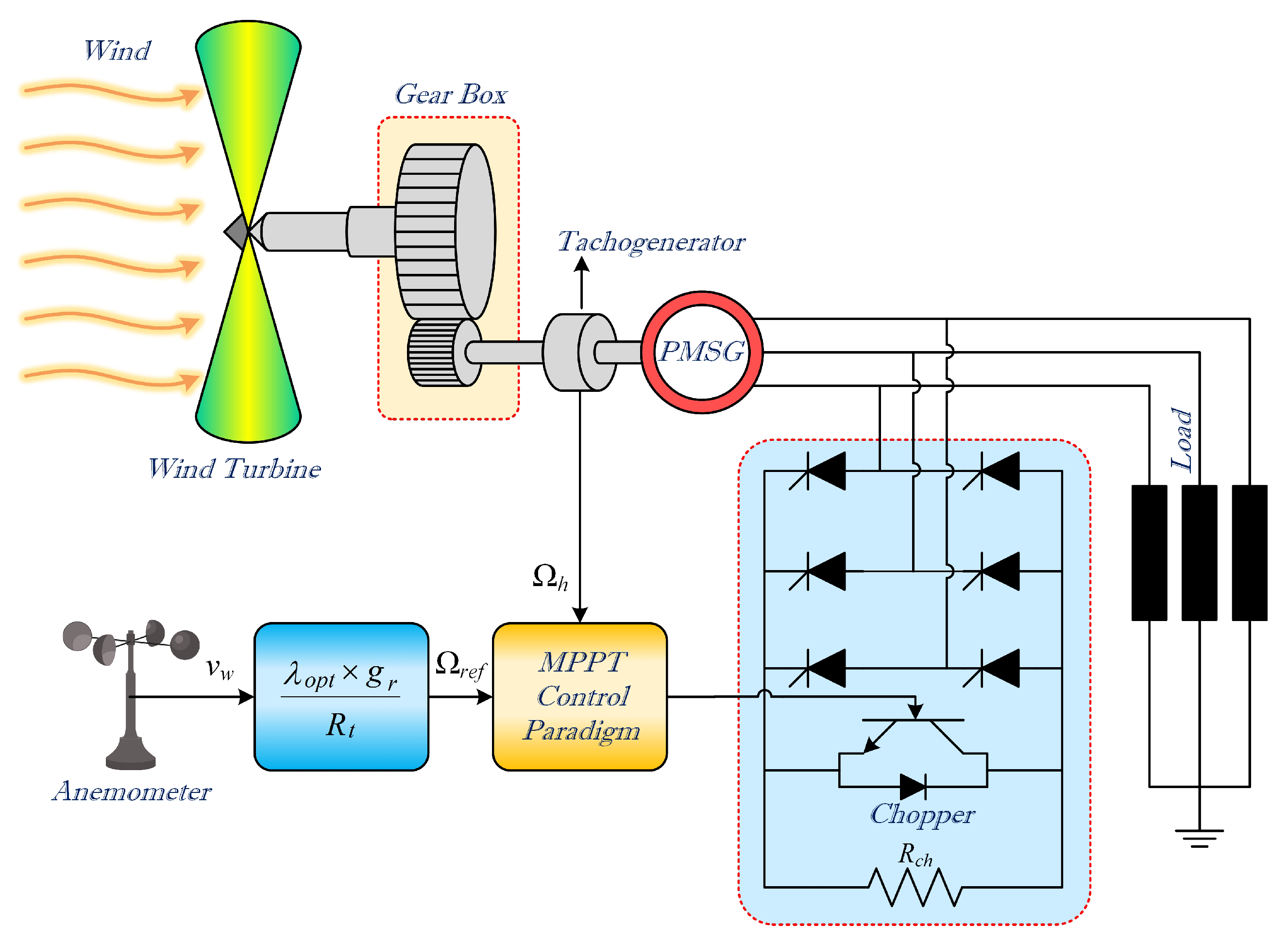
2. Mathematical Modeling of PMSG–WECS

This section covers the mathematical modeling of the standalone, fixed-pitch, variable speed PMSG–WECS. A schematic of the overall variable speed PMSG–WECS is demonstrated in Figure 1. The principal components of a typical variable speed PMSG–WECS include: a variable speed wind turbine (VSWT), a gearbox, power electronic converters and a PMSG coupled with a VSWT.

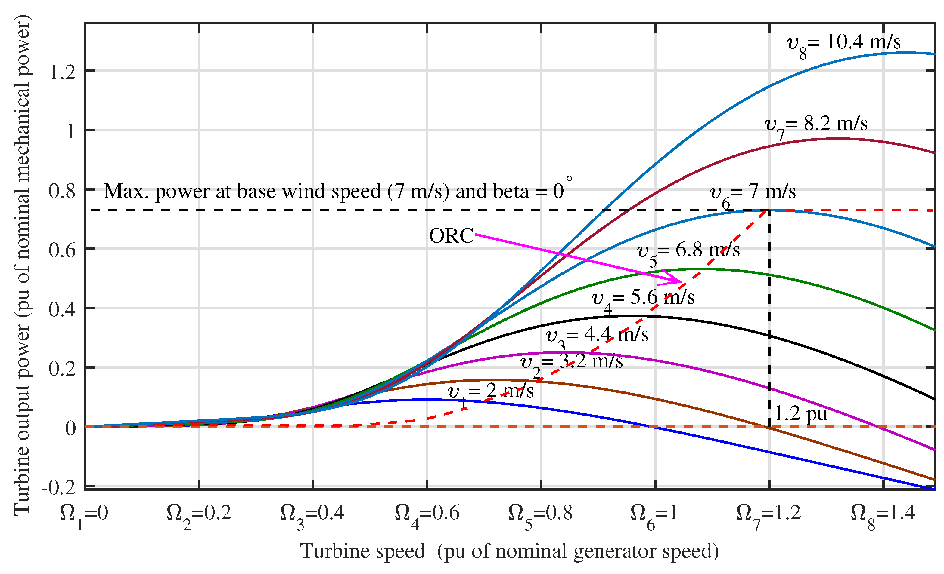
2.1. Wind Turbine Mathematical Modeling

The mechanical power, $P_m$, captured by the VSWT is expressed as follows [16]:

$$\begin{array}{c}\hfill P_m=\frac{1}{2}\rho \pi {R_t}^2{v}_w^3{C}_p(\lambda ,\beta )\end{array}$$

(1)

where $\rho$ denotes the air density (generally, its value is $1.25$ $\mathrm{kg}$/m${}^3$, at 10 ${}^{\circ }\mathrm{C}$, at sea level), $R_t$ stands for the turbine blade radius (m), $v_w$ represents the wind speed (m/s), and $C_p$ indicates the wind turbine rotor power conversion coefficient that defines the wind turbine rotor aerodynamic efficiency. Generally, $C_p$ varies with both the tip speed ratio, $\lambda$, and the blade pitch angle, $\beta$. However, $\beta$ is assumed to be a constant ($\beta =$ 0 ${}^{\circ }$) in this article.

$C_p$ is determined by numerical approximation; such as in [17], for $\beta =0^{\circ }$, it is given as follows:

$$\begin{array}{cc}\hfill & C_p\left(\lambda \right)=0.0061\lambda -0.0013{\lambda }^2+0.0081{\lambda }^3-9.7477\times {10}^{-4}{\lambda }^4-6.5416\times {10}^{-5}{\lambda }^5\hfill \\ & +1.3027\times {10}^{-6}{\lambda }^6-4.54\times {10}^{-7}{\lambda }^7\hfill \end{array}$$

(2)

$C_p$ has a unique maximum value (say, $C_{p_{max}}$) at a particular $\lambda$, called ${\lambda }_{opt}$. Thus, a VSWT tracks the $C_{p_{max}}$, while maintaining the tip speed ratio at its optimal value, ${\lambda }_{opt}$, for the maximum wind power extraction.

The ratio of the peripheral speed of the wind turbine blades to the wind speed indicates the tip speed ratio, as follows:

$$\begin{array}{c}\hfill \lambda =\frac{{\mathrm{\Omega }}_{\ell }{R}_t}{v_w}\end{array}$$

(3)

where ${\mathrm{\Omega }}_{\ell }$ represents the rotational speed of the wind turbine blades (rad/s, i.e., rotational speed of the low-speed shaft).

The wind turbine mechanical torque (aerodynamic torque), $T_m$, can be obtained from Equations (1) and (3), as follows:

$$\begin{array}{c}\hfill T_m=\frac{P_m}{{\mathrm{\Omega }}_{\ell }}=\frac{1}{2}\rho \pi R_t^3{v}_w^2{C}_t\left(\lambda \right)\end{array}$$

(4)

where $C_t\left(\lambda \right)=C_p\left(\lambda \right)/\lambda$ represents the wind turbine torque coefficient. It can be found from a second-order polynomial expression, as a function of the tip speed ratio, as follows:

$$\begin{array}{c}\hfill C_t\left(\lambda \right)={\alpha }_0+{\alpha }_1\lambda +{\alpha }_2{\lambda }^2\end{array}$$

(5)

Now, substituting Equations (3) and (5) into Equation (4), $T_m$ can also be expressed as follows:

$$\begin{array}{c}\hfill T_m=d_1{v}_w^2+\frac{d_2{v}_w{\mathrm{\Omega }}_h}{g_r}+\frac{d_3{\mathrm{\Omega }}_h^2}{g_r^2}\end{array}$$

(6)

where ${\mathrm{\Omega }}_h$ is rotational speed of the high speed shaft (PMSG rotor) and $g_r={\mathrm{\Omega }}_h/{\mathrm{\Omega }}_{\ell }$ is the gear ratio (or transmission ratio). Moreover,

$$\left\{\begin{array}{c}{d}_1=0.5\pi \rho R_t^3{\alpha }_0,d_2=0.5\pi \rho R_t^4{\alpha }_1,d_3=0.5\pi \rho R_t^5{\alpha }_2\hfill \\ {\alpha }_0=0.1253,{\alpha }_1=-0.0047,{\alpha }_2=-0.0005\hfill \end{array}\right.$$

Knowing $C_{p_{max}}$ and ${\lambda }_{opt}$, the optimal mechanical power, $P_{m_{opt}}$, generated by the VSWT can be worked out from Equation (1) by substituting Equation (3) into it as follows:

$$\begin{array}{c}\hfill P_{m_{opt}}=\frac{\rho \pi {R_t}^5{\mathrm{\Omega }}_{\ell }^3{C}_{p_{max}}\left(\lambda \right)}{2{\lambda }_{opt}^3}\end{array}$$

(7)

Figure 2 demonstrates the mechanical power output of the VSWT under different wind speeds. There exists a unique maximum power point, $P_{m_{opt}}$, at each wind speed. All these maximum power points constitute an optimal regime characteristic (ORC). The ORC indicates the operating region where the maximum possible energy can be extracted from the fluctuating wind. The primary goal of the MPPT control strategy is to continuously operate the VSWT on the ORC, despite fluctuations in the wind speed.

The optimal mechanical torque can be obtained from the optimal mechanical power given in Equation (7) as follows:

$$\begin{array}{c}\hfill T_{m_{opt}}=\frac{P_{m_{opt}}}{{\mathrm{\Omega }}_{\ell }}=\frac{\rho \pi R_t^5{\mathrm{\Omega }}_{\ell }^2{C}_{p_{max}}\left(\lambda \right)}{2{\lambda }_{opt}^3}\end{array}$$

(8)

Table 1. PMSG–WECS and the proposed maximum power point tracking (MPPT) controller parameters.

Name	Quantity	Value
Wind Turbine	Air density (at 10 ${}^{\circ }\mathrm{C}$, at sea level), $\rho$	$1.25$$\mathrm{kg}$/m${}^3$
	Turbine blade radius, $R_t$	$2.50$$\mathrm{m}$
	Transmission (or gear) ratio, $g_r$	7
	Average wind speed, $v_{w_{av}}$	7 $\mathrm{m}$/$\mathrm{s}$
	Optimal tip speed ratio, ${\lambda }_{opt}$	7
	Maximum power conversion coefficient, $C_{p_{max}}$	0.4762
PMSG	Stator resistance, $R_s$	3.30 $\mathrm{\Omega }$
	Stator d-axis inductance, $L_d$	$41.56$$\mathrm{mH}$
	Stator q-axis inductance, $L_q$	$41.56$$\mathrm{mH}$
	Magnetic flux, ${\mathrm{\Phi }}_m$	$438.20$$\mathrm{mWb}$
	Pole pairs, p	3
	High-speed shaft moment of inertia, $J_h$	$0.05522$$\mathrm{kg}$$\mathrm{m}$${}^2$
	Load inductance, $L_{ch}$	$0.008$$\mathrm{H}$
FDTSMC	Gain, $p_3$	3
	Gain, $q_3$	1
	Gain, $c_2$	100
	Gain, $c_3$	7000
	Gain, ${\beta }_3$	200
	Gain, ${\mathcal{K}}_1$	4000
	Gain, ${\mathcal{K}}_2$	0.1

and

Table 2. Specification of various important parameters.

Parameter	Value	Parameter	Value	Parameter	Value
$a_1$	0.1215	$b_3$	−6	$d_4$	2.6292
$a_2$	−27.1471	$b_4$	21.6288	${\xi }_1$	9.9399
$a_3$	−0.9486	$d_1$	3.8422	${\xi }_2$	−0.13316
$b_1$	0.1215	$d_2$	−0.3603	${\xi }_3$	$-5.059\times {10}^{-3}$
$b_2$	−27.1471	$d_3$	−0.0958	${\xi }_4$	2.6292

describe different significant parameters of the overall PMSG–WECS along with its control system.

2.2. Permanent Magnet Synchronous Generator Mathematical Modeling

The PMSG can be conveniently modeled in the d-q (or synchronously rotating) reference frame, where the zero components are discarded. The axis along the axis of the rotor is called the direct or the d-axis, while the axis perpendicular to the d-axis is known as the quadrature or q-axis.

For a standalone PMSG–WECS, the voltages on the d-q axes are considered as the output variables. Based on this concept, the PMSG model can be described in terms of the d-q axes voltages by the following group of equations [18,19]:

$$\begin{array}{c}\left(L_d+L_{ch}\right){\displaystyle \frac{d{i}_d}{dt}}=-\left(R_s+R_{ch}\right)i_d+p\left(L_q-L_{ch}\right)i_q{\mathrm{\Omega }}_h\hfill \\ \left(L_q+L_{ch}\right){\displaystyle \frac{d{i}_q}{dt}}=-\left(R_s+R_{ch}\right)i_q-p\left(L_d+L_{ch}\right)i_q{\mathrm{\Omega }}_h+p{\mathrm{\Phi }}_m{\mathrm{\Omega }}_h\hfill \\ {\displaystyle J_h\frac{d{\mathrm{\Omega }}_h}{dt}=\frac{T_m}{g_r}-T_{em}=\frac{T_m}{g_r}-\left[p\left(L_d-L_q\right)i_d{i}_q+p{\mathrm{\Phi }}_m{i}_q\right]=\frac{d_1{v}_w^2}{g_r}+\frac{d_2{v}_w{\mathrm{\Omega }}_h}{g_r^2}}\hfill \\ {\displaystyle +\frac{d_3{\mathrm{\Omega }}_h^2}{g_r^3}-p{\mathrm{\Phi }}_m{i}_q}\hfill \end{array}\}$$

(9)

where $R_s$ denotes the stator resistance, $L_d$ and $L_q$ represent the stator d- and q-$axis$ inductances, respectively, $i_d$ and $i_q$ stand for the d- and q-$axis$ stator currents, respectively, p indicates the number of pole pairs, ${\mathrm{\Phi }}_m$ indicates the maximum value of magnetic flux and $T_{em}$ represents the electromagnetic torque of the PMSG, resulting from the interaction between the stator and rotor fluxes. Moreover, $J_h$ denotes the moment of inertia of the high-speed shaft (PMSG) and $R_{ch}$, $L_{ch}$ indicate the resistance and inductance of the load, respectively. In Equation (9), the non-salient pole type of PMSG has been considered, for which $L_d=L_q$.

The WECS is inherently a highly nonlinear system. The objective of this work is to maximize the power extraction from the PMSG–WECS, which is accomplished by controlling the shaft speed. For this purpose, the nonlinear PMSG–WECS model can be written in state-space representation as follows:

$$\left\{\begin{array}{c}\dot{\mathbf{x}}=f\left(\mathbf{x}\right)+g\left(\mathbf{x}\right)u\hfill \\ y=h\left(\mathbf{x}\right)\hfill \end{array}\right.$$

where

$$\begin{array}{c}\underset{\dot{\mathbf{x}}}{\underbrace{\left[\begin{array}{c}{\displaystyle {\dot{x}}_1}\\ \\ {\displaystyle {\dot{x}}_2}\\ \\ {\displaystyle {\dot{x}}_3}\end{array}\right]}}=\underset{f\left(\mathbf{x}\right)}{\underbrace{\left[\begin{array}{c}{a}_2{x}_1+a_3{x}_2{x}_3\\ \\ b_2{x}_2+b_3{x}_1{x}_3+b_4{x}_3\\ \\ {\displaystyle \frac{1}{J_h}\left(\frac{d_1{v}_w^2}{g_r}+\frac{d_2{v}_w{x}_3}{g_r^2}+\frac{d_3{x}_3^2}{g_r^3}-p{\mathrm{\Phi }}_m{x}_2\right)}\end{array}\right]}}+\underset{g\left(\mathbf{x}\right)}{\underbrace{\left[\begin{array}{c}{\displaystyle -\frac{x_1}{a_1}}\\ \\ {\displaystyle -\frac{x_2}{b_1}}\\ \\ 0\end{array}\right]}}.\underset{u}{\underbrace{R_{ch}}}\hfill \\ y=\underset{h\left(\mathbf{x}\right)}{\underbrace{{\mathrm{\Omega }}_h}}\hfill \end{array}\}$$

(10)

where $f\left(\mathbf{x}\right)={\left[f_1{f}_2{f}_3\right]}^T$, $g\left(\mathbf{x}\right)={\left[g_1{g}_2{g}_3\right]}^T$, $\mathbf{x}={\left[x_1{x}_2{x}_3\right]}^T={\left[i_d{i}_q{\mathrm{\Omega }}_h\right]}^T\in {\mathbb{R}}^n$ represents the state vector, $f\left(\mathbf{x}\right)$ and $g\left(\mathbf{x}\right)$ stand for the nonlinear smooth vector fields, and u and y indicate the control input and output, respectively. Moreover,

$$\left\{\begin{array}{c}{\displaystyle a_1=L_d+L_{ch};a_2=-\frac{R_s}{a_1};a_3=\frac{p(L_q-L_{ch})}{a_1}}\hfill \\ \\ {\displaystyle b_1=L_q+L_{ch};b_2=-\frac{R_s}{b_1};b_3=-\frac{p(L_d+L_{ch})}{b_1};b_4=\frac{p{\mathrm{\Phi }}_m}{b_1}}\hfill \end{array}\right.$$

Table 1 and Table 2 describe different significant parameters of the overall PMSG–WECS along with its control system.

3. Coordinates Transformation

To express the system in normal form, the coordinates transformation must be carried out, as follows:

$$\begin{array}{c}{\displaystyle z_1=h\left(\mathbf{x}\right)=x_3={\mathrm{\Omega }}_h}\hfill \\ {\displaystyle z_2=L_{f}h\left(\mathbf{x}\right)=\frac{\partial h\left(\mathbf{x}\right)}{\partial x}f\left(\mathbf{x}\right)={\xi }_1{v}_w^2+{\xi }_2{v}_w{x}_3+{\xi }_3{x}_3^2-{\xi }_4{x}_2}\hfill \\ {\displaystyle z_3=a_3\frac{x_1}{x_2}}\hfill \end{array}\}$$

(11)

where ${\displaystyle {\xi }_1=\frac{d_1}{J_h{g}_r}}$, ${\displaystyle {\xi }_2=\frac{d_2}{J_h{g}_r^2}}$, ${\displaystyle {\xi }_3=\frac{d_3}{J_h{g}_r^3}}$ and ${\displaystyle {\xi }_4=d_4=p{\mathrm{\Phi }}_m}$.

Since, the system under consideration possesses a relative degree, $r<n$ (system order), where $r=2$ and $n=3$, it implies that the system is only partially linearizable [20,21]. Moreover, the input-output form (normal form) can be expressed as follows:

$$\begin{array}{c}{\displaystyle {\dot{z}}_1=z_2}\hfill \\ {\displaystyle {\dot{z}}_2=L_f^{2}h\left(\mathbf{x}\right)+L_g{L}_{f}h\left(\mathbf{x}\right)u}\hfill \\ {\dot{z}}_3=L_f^{3}h\left(\mathbf{x}\right)+L_g{L}_f^{2}h\left(\mathbf{x}\right)\dot{u}\hfill \end{array}\}$$

(12)

where one of the transformed system states, i.e., $z_3$ represents the internal (or zero) dynamic state. Now, the Lie derivatives are given as follows:

$$\begin{array}{c}{L}_f^{2}h\left(\mathbf{x}\right)=-d_4(b_2{x}_1+b_3{x}_1{x}_3+b_4{x}_3)+(d_2{v}_w+2d_3{x}_3)({\xi }_1{v}_w^2+{\xi }_2{v}_w{x}_3+{\xi }_3{x}_3^2-{\xi }_4{x}_2)\hfill \\ {\displaystyle L_g{L}_{f}h\left(\mathbf{x}\right)=-\frac{d_4{x}_2}{a_1}\ne 0}\hfill \end{array}\}$$

(13)

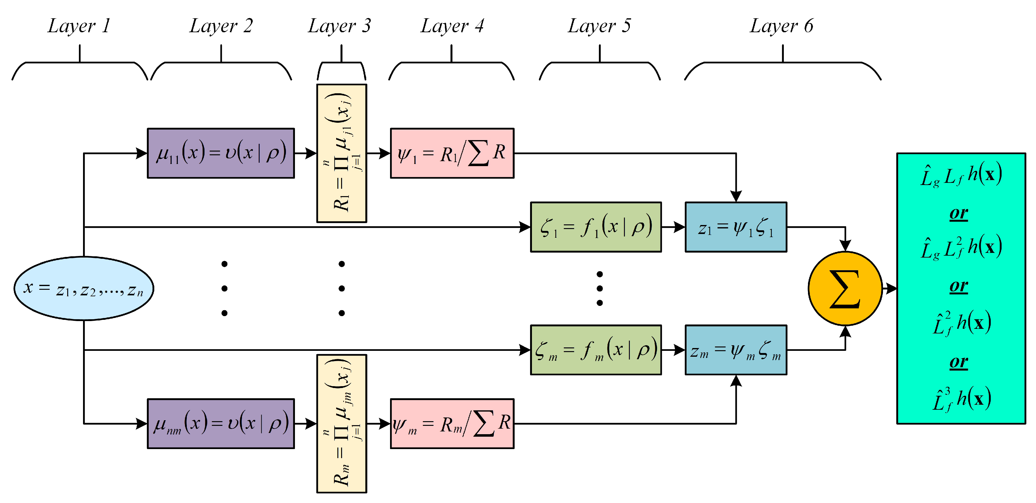
4. Lie Derivatives Estimation via Adaptive Neuro-Fuzzy Inference System

In practical contexts, one may not be available with the nonlinear terms and aerodynamic forces. Hence, in this work, an offline Takagi–Sugeno–Kang (TSK)-based ANFIS scheme is designed for the estimation of the nonlinear drift of the PMSG–WECS (i.e., $L_g{L}_{f}h\left(\mathbf{x}\right)$, $L_g{L}_f^{2}h\left(\mathbf{x}\right)$, $L_f^{2}h\left(\mathbf{x}\right)$ and $L_f^{3}h\left(\mathbf{x}\right)$). The TSK-based ANFIS is a MISO (multiple-input-single-output) system [22]. Four ANFIS networks are trained for estimating the system Lie derivatives using the inputs ($z_1$, $z_2$, $z_3$ and $v_w$) and outputs ($L_g{L}_{f}h\left(\mathbf{x}\right)$, $L_g{L}_f^{2}h\left(\mathbf{x}\right)$, $L_f^{2}h\left(\mathbf{x}\right)$ and $L_f^{3}h\left(\mathbf{x}\right)$). The input-output data are generated by simulating the system for a particular wind speed profile. The ANFIS network then mimics the relationships between the inputs and the corresponding outputs. The ANFIS estimation network comprises six layers. Layer 1 consists of all the inputs that are available during the estimation process. Layer 2 generates the membership functions based on triangular functions. Layer 3 represents the antecedent connective part of the extracted IF-THEN fuzzy rule. Layers 4, 5 and 6 represent the normalization layer, the consequent or regressor layer and the summation layer, respectively.

The complete ANFIS network structure for Lie derivatives estimation is demonstrated in Figure 3.

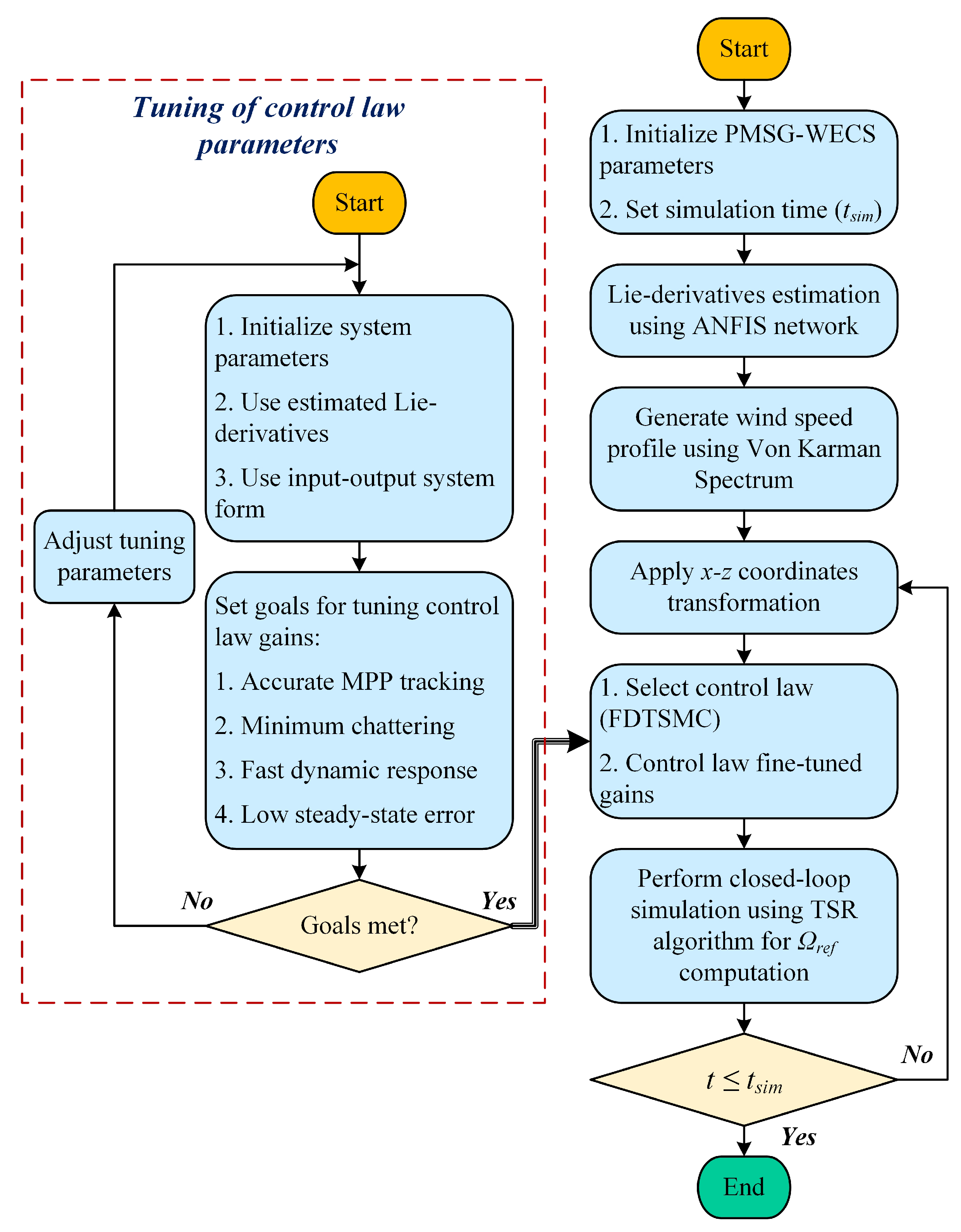
5. MPPT Control Design for PMSG–WECS

The main goal of the MPPT control design is to maximize the power output of the PMSG–WECS. This goal is accomplished by proposing an FDTSMC-based MPPT control strategy.

The conventional TSMC strategy may not be able to guarantee the same convergence speed for the system states located distant from the equilibrium point, O. However, it can offer a finite-time convergence for the system states located near the equilibrium point.

The conventional TSMC concept was first introduced in [23], for which the nonlinear sliding surface can be expressed as follows:

$$s_1=\dot{e}+{\beta }_1{e}^{\frac{q_1}{p_1}}=0$$

(14)

where e represents the tracking error and ${\beta }_1$, $p_1$, $q_1>0$. Note that both $p_1$ and $q_1$ must be odd integers, such that $\left(p_1>q_1\right)$. It can easily be verified that for any given initial tracking error, $e\left(0\right)\ne 0$, the dynamics expressed in Equation (14) will converge to $e=0$ in a finite time, as determined by the reaching time, $t^{s_1}=[p_1/\left\{{\beta }_1\left(p_1-q_1\right)\right\}]{\left|e\left(0\right)\right|}^{\left(p_1-q_1\right)/p_1}$, obtained from the analytical solution of Equation (14). The equilibrium point O is termed as the terminal attractor. The reaching time can be tuned by proper selection of the parameters ${\beta }_1$, $p_1$ and $q_1$.

The inclusion of the nonlinear term $e^{q_1/p_1}$ in Equation (14) improves the convergence towards the equilibrium point such that the closer the $e^{q_1/p_1}$ is to the equilibrium point, the faster the convergence will be, thus offering a finite-time convergence. However, for the system states located distant from the equilibrium point, the conventional TSMC strategy does not outperform its conventional SMC counterpart (where $p_1=q_1$) because the $e^{q_1/p_1}$ term now tends to retard the convergence towards the equilibrium point. To counteract this problem, a solution has been proposed in [24] that is known as the FTSMC, for which the nonlinear sliding surface can be expressed as follows:

$$s_2=\dot{e}+c_{1}e+{\beta }_2{e}^{q_2/p_2}=0$$

(15)

where $c_1$, ${\beta }_2$, $p_2$, $q_2>0$. Note that both $p_2$ and $q_2$ must be odd integers, such that $\left(p_2>q_2\right)$. Thus, Equation (15) gives $\dot{e}=-c_{1}e-{\beta }_2{e}^{q_2/p_2}$. By properly choosing $p_2$ and $q_2$, for a given initial tracking error $e\left(0\right)\ne 0$, the dynamics expressed in Equation (15) will converge to $e=0$ in a finite time. Physically, it can be interpreted as: when e is located far away from the equilibrium point, the approximate dynamics can then be expressed as: $\dot{e}=-c_{1}e$, which offers a fast and finite-time convergence. However, when e is located close to the equilibrium point, the approximate dynamics then become: $e=-{\beta }_2{e}^{q_2/p_2}$, which is the terminal attractor offering fast and finite-time convergence. More precisely, the analytical solution of Equation (15) gives the exact time to reach the equilibrium point (reaching time) as follows:

$$t^{s_2}=\frac{p_2}{c_1\left(p_2-q_2\right)}\left[ln\{c_{1}e{\left(0\right)}^{\left(p_2-q_2\right)/p_2}+{\beta }_2\}-ln{\beta }_2\right]$$

(16)

FDTSMC-Based MPPT Control Design for PMSG–WECS

The FTSMC renders the advantages of fast dynamic response, high steady-state tracking accuracy and finite-time convergence. However, chattering of the control signal due to the switching action of the discontinuous control signal, and sensitivity to high-frequency noise, still remain as the main disadvantages of the FTSMC. To counteract these issues, a novel strategy has been proposed in [25], namely the global FDTSMC. In the stated strategy, the time derivative of the control input has been taken as the control variable for the augmented system such that the control input appears as chattering-free due to an integrator (acting as a low-pass filter) placed next to the system.

In this article, the FDTSMC offers a finite-time rotor speed tracking error convergence of the PMSG–WECS for ensuring the MPPT. This control strategy is developed using a function augmented nonlinear sliding surface that guarantees the tracking error convergence to the equilibrium point in a finite time. Moreover, the high-frequency chattering is completely eliminated by eliminating the reaching phase.

The input-output form for FDTSMC can be described as follows:

$$\begin{array}{c}{\dot{z}}_1=z_2\hfill \\ {\dot{z}}_2={\widehat{L}}_f^{2}h\left(\mathbf{x}\right)+{\widehat{L}}_g{L}_{f}h\left(\mathbf{x}\right)u\hfill \\ {\dot{z}}_3={\widehat{L}}_f^{3}h\left(\mathbf{x}\right)+{\widehat{L}}_g{L}_f^{2}h\left(\mathbf{x}\right)\dot{u}\hfill \end{array}\}$$

(17)

where ${\widehat{L}}_f^{3}h\left(\mathbf{x}\right)$ and ${\widehat{L}}_g{L}_f^{2}h\left(\mathbf{x}\right)$ have been expressed in Equations (A1) and (A2), in Appendix A, respectively.

The nonlinear sliding surface for the proposed FDTSMC can be expressed as follows:

$$s_3=\dot{\sigma }+c_2\sigma +{\beta }_3{\sigma }^{q_3/p_3}$$

(18)

where $c_2$, ${\beta }_3$, $p_3$, $q_3>0$. Note that both $p_3$ and $q_3$ must be odd integers, such that ($p_3>q_3$). The term $\sigma$ in Equation (18) denotes a sliding mode surface that can be expressed as follows:

$$\sigma =\dot{e}+c_{3}e=(z_2-{\dot{z}}_{ref})+c_3(z_1-z_{ref})$$

(19)

Now, the successive differentiation of Equation (19) yields:

$$\begin{array}{c}\dot{\sigma }=({\dot{z}}_2-{\ddot{z}}_{ref})+c_3({\dot{z}}_1-{\dot{z}}_{ref})=(z_3-{\ddot{z}}_{ref})+c_3(z_2-{\dot{z}}_{ref})\hfill \\ \hfill \ddot{\sigma }=({\dot{z}}_3-{\stackrel{⃛}{z}}_{ref})+c_3({\dot{z}}_2-{\ddot{z}}_{ref})={\widehat{L}}_f^{3}h\left(\mathbf{x}\right)+{\widehat{L}}_g{L}_f^{2}h\left(\mathbf{x}\right)\dot{u}-{\stackrel{⃛}{z}}_{ref}+c_3\left(\ddot{e}\right)\end{array}\}$$

(20)

Next, the FDTSMC sliding surface expressed in Equation (18) is differentiated and simplified using Equation (20) in order to derive the equivalent controller as follows:

$$\dot{s_3}={\widehat{L}}_f^{3}h\left(\mathbf{x}\right)+{\widehat{L}}_g{L}_f^{2}h\left(\mathbf{x}\right)\dot{u}-{\stackrel{⃛}{z}}_{ref}+c_3\ddot{e}+c_2\dot{\sigma }+{\beta }_3\frac{q_3}{p_3}{\sigma }^{\left(\frac{q_3}{p_3}-1\right)}\dot{\sigma }$$

(21)

The equivalent controller, ${\dot{u}}_{eqD}$, can be obtained by setting Equation (21) to zero as follows:

$${\dot{u}}_{eqD}=\frac{-1}{{\widehat{L}}_g{L}_f^{2}h\left(\mathbf{x}\right)}\left[{\widehat{L}}_f^{3}h\left(\mathbf{x}\right)-{\stackrel{⃛}{z}}_{ref}+c_3\ddot{e}+c_2\dot{\sigma }+{\beta }_3\frac{q_3}{p_3}{\sigma }^{\left(\frac{q_3}{p_3}-1\right)}\dot{\sigma }\right]$$

(22)

While, the discontinuous controller, ${\dot{u}}_{discD}$, can be given as follows:

$${\dot{u}}_{discD}=-{\mathcal{K}}_1{s}_3-{\mathcal{K}}_{2}sign\left(s_3\right)$$

(23)

where ${\mathcal{K}}_1$, ${\mathcal{K}}_2>0$ are the switching controller gains.

Finally, the FDTSMC-based MPPT law is obtained by combining Equations (22) and (23), and passing through an integrator (low-pass filter) as follows:

$$\begin{array}{cc}\hfill & u_{FDTSMC}=\int [\underset{{\dot{u}}_{eqD}}{\underbrace{\frac{-1}{{\widehat{L}}_g{L}_f^{2}h\left(\mathbf{x}\right)}\left\{{\widehat{L}}_f^{3}h\left(\mathbf{x}\right)-{\stackrel{⃛}{z}}_{ref}+c_3\ddot{e}+c_2\dot{\sigma }+{\beta }_3\frac{q_3}{p_3}{\sigma }^{\left(\frac{q_3}{p_3}-1\right)}\dot{\sigma }\right\}}}\hfill \\ & \underset{{\dot{u}}_{discD}}{\underbrace{-{\mathcal{K}}_1{s}_3-{\mathcal{K}}_{2}sign\left(s_3\right)}}].dt\hfill \end{array}$$

(24)

The computational flow chart for implementation of the proposed MPPT strategy is depicted in Figure 4, while the closed-loop control system for PMSG–WECS is given in Figure 5.

6. Stability Analysis

To verify the PMSG–WECS closed-loop system stability under FDTSMC, Lyapunov theory is employed.

Stability Analysis for FDTSMC

First of all, a Lyapunov candidate function, $V_{f_1}$, and its derivative, ${\dot{V}}_{f_1}$, are defined along the system trajectory as follows:

$$\begin{array}{c}{V}_{f_1}=\frac{1}{2}{s}_3^2\hfill \\ {\dot{V}}_{f_1}=s_3{\dot{s}}_3\hfill \end{array}\}$$

(25)

Now, ${\dot{s}}_3$ from Equation (21) is substituted into Equation (25) as follows:

$${\dot{V}}_{f_1}=s_3\left[{\widehat{L}}_f^{3}h\left(\mathbf{x}\right)+{\widehat{L}}_g{L}_f^{2}h\left(\mathbf{x}\right){\dot{u}}_{FDTSMC}-{\stackrel{⃛}{z}}_{ref}+c_3\ddot{e}+c_2\dot{\sigma }+{\beta }_3\frac{q_3}{p_3}{\sigma }^{\left(\frac{q_3}{p_3}-1\right)}\dot{\sigma }\right]$$

(26)

Now, $u_{FDTSMC}$ from Equation (24) is substituted into Equation (26), giving:

$${\dot{V}}_{f_1}=-{\mathcal{K}}_1{s}_3^2-{\mathcal{K}}_2{s}_{3}sign\left(s_3\right)\le -{\mathcal{K}}_1{s}_3^2-{\mathcal{K}}_2\left|s_3\right|\therefore \forall {\mathcal{K}}_1,{\mathcal{K}}_2>0,{\dot{V}}_{f_1}<0$$

(27)

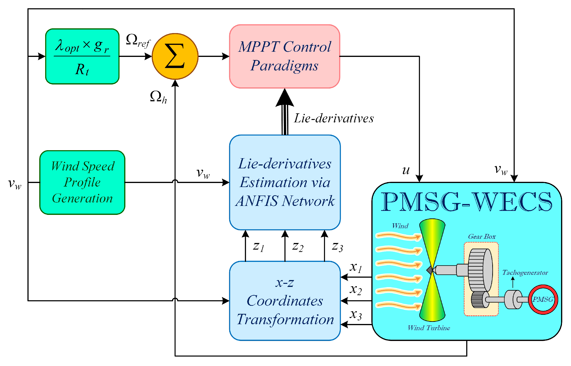
7. Simulation Results and Discussion

In this section, the proposed nonlinear MPPT control scheme, namely FDTSMC, is tested and evaluated in MATLAB/Simulink through simulations. The FTSMC [26], CSMC, FBLC [27] and PID have been used as benchmarks to manifest the superior tracking performance of the proposed MPPT paradigm. For performance evaluation, the wind speed is assumed to have a stochastic profile.

Figure 4 and Figure 5 demonstrate the application of the proposed nonlinear MPPT control paradigm to the standalone, variable speed, fixed-pitch, 3 $\mathrm{k}$$\mathrm{W}$ PMSG–WECS. The MPPT strategy ensures the maximum power extraction from the VSWT while keeping the tip speed ratio, $\lambda$, at its optimal value, ${\lambda }_{opt}$. Table 1 describes different significant parameters of the proposed FDTSMC.

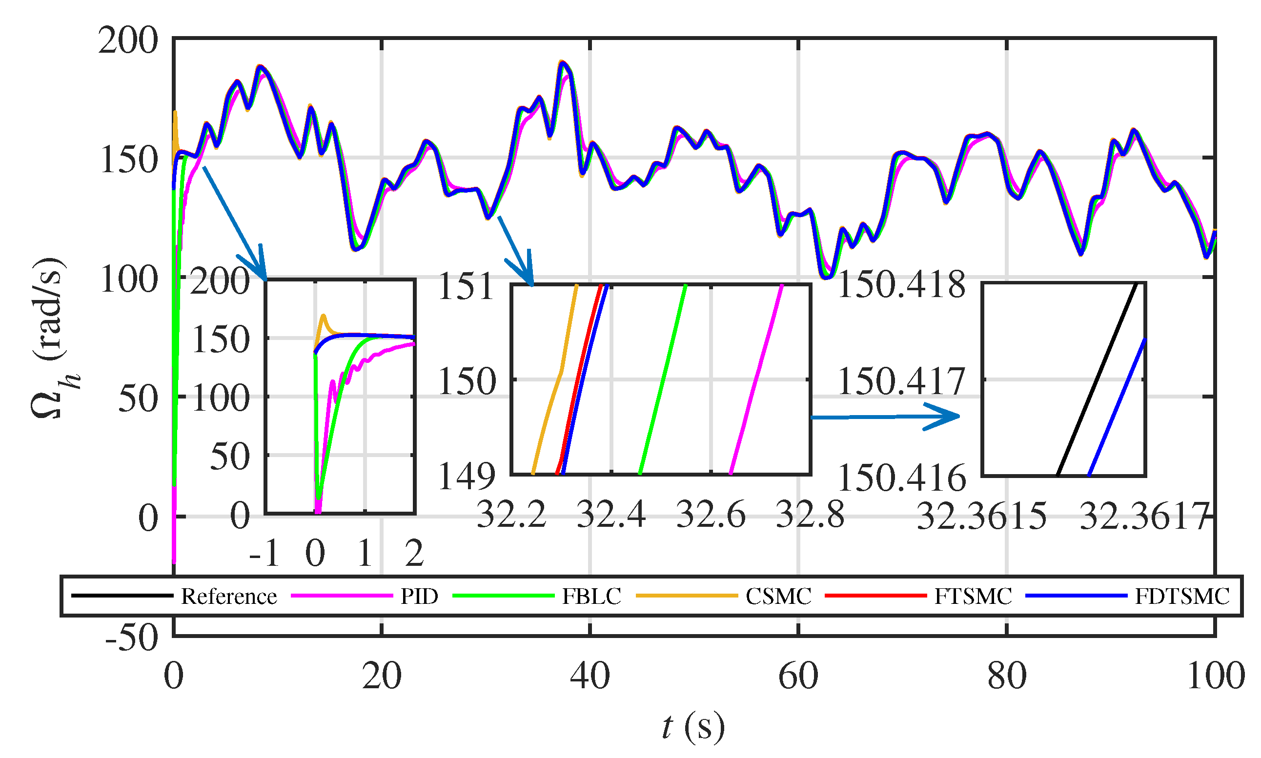
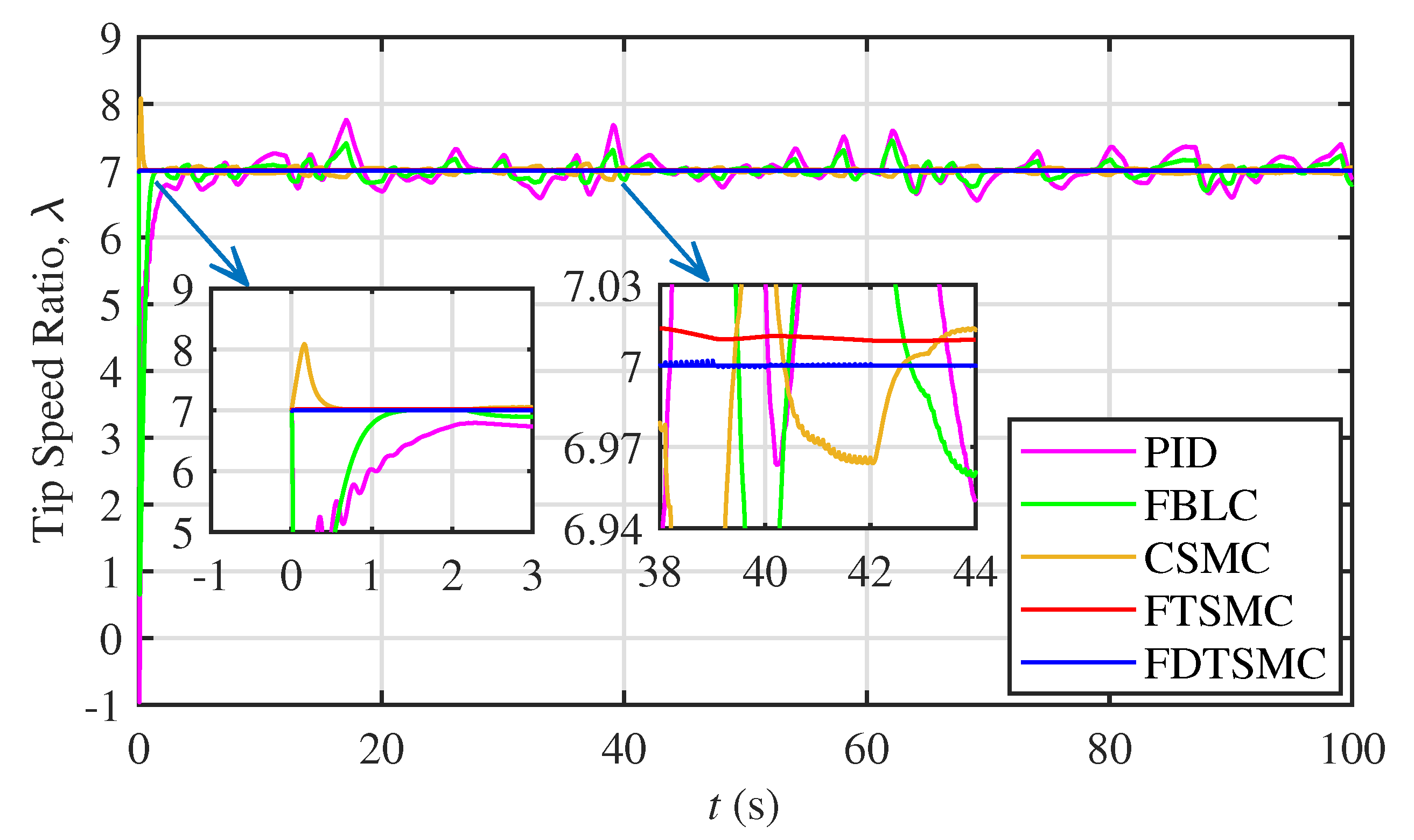
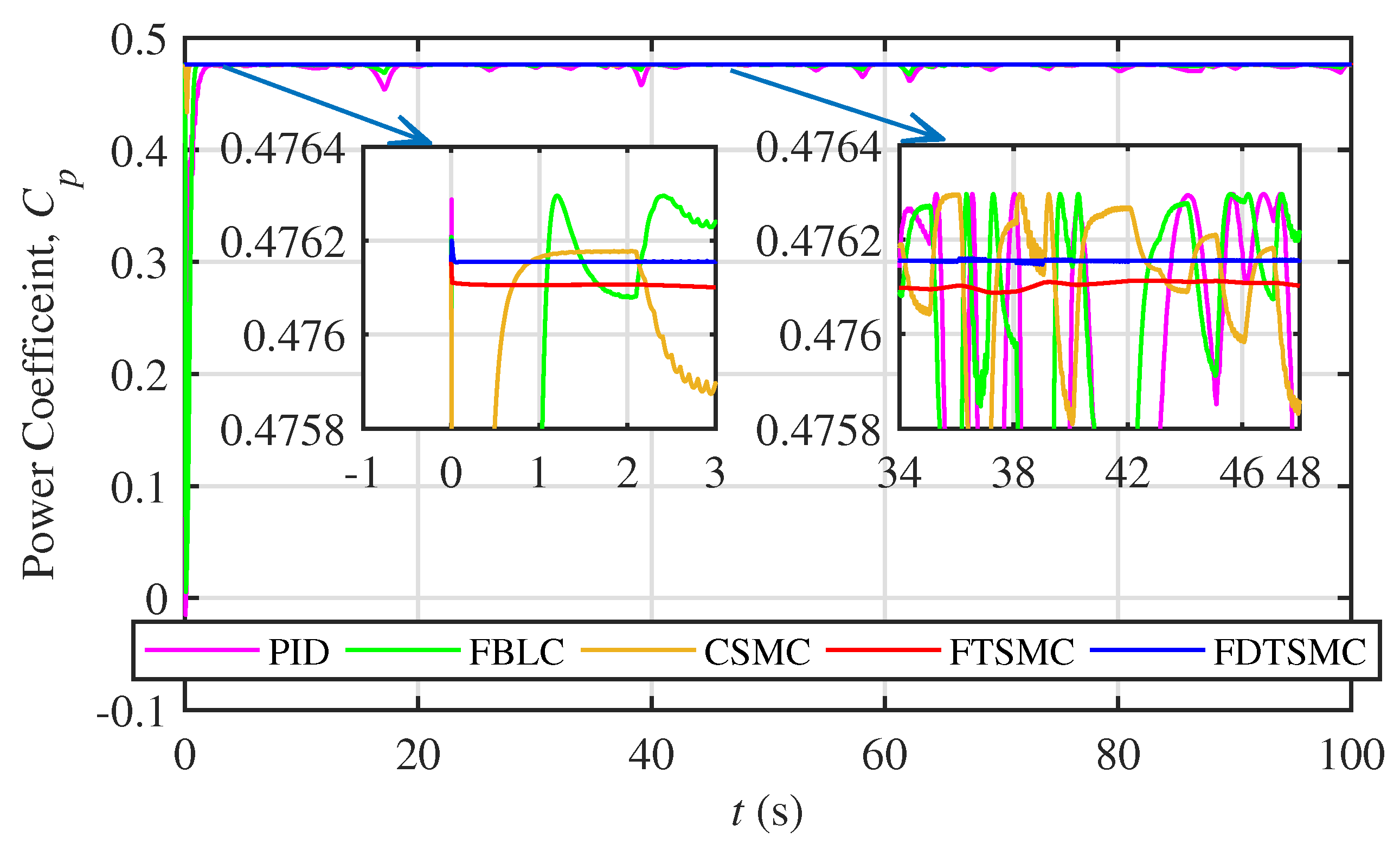
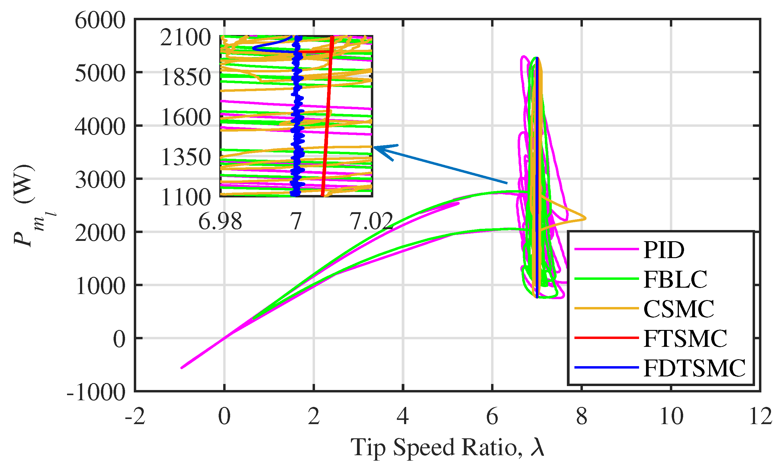
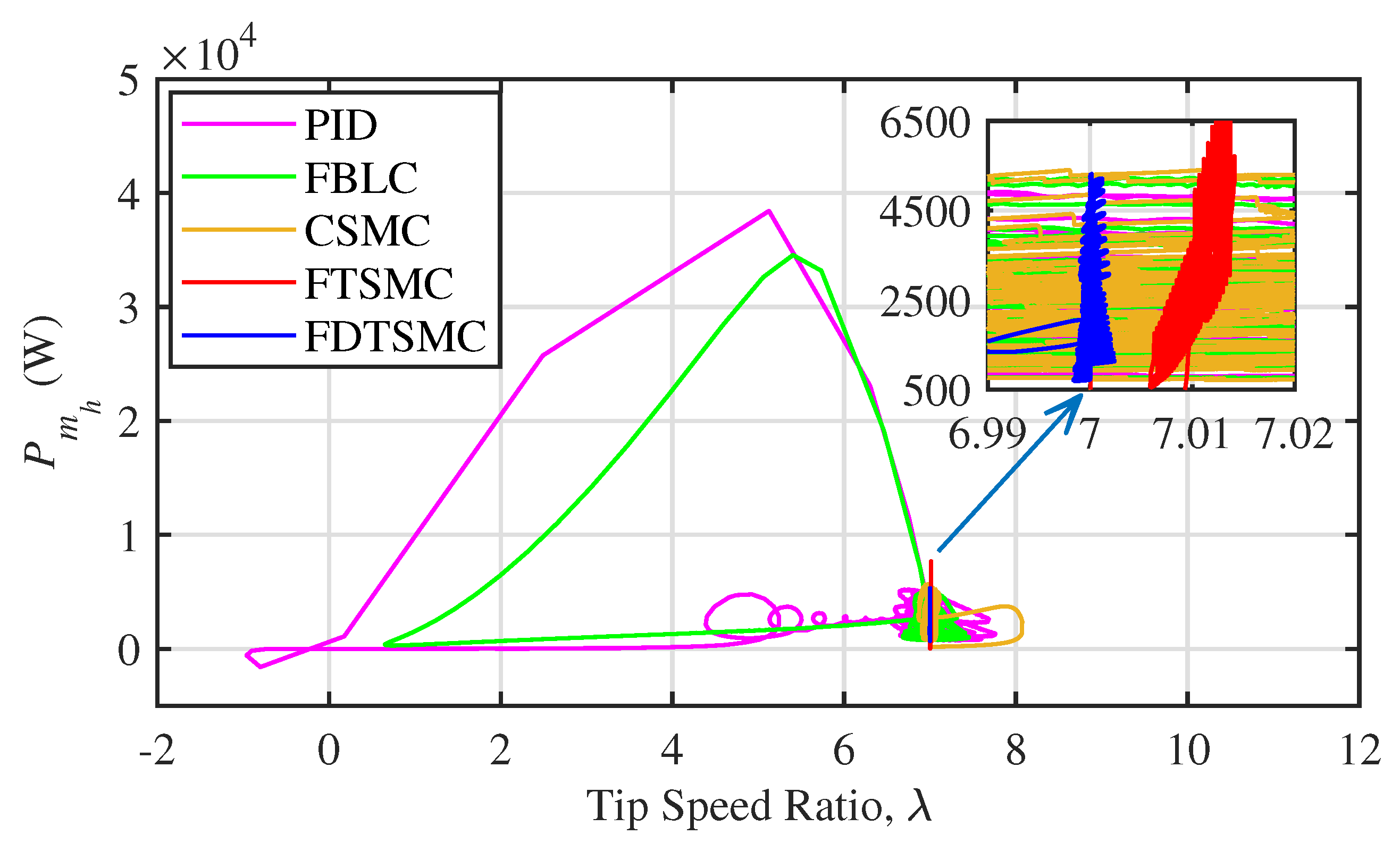
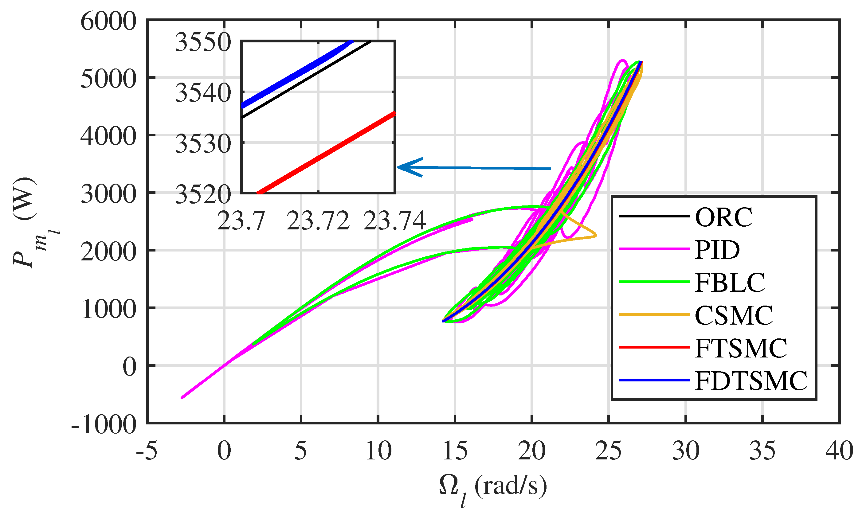
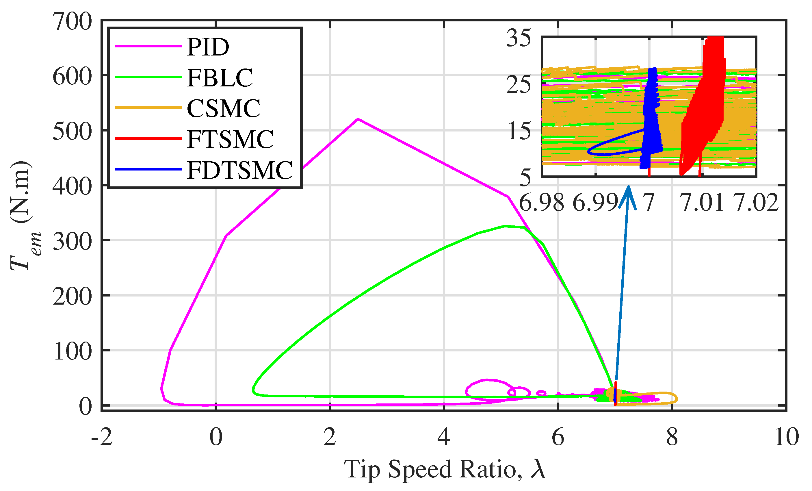
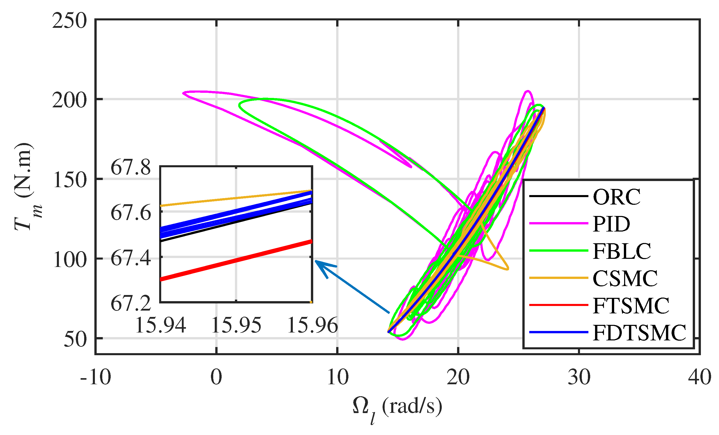
7.1. Performance Evaluation under Stochastic Wind Speed Profile

The performance of the proposed MPPT paradigm has been tested and evaluated, in this section, for a 3 $\mathrm{k}$$\mathrm{W}$ PMSG–WECS under a stochastic wind speed profile that comprises rapid and frequent wind speed fluctuations. The maximum power conversion coefficient, $C_{p_{max}}=0.4762$, computed from Equation (2) occurs at an optimal tip speed ratio, ${\lambda }_{opt}=7$. The simulations are performed for a 100 $\mathrm{s}$ horizon at an average wind speed of, $v_{w_{av}}=7$ $\mathrm{m}$/$\mathrm{s}$ (also depicted in Figure 2).

Figure 6 demonstrates the PMSG rotational speed tracking performance. It is evident from the zoomed-in segments of the figure that the FDTSMC is offering a superior tracking performance among its competitors. Moreover, both the FTSMC and FDTSMC offer a finite-time convergence. The superior performance of the FDTSMC to the FTSMC, CSMC, FBLC and PID, as well as the finite-time convergence of both the FTSMC and FDTSMC, are also evident from the speed tracking error of the PMSG, as depicted in Figure 7. The CSMC exhibits slightly better performance than both the FBLC and PID.

Figure 8 indicates the tip speed ratio performance of the VSWT. The PID has the worst performance, and it offers a lot of oscillations around the ${\lambda }_{opt}$. However, both the FTSMC and FDTSMC are accurately tracking the ${\lambda }_{opt}$ with FDTSMC being the best MPPT candidate.

Figure 9 shows the power conversion coefficient of the VSWT. It is clear that both the FTSMC and FDTSMC strategies are tracking the optimal power conversion coefficient, $C_{p_{max}}=0.4762$, throughout the selected stochastic wind speed profile, thus guaranteeing the maximum wind power extraction. The zoomed-in segments of the figure clearly depict that, based on the $C_{p_{max}}$ tracking, the FDTSMC is the best MPPT candidate, while the PID is the worst.

Figure 10 and Figure 11 indicate the low-speed shaft mechanical power and the high-speed shaft mechanical power versus the tip speed ratio, respectively. It is evident that both the FTSMC and the FDTSMC strategies maintain the low-speed as well as the high-speed shaft mechanical powers in the close neighborhood of the optimal tip speed ratio, ${\lambda }_{opt}$. On the other hand, both the FBLC and PID techniques have very poor performance on account of having a lot of power fluctuations around the optimal tip speed ratio.

Figure 12 represents the low-speed shaft mechanical power versus the low-speed shaft rotational speed. The proposed MPPT controller efficiently maintains the rotational speed of the VSWT in such a manner that the system operates on the ORC (optimal regimes characteristic)—that is, the region where the maximum wind power can be extracted. However, both the FBLC and PID schemes experience a lot of speed as well as mechanical power fluctuations.

Figure 13 illustrates the PMSG electromagnetic torque versus the tip speed ratio. Since both the FTSMC- and the FDTSMC-based MPPT candidates maintain the torque at the optimal tip speed ratio, ${\lambda }_{opt}=7$, it implies that both are capable of extracting the maximum wind power. The FDTSMC has the best, while the PID has the worst performance because of frequent torque fluctuations. Similarly, Figure 14 shows the VSWT mechanical torque versus the low-speed shaft rotational speed. Again, both the FTSMC- and the FDTSMC-based MPPT candidates maintain the torque around the ORC. It signifies that these two MPPT strategies are capable of extracting the maximum wind power, with FDTSMC being superior to the remaining MPPT candidates.

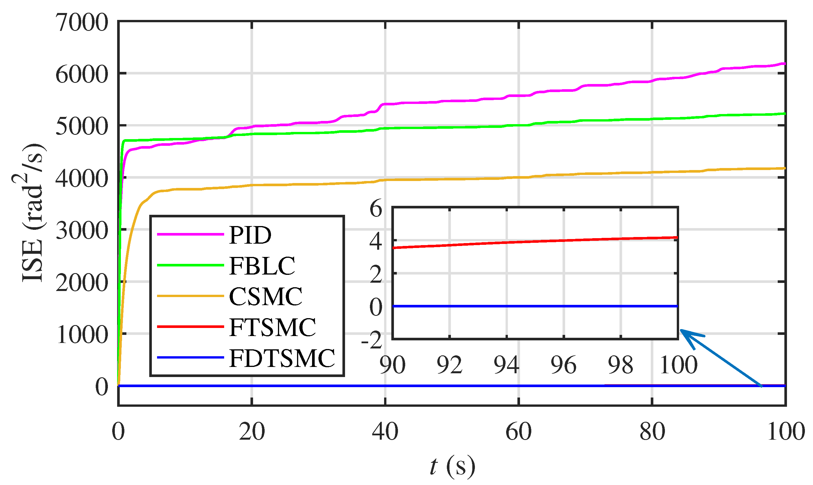
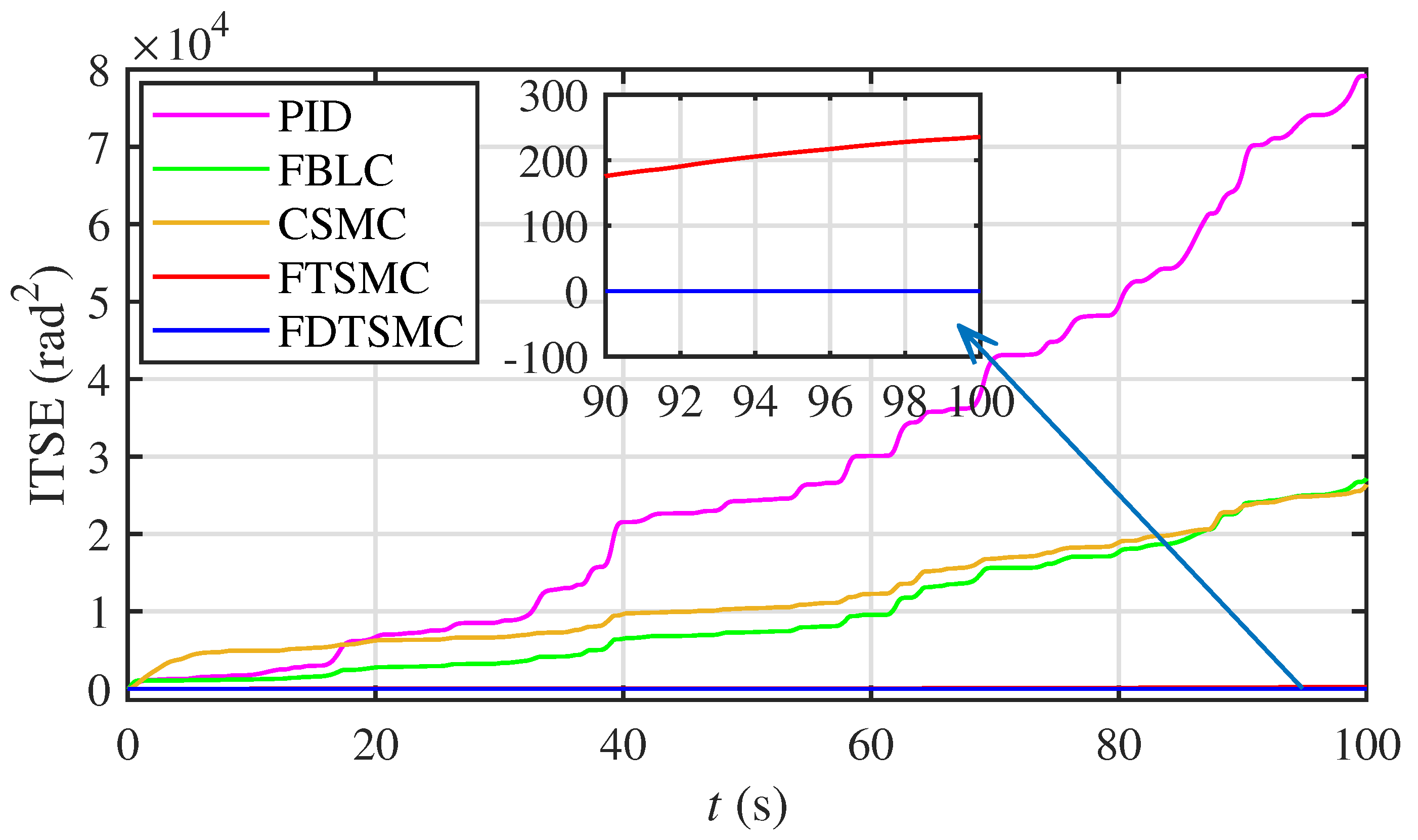
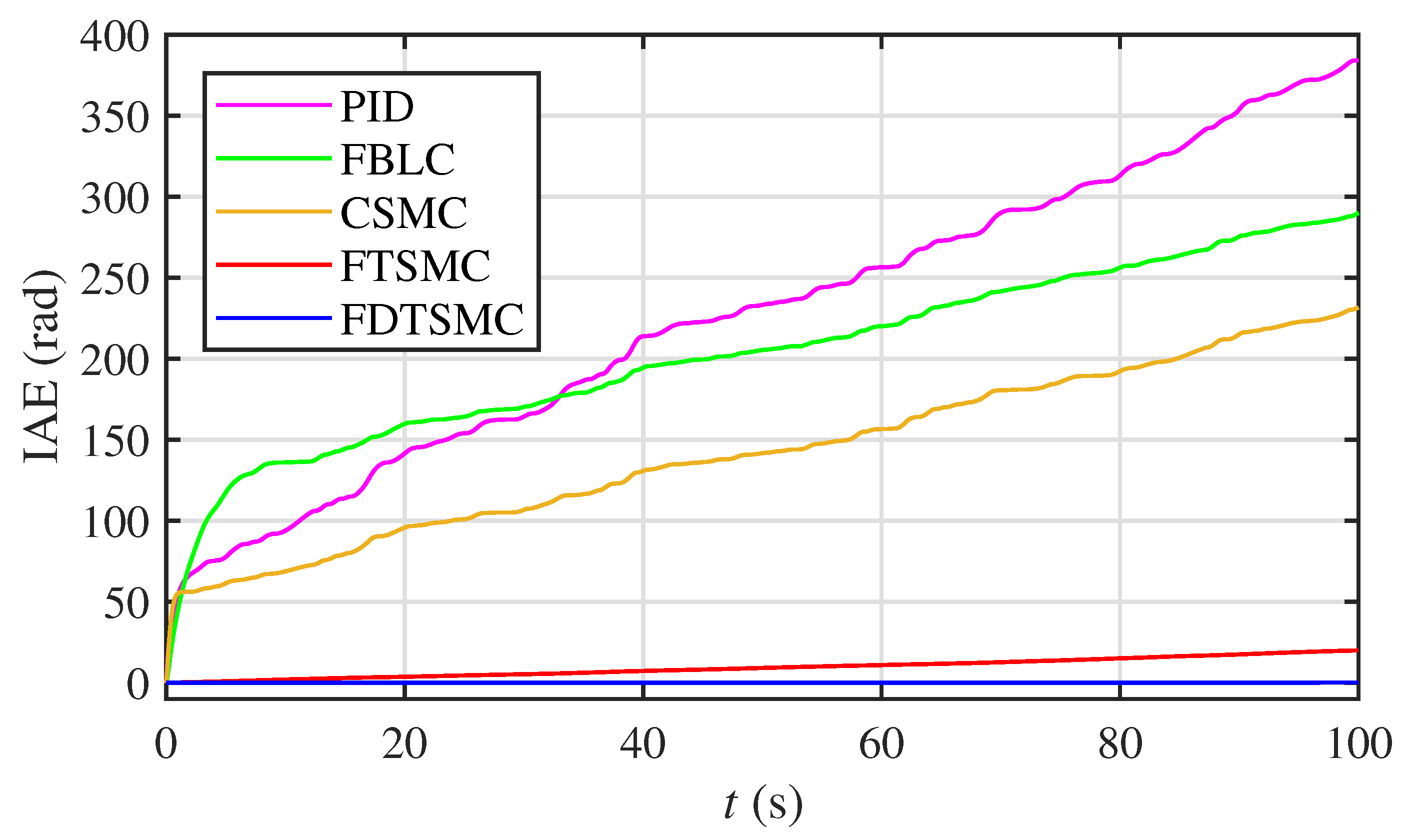
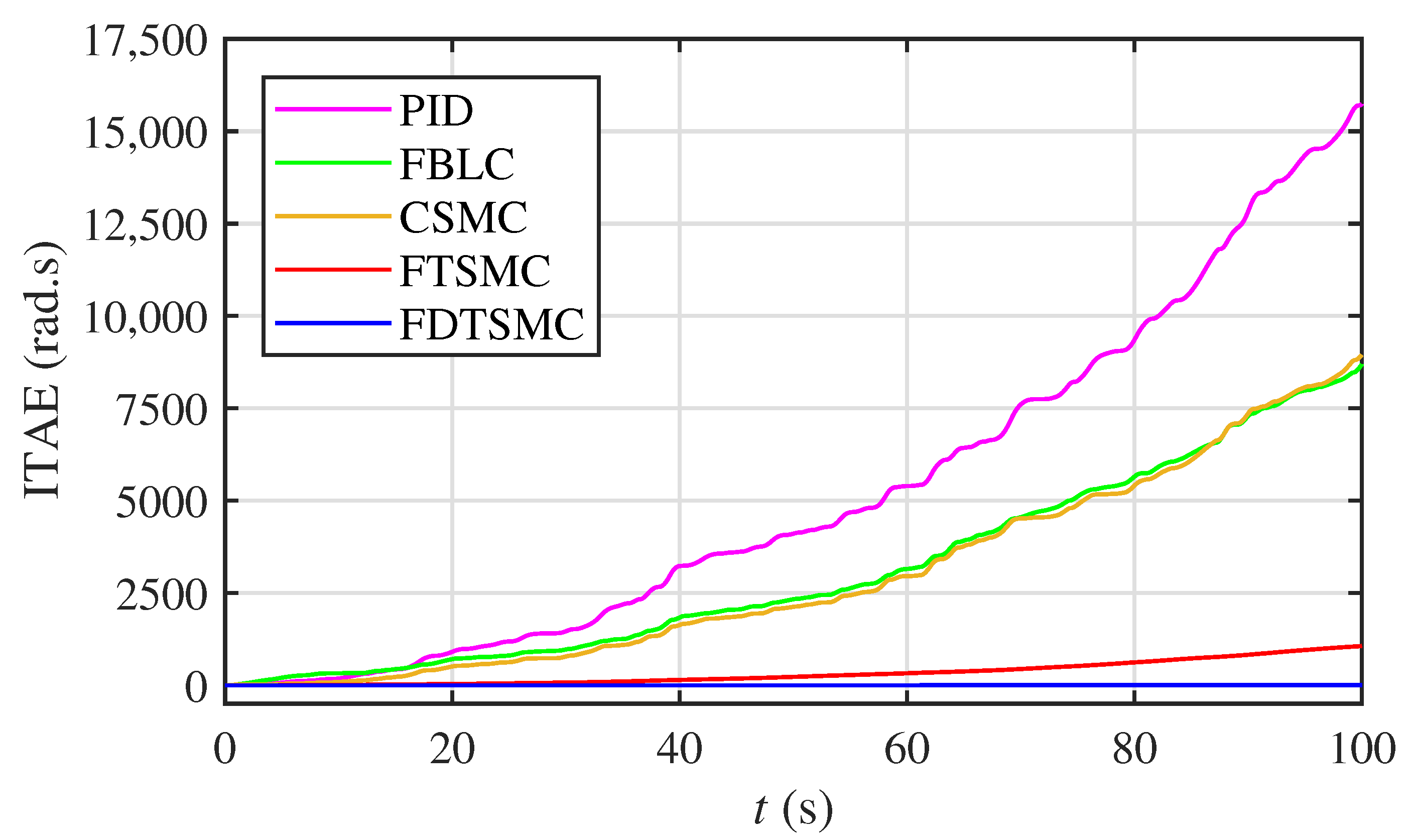
7.2. Performance Indices

To further validate the superior performance of the proposed MPPT strategy to the FTSMC-, CSMC-, FBLC- and PID-based MPPT strategies, the dynamic performance of each MPPT candidate is also evaluated through four different performance indices, given as follows [11,28,29]:

$$\begin{array}{c}ISE={\int }_0^{t_{sim}}{\left[e\left(t\right)\right]}^{2}dt\hfill \\ ITSE={\int }_0^{t_{sim}}t{\left[e\left(t\right)\right]}^{2}dt\hfill \\ IAE={\int }_0^{t_{sim}}\left|e\left(t\right)\right|dt\hfill \\ ITAE={\int }_0^{t_{sim}}t\left|e\left(t\right)\right|dt\hfill \end{array}\}$$

(28)

where $t_{sim}$ indicates the total simulation time.

The performances indices, ISE (integral squared error), ITSE (integral of time squared error), IAE (integral absolute error) and ITAE (integral of time absolute error) have been computed for PMSG–WECS using $e\left(t\right)={\mathrm{\Omega }}_h-{\mathrm{\Omega }}_{ref}$ for each MPPT strategy. It is evident from Figure 15, Figure 16, Figure 17 and Figure 18 that as the time advances, the accumulative error of each MPPT controller also increases. However, the proposed FDTSMC renders the flattest profile and the smallest error in each case, thus guaranteeing its superior performance. Moreover, the FTSMC is the second best MPPT candidate, while the PID is the worst.

8. Conclusions

To extract the maximum possible power from the wind and to reduce chattering, in this research article, a nonlinear MPPT control strategy based on FDTSMC has been proposed for a variable speed, standalone, fixed-pitch, 3 $\mathrm{k}$$\mathrm{W}$ PMSG–WECS. The proposed MPPT strategy has been simulated under a stochastic wind speed profile in MATLAB/Simulink. Its MPPT performance has been compared with and found superior to the FTSMC-, CSMC-, FBLC- and PID-based benchmark MPPT techniques in terms of offering a finite-time convergence, accurate MPPT, low steady-state error, fast dynamic response and minute chattering. The stability of the closed-loop system is demonstrated by the Lyapunov stability theory. The results are promising, and it has been observed that the FDTSMC has the best MPPT performance among the candidates, while the conventional PID has the worst.

References

1. Soliman, M.A.; Hasanien, H.M.; Azazi, H.Z.; El-Kholy, E.E.; Mahmoud, S.A. Linear-quadratic regulator algorithm-based cascaded control scheme for performance enhancement of a variable-speed wind energy conversion system. Arab. J. Sci. Eng. 2019, 44, 2281–2293. [Google Scholar] [CrossRef]
2. Worku, M.Y.; Abido, M.A. Fault Ride-Through and Power Smoothing Control of PMSG-Based Wind Generation Using Supercapacitor Energy Storage System. Arab. J. Sci. Eng. 2019, 44, 2067–2078. [Google Scholar] [CrossRef]
3. Tahir, K.; Belfedal, C.; Allaoui, T.; Denai, M.; Doumi, M.H. A new sliding mode control strategy for variable-speed wind turbine power maximization. Int. Trans. Electr. Energy Syst. 2018, 28, e2513. [Google Scholar] [CrossRef] [Green Version]
4. Housseini, B.; Okou, A.F.; Beguenane, R. Performance comparison of variable speed PMSG-based wind energy conversion system control algorithms. In Proceedings of the 2017 Twelfth International Conference on Ecological Vehicles and Renewable Energies (EVER), Monte-Carlo, Monaco, 11–13 April 2017; pp. 1–10. [Google Scholar]
5. Yaramasu, V.; Dekka, A.; Durán, M.J.; Kouro, S.; Wu, B. PMSG-based wind energy conversion systems: Survey on power converters and controls. IET Electr. Power Appl. 2017, 11, 956–968. [Google Scholar] [CrossRef]
6. Chinchilla, M.; Arnaltes, S.; Burgos, J.C. Control of permanent-magnet generators applied to variable-speed wind-energy systems connected to the grid. IET Electr. Power Appl. 2006, 21, 130–135. [Google Scholar] [CrossRef] [Green Version]
7. Munteanu, I.; Bacha, S.; Bratcu, A.I.; Guiraud, J.; Roye, D. Energy-reliability optimization of wind energy conversion systems by sliding mode control. IEEE Trans. Energy Convers. 2008, 23, 975–985. [Google Scholar] [CrossRef]
8. Shtessel, Y.; Edwards, C.; Fridman, L.; Levant, A. Sliding Mode Control and Observation; Springer: New York, NY, USA, 2014. [Google Scholar]
9. Young, K.D.; Utkin, V.I.; Ozguner, U. A control engineer’s guide to sliding mode control. IEEE Trans. Control Syst. Technol. 1999, 7, 328–342. [Google Scholar] [CrossRef] [Green Version]
10. Liu, J.; Sun, F. A novel dynamic terminal sliding mode control of uncertain nonlinear systems. J. Control Theoryand Appl. 2007, 5, 189–193. [Google Scholar] [CrossRef]
11. Khan, I.U.; Khan, L.; Khan, Q.; Ullah, S.; Khan, U.; Ahmad, S. Neuro-Adaptive Backstepping Integral Sliding Mode Control Design for Nonlinear Wind Energy Conversion System. Turk. J. Electr. Eng. Comput. Sci. 2020, in press. [Google Scholar] [CrossRef]
12. Yazici, İ.; Yaylaci, E.K. Maximum power point tracking for the permanent magnet synchronous generator-based WECS by using the discrete-time integral sliding mode controller with a chattering-free reaching law. IET Power Electron. 2017, 10, 1751–1758. [Google Scholar] [CrossRef]
13. Yin, X.X.; Lin, Y.G.; Li, W.; Liu, H.W.; Gu, Y.J. Fuzzy-logic sliding-mode control strategy for extracting maximum wind power. IEEE Trans. Energy Convers. 2015, 30, 1267–1278. [Google Scholar] [CrossRef]
14. Dursun, E.H.; Kulaksiz, A.A. Second-order sliding mode voltage-regulator for improving MPPT efficiency of PMSG-based WECS. Int. J. Electr. Power Energy Syst. 2020, 121, 106149. [Google Scholar] [CrossRef]
15. Boukattaya, M.; Mezghani, N.; Damak, T. Adaptive nonsingular fast terminal sliding-mode control for the tracking problem of uncertain dynamical systems. ISA Trans. 2018, 77, 1–19. [Google Scholar] [CrossRef]
16. El Mourabit, Y.; Derouich, A.; El Ghzizal, A.; El Ouanjli, N.; Zamzoum, O. Nonlinear backstepping control for PMSG wind turbine used on the real wind profile of the Dakhla-Morocco city. Int. Trans. Electr. Energy Syst. 2020, 30, e12297. [Google Scholar] [CrossRef]
17. Munteanu, I.; Bratcu, A.I.; Cutululis, N.A.; Ceangǎ, E. Optimal Control of Wind Energy Systems: Towards a Global Approach; Springer: London, UK, 2008. [Google Scholar]
18. Cutululis, N.A.; Ceangǎ, E.; Hansen, A.D.; Sørensen, P. Robust multi-model control of an autonomous wind power system. Wind Energy 2006, 9, 399–419. [Google Scholar] [CrossRef]
19. Cheikh, R.; Menacer, A.; Alaoui, L.C.; Drid, S. Robust nonlinear control via feedback linearization and Lyapunov theory for permanent magnet synchronous generator-based wind energy conversion system. Front. Energy 2020, 14, 180–191. [Google Scholar] [CrossRef]
20. Slotine, J.J.E.; Li, W. Applied Nonlinear Control; Prentice Hall: Englewood Cliffs, NJ, USA, 1991. [Google Scholar]
21. Marquez, H.J. Nonlinear Control Systems; John Wiley & Sons: Hoboken, NJ, USA, 2003. [Google Scholar]
22. Lau, C.K.; Ghosh, K.; Hussain, M.A.; Hassan, C.C. Fault diagnosis of Tennessee Eastman process with multi-scale PCA and ANFIS. Chemom. Intell. Lab. Syst. 2013, 120, 1–14. [Google Scholar] [CrossRef]
23. Zhihong, M.; Paplinski, A.P.; Wu, H.R. A robust MIMO terminal sliding mode control scheme for rigid robotic manipulators. IEEE Trans. Autom. Control 1994, 39, 2464–2469. [Google Scholar] [CrossRef]
24. Yu, X.; Zhihong, M. Fast terminal sliding-mode control design for nonlinear dynamical systems. IEEE Trans. Circuits Syst. I Fundam. Theory Appl. 2002, 49, 261–264. [Google Scholar]
25. Ziong, J.J.; Zhang, G.B. Global fast dynamic terminal sliding mode control for a quadrotor UAV. ISA Trans. 2017, 66, 233–240. [Google Scholar]
26. Dursun, E.H.; Kulaksiz, A.A. Second-Order Fast Terminal Sliding Mode Control for MPPT of PMSG-based Wind Energy Conversion System. Elektron. Elektrotech. 2020, 26, 39–45. [Google Scholar] [CrossRef]
27. Soufi, Y.; Kahla, S.; Bechouatb, M. Feedback linearization control based particle swarm optimization for maximum power point tracking of wind turbine equipped by PMSG connected to the grid. Int. J. Hydrogen Energy 2016, 41, 20950–20955. [Google Scholar] [CrossRef]
28. Sahib, M.A.; Ahmed, B.S. A new multiobjective performance criterion used in PID tuning optimization algorithms. J. Adv. Res. 2016, 7, 125–134. [Google Scholar] [CrossRef] [Green Version]
29. Ali, K.; Khan, Q.; Ullah, S.; Khan, I.; Khan, L. Nonlinear robust integral backstepping based MPPT control for stand-alone photovoltaic system. PLoS ONE 2020, 15, e0231749. [Google Scholar] [CrossRef] [PubMed]
Figure 1. Schematic of the overall variable speed permanent magnet synchronous generator–wind energy conversion system (PMSG–WECS).
Applsci 10 06361 g001
Figure 2. Wind turbine mechanical power output under different wind speeds.
Applsci 10 06361 g002
Figure 3. ANFIS network structure for PMSG–WECS Lie-derivatives estimation.
Applsci 10 06361 g003
Figure 4. Computational flow chart for implementation of the proposed MPPT strategy.
Applsci 10 06361 g004
Figure 5. Closed-loop control system for the PMSG–WECS.
Applsci 10 06361 g005
Figure 6. High-speed shaft rotational speed tracking.
Applsci 10 06361 g006
Figure 7. High-speed shaft rotational speed tracking error.
Applsci 10 06361 g007
Figure 8. Tip speed ratio performance.
Applsci 10 06361 g008
Figure 9. Power conversion coefficient.
Applsci 10 06361 g009
Figure 10. Low-speed shaft mechanical power versus the tip speed ratio.
Applsci 10 06361 g010
Figure 11. High-speed shaft mechanical power versus the tip speed ratio.
Applsci 10 06361 g011
Figure 12. Mechanical power versus the low-speed shaft rotational speed.
Applsci 10 06361 g012
Figure 13. Electromagnetic torque versus the tip speed ratio performance.
Applsci 10 06361 g013
Figure 14. Mechanical torque versus the low-speed shaft rotational speed.
Applsci 10 06361 g014
Figure 15. Integral squared error.
Applsci 10 06361 g015
Figure 16. Integral of time squared error.
Applsci 10 06361 g016
Figure 17. Integral absolute error.
Applsci 10 06361 g017
Figure 18. Integral of time absolute error.
Applsci 10 06361 g018