Augmented Tikhonov Regularization Method for Dynamic Load Identification

Abstract

We introduce the augmented Tikhonov regularization method motivated by Bayesian principle to improve the load identification accuracy in seriously ill-posed problems. Firstly, the Green kernel function of a structural dynamic response is established; then, the unknown external loads are identified. In order to reduce the identification error, the augmented Tikhonov regularization method is combined with the Green kernel function. It should be also noted that we propose a novel algorithm to determine the initial values of the regularization parameters. The initial value is selected by finding a local minimum value of the slope of the residual norm. To verify the effectiveness and the accuracy of the proposed method, three experiments are performed, and then the proposed algorithm is used to reproduce the experimental results numerically. Numerical comparisons with the standard Tikhonov regularization method show the advantages of the proposed method. Furthermore, the presented results show clear advantages when dealing with ill-posedness of the problem.

1. Introduction

The dynamic loads acting on a structure cannot be directly measured in many cases, and it is necessary to use indirect methods. Among such methods, retrieving the actual dynamic loads by measuring the vibration response of a structure has attracted a wide attention. In this case, the dynamic load identification problem involves solving an ill-posed inverse problem. Hence, any small amount of measurement noise causes a huge disturbance of identification results. For example, it is common to have small singular values due to the measurement accuracy error. Although such values are often very small, the ill-posedness of the problem makes it difficult to get the correct solution. In general, the solution accuracy is often affected by an order of magnitude compared to the error in the measurement accuracy.

Many researchers investigated the ill-posedness problem, and several approaches were proposed [1,2,3,4,5,6,7,8]. In principle, these approaches are always based on regularization methods. For example, the Tikhonov regularization method can be used to identify the impact load, employing the frequency response function and the strain response of an experimental system [9]. Tikhonov regularization method, based on ordinary cross validation (OCV) [10], is also used to identify the excitation acting on a thin plate structure. The presented results show the robustness of Tikhonov regularization method when compared to the truncated singular value decomposition method. In another work, three regularization parameters, namely OCV, generalized cross validation (GCV), and L-curve method, are studied [11]. It is shown that the L-curve method combined with Tikhonov regularization method leads to better accuracy for a given level of noise in the measurement data. In order to improve the noise immunity and robustness, a new regularization parameter was introduced and verified by numerical and experiment tests [12]. The quotient function method was also proposed for selecting the optimal regularization parameters [13]. Unlike the GCV and the L-curve methods, the proposed method is applicable to load identification in resonant, as well as non-resonant, regimes. However, the load reconstruction in the traditional Tikhonov regularization method can often be inefficient, especially in larger problems. To deal with this issue, new regularization methods, such as sparse regularization, are proposed. An example is the sparse convex optimization model, which is established for load identification using the basis functions [14]. The effectiveness of the sparse regularization for harmonic, as well as impact loads, identification is confirmed using experimental results for a thin-plate cantilever structure.

The Tikhonov regularization method remains the most widely used method for dynamic load identification [15]. However, the matching L-curve and GCV regularization parameter selection method may fail when L-curve is too smooth, without inflection points, or GCV function curve is too flat at the minimum value. In these cases, it is difficult to accurately locate the regularization parameter, and an unsuitable parameter will lead to a large error in the load identification. To overcome this limitation, Bayesian principle is implemented to produce the augmented Tikhonov regularization method. The main idea is to transform the ill-posed problem into an optimization problem so that the optimal solution is the solution of the ill-posed problem. The augmented Tikhonov regularization method is first applied to solve inverse problems of general partial differential equations [16] and then implemented in heat transfer applications to identify a heat source [17]. The load identification based on the Bayesian principle has improved accuracy and wide applications when compared to the standard Tikhonov regularization method. However, so far, the studies on the optimization problem to be solved are based on maximizing/minimizing a posteriori estimate of the Bayesian formulation, which only takes into account given initial parameters but not the optimal initial parameters [18,19,20,21,22]. Considering the impact of optimal initial values, selection for the regularization parameters can be vital for solving ill-posedness in dynamic load identification. However, there are no available methods to determine the initial values. Without the optimal initial values, it may become impossible to obtain the accurate identification results. Thus, for the augmented Tikhonov regularization method, it is critical to define a method for selecting optimal initial values.

Since the Green kernel function can be used to construct the dynamic load identification model [23]. This paper introduces the augmented Tikhonov regularization method in combination with the Green kernel function in dynamic load identification. It also proposes a new parameters selection method for the augmented Tikhonov regularization initial parameters, and the accuracy is compared to the standard Tikhonov regularization method. The paper proceeds as follows: the load identification model using Green kernel function is deduced in Section 2; in Section 3, the augmented Tikhonov regularization method in dynamic load identification is presented, while the new parameters selection method is proposed in Section 4. Next, in Section 5, three numerical examples are conducted to study the efficiency, as well as the accuracy, of the augmented Tikhonov regularization method under different loads with different noise conditions. In Section 6, the augmented Tikhonov regularization method is used to identify the load in an experimental setting of simply supported beams. We finish with some concluding remarks in Section 7.

2. Green Kernel Function

For a multi-degrees-of-freedom system, the general vibration differential equation is often written as

$$\{\begin{array}{l}\mathit{M}\ddot{\mathit{x}}(t)+\mathit{C}\dot{\mathit{x}}(t)+\mathit{K}\mathit{x}(t)=\mathit{f}(t)\\ \mathit{x}(0)={\mathit{x}}_0,\dot{\mathit{x}}(0)={\dot{\mathit{x}}}_0\end{array}.$$

(1)

Here, $\mathit{M},\mathit{K}\mathit{,}\mathit{C}$ are the mass, stiffness and damping matrix of the system, respectively, while $\mathit{x},\dot{\mathit{x}},\ddot{\mathit{x}}$ are the displacement, the velocity, and the acceleration vectors of the system response. The variable $\mathit{f}$ represents external forces acting on the system. Assuming a zero initial state, i.e., $x_0$ and ${\dot{x}}_0$ are both zero, the displacement response of the i-th degree of freedom is

$$x_i\left(t\right)={\displaystyle \sum _{j=1}^n{x}_{ij}\left(t\right)}={\displaystyle \sum _{j=1}^n{\displaystyle {\int }_0^t{h}_{ij}\left(t-\tau \right)}}{f}_j\left(\tau \right)d\tau ,$$

(2)

where $x_{ij}\left(t\right)$ is the displacement response of i-th degree of freedom caused by the external force acting on the j-th degree, and $h_{ij}$ is the unit impulse response function, while $f_j$ represents the external force acting on the j-th degree of freedom.

Assuming the sampling interval of the response is $\Delta t$, $x_{ij}$ can be simplified using integral discretization

$$x_{ij}(n\Delta t)\approx \left[{\displaystyle \sum _{i=0}^{n-1}h(t-i\Delta t)f(i\Delta t)}\right]\Delta t.$$

(3)

Rewrite Equation (3) into matrix form as

$$\left[\begin{array}{c}{x}_{ij}\left(1\right)\\ x_{ij}\left(2\right)\\ ⋮\\ x_{ij}\left(m\right)\end{array}\right]=\left[\begin{array}{cccc}{h}_{ij}\left(1\right)& & & \\ h_{ij}\left(2\right)& h_{ij}\left(1\right)& & \\ ⋮& ⋮& \ddots & \\ h_{ij}\left(m\right)& h_{ij}\left(m-1\right)& \cdots & h_{ij}\left(1\right)\end{array}\right]\left[\begin{array}{c}{f}_j\left(0\right)\\ f_j\left(1\right)\\ ⋮\\ f_j\left(m-1\right)\end{array}\right]\Delta t.$$

(4)

Equation (4) can be abbreviated as

$${\mathit{Y}}_{ij}={\mathit{H}}_{ij}{\mathit{F}}_j.$$

(5)

Here, $Y_{ij}$ is a discrete vector form of $x_{ij}$, while $F_j$ is a discrete vector form of $f_j$. When only one load is acting on the system, i.e., on the j-th degree of freedom, the response of the i-th degree of freedom can be expressed as

$${\mathit{Y}}_i={\mathit{Y}}_{ij}={\mathit{H}}_{ij}{\mathit{F}}_j.$$

(6)

Equation (6) is the linear equations in the case of a single input and a single output. The unknown force $F_j$ can be obtained by solving Equation (6). Here, $H_{ij}$ is the kernel function matrix. When there are $M$ loads acting on different degrees of freedom, the number of the responses to be collected $N$ needs to meet the following formula $M\le N$. Thus, the relationship between $M$ loads and $N$ responses can be obtained:

$$\begin{array}{ccc}{\mathit{Y}}_i={\displaystyle \sum _{j=1}^M{\mathit{Y}}_{ij}}={\displaystyle \sum _{j=1}^M{\mathit{H}}_{ij}{\mathit{F}}_j}& & (i=1,2,\cdots ,N)\end{array}.$$

(7)

Rewrite Equation (7) in matrix form as

$$\left[\begin{array}{c}{\mathit{Y}}_1\\ {\mathit{Y}}_2\\ ⋮\\ {\mathit{Y}}_N\end{array}\right]=\left[\begin{array}{cccc}{\mathit{H}}_{11}& {\mathit{H}}_{12}& \cdots & {\mathit{H}}_{1M}\\ {\mathit{H}}_{21}& {\mathit{H}}_{22}& \cdots & {\mathit{H}}_{2M}\\ ⋮& ⋮& & ⋮\\ {\mathit{H}}_{N1}& {\mathit{H}}_{N2}& \cdots & {\mathit{H}}_{NM}\end{array}\right]\left[\begin{array}{c}{\mathit{F}}_1\\ {\mathit{F}}_2\\ ⋮\\ {\mathit{F}}_M\end{array}\right].$$

(8)

Equation (8) is the linear equations in the case of multiple inputs and outputs, and the unknown force $F_1,F_2,\cdots ,F_M$ can be obtained by solving this equation. Clearly, Equations (6) and (8) both conform to the form of $\mathit{y}=\mathit{H}\mathit{f}$. The inversion of equations in this form usually introduces a significant error into the solution due to the ill-posedness of the problem that is caused by the ill-posedness of the kernel function matrix $\mathit{H}$, especially for large systems, i.e., hundreds of degrees of freedom. Next, we discuss reducing the ill-posedness problem using Augmented Tikhonov regularization method.

3. Augmented Tikhonov Regularization Method

The augmented Tikhonov regularization is an application of the Bayesian principle in the field of inverse problems. The basic idea of the Bayesian theory is to obtain the posterior probability density function through the likelihood function and the prior probability density function, and then estimate the unknown quantity according to the posterior probability density.

In the model $\mathit{y}=\mathit{H}\mathit{f}$ mentioned above, the output signal $\mathit{y}$ will always contain some noise ${\mu }$.

$$\mathit{y}=\mathit{H}\mathit{f}+\mathbf{\mu }.$$

(9)

According to the Bayesian principle, the posterior probability density function of the unknown quantity $\mathit{f}$ can be obtained:

$$p(\mathit{f}|\mathit{y})\propto p(\mathit{f})p(\mathit{y}|\mathit{f}),$$

(10)

where $p(\mathit{f}|\mathit{y})$ is the posterior probability density function, while $p(\mathit{f})$ is the prior probability density function. The variable $p(\mathit{y}|\mathit{f})$ is the likelihood function. Thus, the loads $\mathit{f}$ can be estimated by the maximum posterior probability density function:

$${\widehat{\mathit{f}}}_{map}=\arg \underset{\mathit{y}}{\max } p(\mathit{f}|\mathit{y}).$$

(11)

The likelihood function represents the probability density function of $\mathit{y}$ when the random variable $\mathit{f}$ is given. The form of the likelihood function is generally determined by the noise $\mu$. Usually, the white Gaussian noise with a zero mean and a standard deviation of $\sigma$ can provide a proper representation for $\mu$. The noise likelihood function can then be represent as

$$p(\mathit{y}|\mathit{f})\propto {({\sigma }^2)}^{-n/2}\exp (-\frac{{\Vert \mathit{H}\mathit{f}-\mathit{y}\Vert }_2^2}{2{\sigma }^2}),$$

(12)

where n is the data length of $\mathit{y}$.

The above probability density function needs to be selected according to the empirical method. In this study, Markov random field is selected as the prior model.

$$p(\mathit{f})\propto \exp (-\sum _{i~j}{\mathit{W}}_{ij}\varphi (\gamma (f_i-f_j))),$$

(13)

where $\gamma$ is a magnification factor, while $\varphi (\gamma (f_i-f_j))$ is a non-negative function that determines the specific form of this Markov field, and ${\mathit{W}}_{ij}$ is a non-negative weight coefficient. The function $\varphi$ is then set to the form $\varphi (t)=1/2t^2$, so that the Markov random field is

$$p(\mathit{f})\propto {\lambda }^{m/2}\exp (-\frac{1}{2}\lambda {\mathit{f}}^T\mathit{W}\mathit{f}),$$

(14)

where the variable $\lambda$ denotes the scaling parameter, and $m$ the dimension of vector $\mathit{f}$. $\mathit{W}$ represents the symmetric matrix composed of ${\mathit{W}}_{ij}$. The posterior probability density function can be obtained by substituting Equations (12) and (14) into Equation (10), and the following is obtained:

$$p(\mathit{f}|\mathit{y})\propto {({\sigma }^2)}^{-n/2}{\lambda }^{m/2}\exp (-\frac{{\Vert \mathit{H}\mathit{f}-\mathit{y}\Vert }_2^2}{2{\sigma }^2})\exp (-\frac{1}{2}\lambda {\mathit{f}}^T\mathit{W}\mathit{f}).$$

(15)

In the Bayesian hierarchical model, the two unknown parameters $\lambda ,\sigma$ in Equation (15) can be regarded as random variables; hence, they play the role of regularization parameters. For convenience, we set $\tau =1/{\sigma }^2$. The prior distributions of $\lambda ,\tau$ are assumed to be a Gamma distribution.

$$p(\lambda )=\frac{{\beta }_1^{{\alpha }_1}}{\Gamma ({\alpha }_1)}{\lambda }^{{\alpha }_1-1}\exp (-{\beta }_1\lambda ),$$

(16)

$$p(\tau )=\frac{{\beta }_2^{{\alpha }_2}}{\Gamma ({\alpha }_2)}{\tau }^{{\alpha }_2-1}\exp (-{\beta }_2\tau ),$$

(17)

where ${\alpha }_1,{\beta }_1,{\alpha }_2,{\beta }_2$ are the parameters of the Gamma distribution. Meanwhile, due to the introduction of two new random variables, the likelihood function and the prior probability density function are different from the previous ones.

$$p(\mathit{y}|\mathit{f},\tau )\propto {\tau }^{n/2}\exp (-\frac{\tau }{2}{\Vert \mathit{H}\mathit{f}-\mathit{y}\Vert }_2^2),$$

(18)

$$p(\mathit{f}|\lambda )\propto {\lambda }^{m/2}\exp (-\frac{1}{2}\lambda {\Vert \mathit{f}\Vert }_2^2).$$

(19)

Then, the joint posterior probability density function can be obtained

$$p(\mathit{f},\lambda ,\tau |\mathit{y})\propto p(\mathit{y}|\mathit{f},\tau )p(\mathit{f}|\lambda )p(\tau )p(\lambda ).$$

(20)

Substitute Equations (16)–(19) into Equation (20), and we can obtain the specific expression

$$p(\mathit{f},\lambda ,\tau |\mathit{y})\propto {\tau }^{n/2+{\alpha }_2-1}{\lambda }^{m/2+{\alpha }_1-1}\exp (-\frac{\tau }{2}{\Vert \mathit{H}\mathit{f}-\mathit{y}\Vert }_2^2-\frac{1}{2}\lambda {\Vert \mathit{f}\Vert }_2^2-{\beta }_1\lambda -{\beta }_2\tau ).$$

(21)

The values of $\mathit{f},\lambda ,\tau$ can be estimated simultaneously by maximizing Equation (21). In order to facilitate the solution, we convert the Equation (21) into the minimum value of the following formula by using the negative form of the log-likelihood function:

$$\ln L(\mathit{f},\lambda ,\tau )=\frac{\tau }{2}{\Vert \mathit{H}\mathit{f}-\mathit{y}\Vert }_2^2+\frac{\lambda }{2}{\Vert \mathit{f}\Vert }_2^2-(\frac{n}{2}+{\alpha }_2-1)\ln \tau -(\frac{m}{2}+{\alpha }_1-1)\ln \lambda +{\beta }_1\lambda +{\beta }_2\tau .$$

(22)

The alternating direction algorithm is used to solve the minimum problem in this study. The solution steps are as follows:

• Calculate the partial derivatives of log-likelihood function with respect to the variables $\mathit{f},\lambda ,\tau$ respectively, and let them vanish.

  $$\frac{\partial lnL(\mathit{f},\lambda ,\tau )}{\partial \mathit{f}}=({\mathit{H}}^{{\rm T}}\mathit{H}+\frac{\lambda }{\tau }\mathit{I})\mathit{f}-{\mathit{H}}^{{\rm T}}\mathit{y}=0,$$

  (23)

  $$\frac{\partial lnL(\mathit{f},\lambda ,\tau )}{\partial \tau }=\frac{n+2{\alpha }_2-2}{\tau }-{\Vert \mathit{H}\mathit{f}-\mathit{y}\Vert }_2^2-2{\beta }_2=0,$$

  (24)

  $$\frac{\partial lnL(\mathit{f},\lambda ,\tau )}{\partial \lambda }=\frac{m+2{\alpha }_1-2}{\lambda }-{\Vert \mathit{f}\Vert }_2^2-2{\beta }_1=0.$$

  (25)
• Three formulas can be obtained from the above formulas:

  $$\mathit{f}={({\mathit{H}}^{{\rm T}}\mathit{H}+\frac{\lambda }{\tau }\mathit{I})}^{-1}{\mathit{H}}^{{\rm T}}\mathit{y},$$

  (26)

  $$\lambda =\frac{m+2{\alpha }_1-2}{{\Vert \mathit{f}\Vert }_2^2+2{\beta }_1},$$

  (27)

  $$\tau =\frac{n+2{\alpha }_2-2}{{\Vert \mathit{H}\mathit{f}-\mathit{y}\Vert }_2^2+2{\beta }_2}.$$

  (28)
• The unknown force $\mathit{f}$ can be calculated by setting appropriate initial values and repeating iterative Equations (26)–(28).

The flow chart are shown in the Figure 1, and specific iteration steps are:

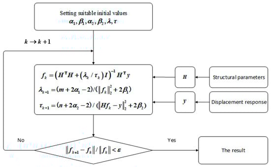
Figure 1. Load identification flow chart.

• Set suitable initial values ${\alpha }_1,{\beta }_1,{\alpha }_2,{\beta }_2,\lambda ,\tau$, and $k=1$ (this step is discussed next);
• Calculate ${\mathit{f}}_k$: ${\mathit{f}}_k={\left({\mathit{H}}^{{\rm T}}\mathit{H}+\left({\lambda }_k/{\tau }_k\right)\mathit{I}\right)}^{-1}{\mathit{H}}^{{\rm T}}\mathit{y}$;
• Calculate new ${\lambda }_{k+1}$ and ${\tau }_{k+1}$:

  $$\begin{array}{ccc}{\lambda }_{k+1}=\frac{m+2{\alpha }_1-2}{{\Vert {\mathit{f}}_k\Vert }_2^2+2{\beta }_1}& & {\tau }_{k+1}=\frac{n+2{\alpha }_2-2}{{\Vert \mathit{H}{\mathit{f}}_k-\mathit{y}\Vert }_2^2+2{\beta }_2}\end{array};$$
• Set $k=k+1$, and return to step (2) to repeat the iterative calculation until the termination condition is met. The termination condition in this study is $\Vert {\mathit{f}}_{k+1}-{\mathit{f}}_k\Vert /\Vert {\mathit{f}}_k\Vert <\epsilon$, where $\epsilon$ is $1\times {10}^{-8}$.

4. Initial Parameters Selection

As discussed above, the solution with augmented Tikhonov regularization method, six initial parameters need to be defined. Among these, the values of $\lambda$ and $\tau$ changes after each iteration, while those of ${\alpha }_1,{\beta }_1,{\alpha }_2,{\beta }_2$ do not. In order to understand the effect of the initial values of $\lambda ,\tau$, we run hundreds of simulations, where we noticed that the initial values of these parameters have little effect on the load identification algorithm. We also noticed that setting the parameters ${\alpha }_1,{\alpha }_2$ close to unity leads to stable results with accurate load identification. However, the choice of ${\beta }_1,{\beta }_2$ may lead to a significant change in the identification results. Therefore, in the following, we limit our discussion to the selection of these two parameters.

The correlation coefficient (r) and relative error (RE) are used to estimate the load identification error in this paper. These are calculated as follows:

$$r=\frac{{\displaystyle \sum _{i=1}^n[{\mathit{f}}_{iden}(\mathrm{i})-{\overline{\mathit{f}}}_{iden}][{\mathit{f}}_{true}(\mathrm{i})-{\overline{\mathit{f}}}_{true}]}}{\Vert {\mathit{f}}_{iden}-{\overline{f}}_{iden}\Vert \cdot \Vert {\mathit{f}}_{true}-{\overline{\mathit{f}}}_{true}\Vert }\times 100\%,$$

(29)

$$RE=\frac{\Vert {\mathit{f}}_{iden}(i)-{\mathit{f}}_{true}(i)\Vert }{\Vert {\mathit{f}}_{true}(i)\Vert }\times 100\%,$$

(30)

where ${\mathit{f}}_{iden}$ is the identified force, and ${\mathit{f}}_{true}$ is the true force, while ${\overline{\mathit{f}}}_{iden}$ and ${\overline{\mathit{f}}}_{true}$ are the means of ${\mathit{f}}_{iden}$ and ${\mathit{f}}_{true}$, respectively.

The values of ${\beta }_1,{\beta }_2$ can have a significant impact on the load identification results ${\Vert {\mathit{f}}_k\Vert }_2^2$ and the residual norm ${\Vert \mathit{H}{\mathit{f}}_k-\mathit{y}\Vert }_2^2$. To analyze the impact of selecting the values of ${\beta }_1,{\beta }_2$ on the load identification, we study, in this section, a single degree of freedom system. The considered parameters for this system are $m=1\mathrm{kg}$, $k=1500\mathrm{N}/\mathrm{m}$ and $c=15\mathrm{N}·\mathrm{s}/\mathrm{m}$. The load applied on the system is periodic defined by $F=100*\sin (\pi *50*t)$. We also set the parameters ${\alpha }_1,{\alpha }_2$ to 2, which is relatively a small value while the parameters $\lambda ,\tau$ are set to 100 and $1\times {10}^{12}$, respectively. To understand the effect of the parameters ${\beta }_1$ and ${\beta }_2$ on the identified load, their values will be varied, and the identified load will be recorded.

Figure 2 shows the changes in the correlation coefficient and the relative error for varying the values of ${\beta }_1,{\beta }_2$ when the signal noise ratio (SNR) of the response is 30 dB. It can be seen in the figure that the optimum range of values for ${\beta }_1$ is from 10⁻⁵ to 10⁵, and, for ${\beta }_2$, is a narrow band close to 10⁴. In this range, the correlation coefficient is close to 1, while the relative error is close to 0. This suggests that the load identification accuracy is higher at this specific range of parameters ${\beta }_1,{\beta }_2$. Clearly, the optimum range for ${\beta }_1$ is much wider compared to ${\beta }_2$. Thus, choosing an optimum value for ${\beta }_2$ is our next concern.

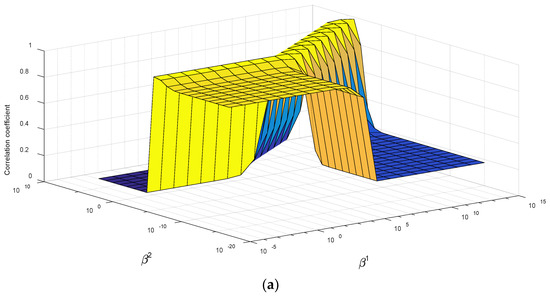
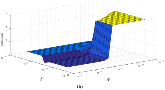
Figure 2. (a) Correlation coefficient varies with the ${\beta }_1,{\beta }_2$. (b) Relative error varies with the ${\beta }_1,{\beta }_2$.

In real world applications, because the load acting on the structures is unknown, it is not possible to define the correlation coefficient and the relative error. Therefore, to determine the optimum values for the parameter ${\beta }_2$, we use the relation between the parameter ${\beta }_2$ and the residual norm $\left|\right|Hf-y{\left|\right|}_2^2$ of the identified load. Indeed, in the load identification process, we rebuild the dynamic responses according to the identified load for a given parameter ${\beta }_2$ and then calculate the residual norm $\left|\right|Hf-y{\left|\right|}_2^2$. When the noise level of the dynamic responses is known, we can find the optimum ${\beta }_2$ by comparing the real residual norm with the computation residual norm, which is shown in Figure 3a. When the real noise level is not available, we calculate the slope of the residual norm $\left|\right|Hf-y{\left|\right|}_2^2$ with respect to ${\beta }_2$ and then take the local minimum value as the optimum point of the parameter ${\beta }_2$, as shown in Figure 3b.

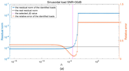
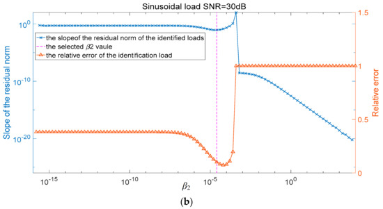
Figure 3. (a) ${\beta }_2$ selection with the response noise level known. (b) ${\beta }_2$ selection with the response noise level unknown.

In Figure 3, the blue curve represents the slope of the residual norm, while the red curve represents the relative error of the identification load. The black curve gives the real residual norm according to the response noise level. The pink vertical curve represents the selected ${\beta }_2$ value corresponding to the minimum slope point of the residual norm. The red curve shows that the load identification error is ideal with the selected ${\beta }_2$ value. It should be pointed out, in this case, that the response noise level is 30 dB (SNR). Based on the above parametric study, we choose the following values for ${\alpha }_1,{\beta }_1,{\alpha }_2,\lambda ,\tau ,$ $2.1\times {10}^{-5},2100,1\times {10}^{12}$, respectively, while ${\beta }_2$ is determined according to the selection method shown in Figure 3.

5. Numerical Results

In order to study the efficiency and the accuracy of the proposed augmented Tikhonov regularization method on dynamic load identification, three numerical simulation examples are studied. These include two multi-degrees-of-freedom system examples and a cantilever beam example.

5.1. Single Force Identification Simulation

We first aim to identify the load applied on a four-degrees-of-freedom system. The system is shown in Figure 4, and the system parameters are listed underneath.

$$\begin{array}{l}{m}_1=m_2=m_3=m_4=10\mathrm{kg}\\ k_1=k_2=k_3=k_4=k_5=5000\mathrm{N}/\mathrm{m}\\ c_1=c_2=c_3=c_4=c_5=100\mathrm{N}·\mathrm{s}/\mathrm{m}\end{array}$$

(31)

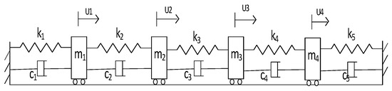
Figure 4. Four-degree-of-freedom system.

The regularization parameters are obtained following the procedure described in Section 4. Three types of force are studied: simple harmonic excitation, triangular wave excitation, and impact load. The load is only applied to the first degree of freedom. We assume the system initially has a stationary state, i.e., zero initial conditions. The sampling time interval is 0.001 s. The considered time span is 0.5 s. The load identification results of the three loads with the SNR of 40 dB, 30 dB, and 20 dB are shown in Figure 5, Figure 6, Figure 7, Figure 8, Figure 9, Figure 10, Figure 11, Figure 12 and Figure 13. On the left side of these figures, we show the results obtained with the Tikhonov regularization method, and, on the right, we show the result of the proposed augmented Tikhonov regularization method. The identification result errors are shown in Table 1.

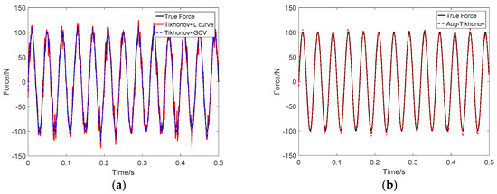
Figure 5. Identification result of sinusoidal load at SNR 40 dB: (a) Tikhonov method; (b) the proposed method.

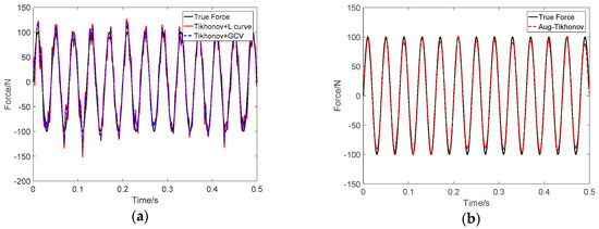
Figure 6. Identification result of sinusoidal load at SNR 30 dB: (a) Tikhonov method; (b) the proposed method.

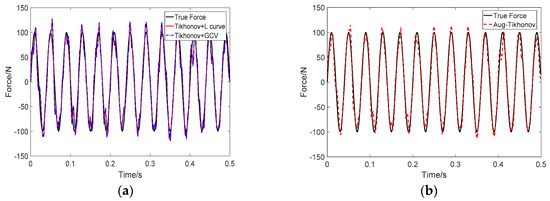
Figure 7. Identification result of sinusoidal load at SNR 20 dB: (a) Tikhonov method; (b) the proposed method.

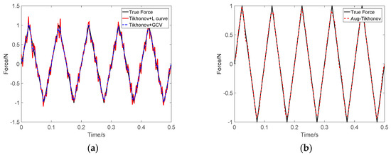
Figure 8. Identification result of triangle wave load at SNR 40 dB: (a) Tikhonov method; (b) the proposed method.

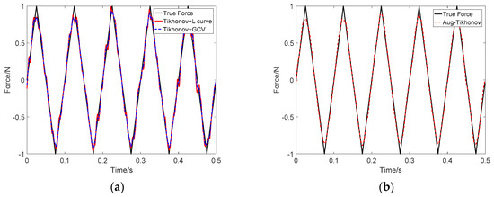
Figure 9. Identification result of triangle wave load at SNR 30 dB: (a) Tikhonov method; (b) the proposed method.

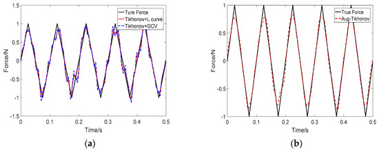
Figure 10. Identification result of triangle wave load at SNR 20 dB: (a) Tikhonov method; (b) the proposed method.

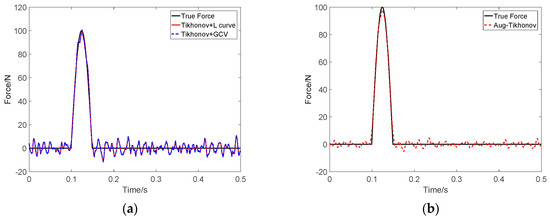
Figure 11. Identification result of impact load at SNR 40 dB: (a) Tikhonov method; (b) the proposed method.

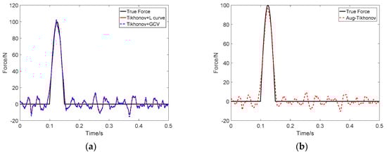
Figure 12. Identification result of impact load at SNR 30 dB: (a) Tikhonov method; (b) the proposed method.

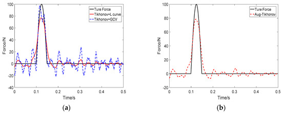
Figure 13. Identification result of impact load at SNR 20 dB: (a) Tikhonov method; (b) the proposed method.

Table 1. Force identification results error of four-degree-of-freedom system.

Force	SNR	Tikhonov + L Curve		Tikhonov + GCV		Augmented Tikhonov
		r	RE	r	RE	r	RE
sinusoidal load	40	87.83%	20.50%	95.30%	11.25%	99.74%	7.18%
	30	82.34%	23.01%	89.10%	18.21%	99.84%	7.94%
	20	96.93%	22.31%	90.44%	23.58%	98.30%	18.38%
Triangle load	40	90.99%	18.13%	97.50%	8.87%	99.82%	6.03%
	30	97.25%	12.69%	99.50%	9.42%	99.65%	8.43%
	20	98.29%	17.86%	96.55%	23.41%	99.18%	14.06%
Impact load	40	97.91%	16.58%	96.03%	16.58%	99.64%	8.47%
	30	96.16%	21.04%	96.13%	23.32%	98.45%	16.99%
	20	80.48%	28.96%	80.51%	44.53%	96.02%	27.82%

Table 1 shows that the relative error and the correlation coefficient for the results of the augmented Tikhonov regularization method are significantly improved when compared to the Tikhonov method for both considered noise levels, i.e., SNR = 40 dB, 30 dB, and 20 dB. The figures show that the augmented Tikhonov regularization method leads to better identification accuracy for sinusoidal, impact and triangular wave load loads. They also show that the augmented method accurately identify the peak position of the triangular wave load, as well as the impact load. In general, the augmented Tikhonov regularization method shows much better accuracy for identifying sinusoidal loads under all considered noise conditions. For the impact load, the augmented Tikhonov regularization method tends to suppress the oscillation of the entire load, so the identification accuracy is very good when the noise is low, while the error in identifying the peak load level for higher noise, which is expected. This is also observed for other types of load where the augmented method shows a significant reduction in spurious oscillations compared to the standard method.

5.2. Two Force Identification Simulation

In this subsection, we study the proposed method when capturing loads applied at multiple degrees of freedom. To this end, two forces are applied on the same four-degrees-of-freedom system studied in Section 5.1. The loads are located at the first and the second degrees of freedom. The displacements are measured at the first three degrees of freedom in order to identify the unknown loads. Again, the identification results using traditional Tikhonov regularization method and the augmented Tikhonov regularization method are shown alongside in the Figure 14, Figure 15, Figure 16, Figure 17, Figure 18, Figure 19, Figure 20 and Figure 21. The considered noise levels of the responses SNR are assumed to be 40 dB and 30 dB. We take two external loading cases sinusoidal and impact loads. The accuracy of the identified loads are shown in Table 2 and Table 3.

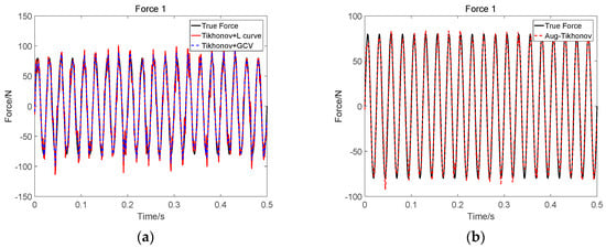
Figure 14. Identification result of two sinusoidal loads at SNR 40 dB (Force 1): (a) Tikhonov method; (b) the proposed method.

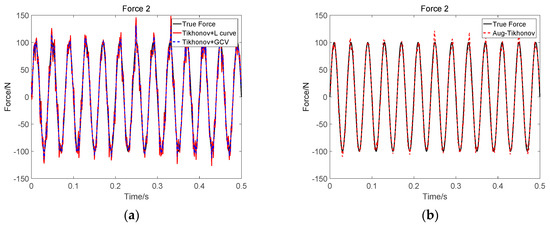
Figure 15. Identification result of two sinusoidal loads at SNR 40 dB (Force 2): (a) Tikhonov method; (b) the proposed method.

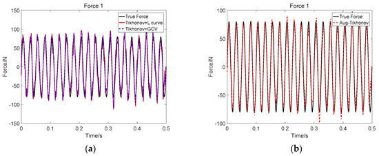
Figure 16. Identification result of two sinusoidal loads at SNR 30 dB (Force 1): (a) Tikhonov method; (b) the proposed method.

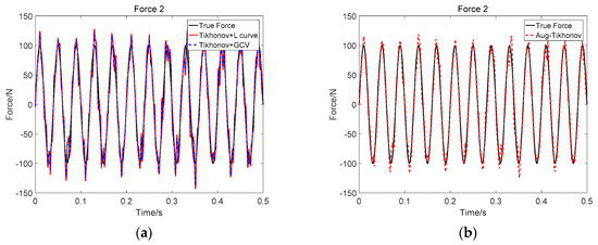
Figure 17. Identification result of two sinusoidal loads at SNR 30 dB (Force 2): (a) Tikhonov method; (b) the proposed method.

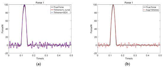
Figure 18. Identification result of two impact loads at SNR 40 dB (Force 1): (a) Tikhonov method; (b) the proposed method.

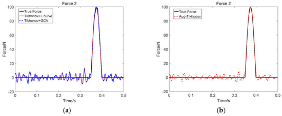
Figure 19. Identification result of two impact loads at SNR 40 dB (Force 2): (a) Tikhonov method; (b) the proposed method.

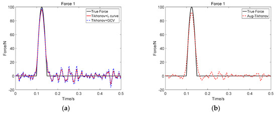
Figure 20. Identification result of two impact loads at SNR 30 dB (Force 1): (a) Tikhonov method; (b) the proposed method.

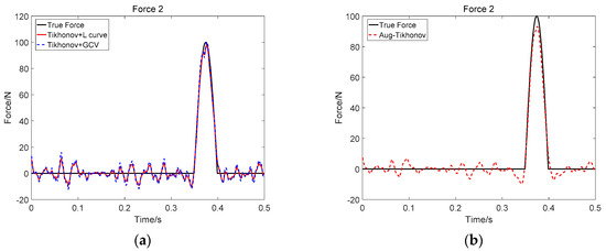
Figure 21. Identification result of two impact loads at SNR 30 dB (Force 2): (a) Tikhonov method; (b) the proposed method.

Table 2. Identification effect of two sinusoidal loads.

SNR	Force	Tikhonov + L Curve		Tikhonov + GCV		Augmented Tikhonov
		r	RE	r	RE	r	RE
40 dB	Force 1	96.91%	25.22%	98.69%	16.14%	99.38%	11.24%
	Force 2	97.81%	21.25%	99.06%	13.78%	99.55%	9.52%
30 dB	Force 1	96.33%	27.16%	97.03%	24.26%	98.21%	19.02%
	Force 2	97.02%	24.92%	97.65%	22.01%	98.72%	16.12%

Table 3. Identification effect of two impact loads.

SNR	Force	Tikhonov + L Curve		Tikhonov + GCV		Augmented Tikhonov
		r	RE	r	RE	r	RE
40 dB	Force 1	98.49%	16.75%	98.49%	16.75%	99.18%	12.29%
	Force 2	98.72%	15.39%	98.72%	15.39%	99.33%	11.11%
30 dB	Force 1	98.09%	18.65%	97.11%	22.98%	98.44%	17.30%
	Force 2	98.47%	16.80%	97.59%	21.19%	98.93%	15.46%

The results again confirm the previous set of conclusions. The accuracy of the augmented Tikhonov regularization method is consistently better than the Tikhonov regularization method. The augmented Tikhonov regularization method can effectively capture multiple loads for the four-degrees-of-freedom system. It should be noted that the identification accuracy is relatively lower when compared to a single load case. This is caused by the interaction in between the two loads. However, the identification results still capture all the dynamics of the external loads.

5.3. Single Force Identification on the Cantilever Beam

Next, to investigate the proposed augmented method for continuous system, we study the load identification on cantilever beam. The cantilever model is shown in Figure 22, and the parameters of the cantilever beam are: length $l=1\mathrm{m}$, cross-sectional area $A=0.0004{\mathrm{m}}^2$, moment of inertia $I=2.13\times {10}^{-9}{\mathrm{m}}^4$, Modulus of Elasticity $E=209\mathrm{Gpa}$, density $\rho =7800\mathrm{kg}/{\mathrm{m}}^3$, and Poisson’s ratio 0.3. The unknown load is applied at point 15, and the response is measured at point 17. Both points are displayed in Figure 22. Again, sinusoidal and impact loads are considered with the two previously considered noise levels, i.e., SNR = 30 and 40 dB. The system starts with a zero initial state. The time sampling interval is 1/1024 s, and the simulation time span is 1 s. For demonstration, the measured system response to the impulse load is shown in Figure 23. The identification results are listed in Figure 24, Figure 25, Figure 26 and Figure 27, and the accuracy of the load identification results are shown in Table 4.

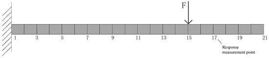
Figure 22. Cantilever model.

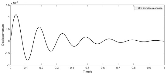
Figure 23. Unit impulse response diagram.

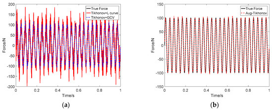
Figure 24. Identification result of sinusoidal load at SNR 40 dB on cantilever: (a) Tikhonov method; (b) the proposed method.

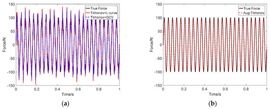
Figure 25. Identification result of sinusoidal load at SNR 30 dB on cantilever: (a) Tikhonov method; (b) the proposed method.

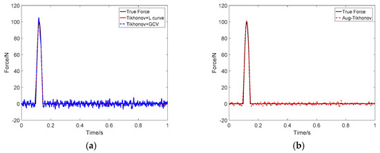
Figure 26. Identification result of impact load at SNR 40 dB on cantilever: (a) Tikhonov method; (b) the proposed method.

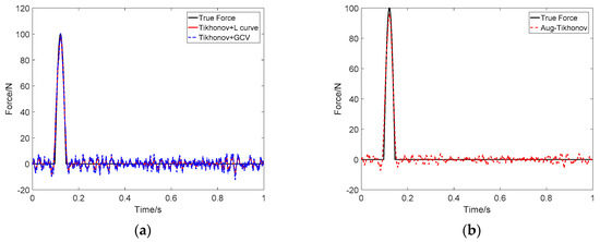
Figure 27. Identification result of impact load at SNR 30 dB on cantilever: (a) Tikhonov method; (b) the proposed method.

Table 4. Force identification effect of cantilever.

Force	SNR	Tikhonov + L Curve		Tikhonov + GCV		Augmented Tikhonov
		r	RE	r	RE	r	RE
sinusoidal load	40	69.91%	54.04%	68.05%	12.07%	99.72%	7.45%
	30	98.18%	26.81%	87.32%	20.40%	99.20%	12.66%
Impact load	40	97.49%	16.04%	96.26%	16.04%	99.44%	10.33%
	30	97.36%	16.67%	95.97%	21.91%	98.86%	14.83%

The results show that the proposed method can accurately identify the unknown loads on a continuous system, such as the considered cantilever beam. Consistent with the previous examples, the augmented Tikhonov method is more appropriate for solving the ill-posed problem of the load identification than the standard Tikhonov method. The sinusoidal load, under the two considered noise conditions, is identified with much better accuracy with the augmented method compared to the standard Tikhonov regularization method. The correlation coefficient and relative error of the results identified by tradition Tikhonov method are not as good as the proposed method, which suggests that the proposed method makes an improvement in the regularization parameters selected.

6. Experimental Examples

In this section, we aim to validate the proposed augmented method using experimental results. To this end, a load identification experiment for a simply supported bilateral beam is carried out. The model parameters are listed in Table 5. The natural frequency of the first four mode shapes are listed in Table 6. The frequencies are measured by modal experiment. To consider the model error and calculate the kernel function matrix, we build a finite element model and update it using the natural frequency obtained in the modal experiment. Table 6 shows the comparison of the natural frequency between the experimental results and the numerical results of the finite element model. The relative errors are evaluated based on the differences between the experimental and the numerical results. All the errors are smaller than 3%. Furthermore, for the first frequency, which is the most dominant, the error is less than 0.2%. These results verify that the finite element model is, in general, representative of the physical beam, and the numerical results are reliable. For demonstration, we show, in Figure 28, the displacements response obtained with the finite element model when an impulse load is applied.

Table 5. Parameter table of simply supported beam.

Parameters	Value
Length $a$	0.7 m
Width $b$	0.04 m
Thickness $h$	0.008 m
Density $\rho$	7800 kg/m3
Elastic Modulus $E$	209 GPa
Poisson’s ratio $\mu$	0.30

Table 6. The comparison of natural frequencies of the beam.

Mode	Experimental Natural Frequency (Hz)	Simulation Natural Frequency (Hz)	Relative Error (%)
1	38.13	38.07	0.15
2	150.35	152.19	1.22
3	334.63	341.93	2.18
4	593.00	605.92	2.18

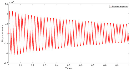
Figure 28. The impulse response diagram of the simply supported beam.

Figure 29 shows the experimental setting of the considered beam, while, in Table 7, we specify the used instruments. To apply a load on the beam, the exciter is installed at 0.42 m from one end. The force sensor is installed on the exciter connecting rod to measure the actual applied load. The laser displacement sensor is installed at 0.28 m from the beam end to measure the displacement response. A sampling rate of 4096 is used. Two different loads are applied. First, a sinusoidal and then a triangle wave signal is applied using the exciter. The load magnitude is adjusted through a power amplifier. The load applied is then recovered using the proposed method and the measured displacement. The identified load is compared to the actual load measured as by the force sensor.

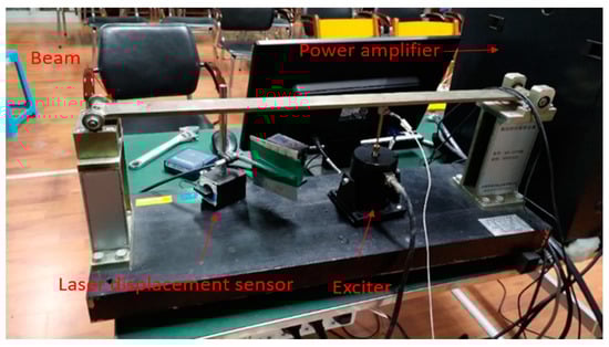
Figure 29. The load identification experiment site.

Table 7. Force identification experiment equipment.

Equipment	Name
Excitation	JZT-2 Permanent magnet exciter
Power amplifier	HEAS-50 Power amplifier
Dynamic signal acquisition board	NI PXIe-4499 Capture card
Signal acquisition instrument	NI PXI
Sensor	optoNCDT2300 Laser displacement sensor
Software	NI Signal Express

Figure 30 shows the measured displacement response of the sinusoidal, as well as the triangular, loads. Using the proposed augmented Tikhonov regularization method, ${\beta }_2$ selection results are shown in Figure 31. The load identification results are shown in Figure 32 and Figure 33, respectively. The results accuracy is evaluated in Table 8.

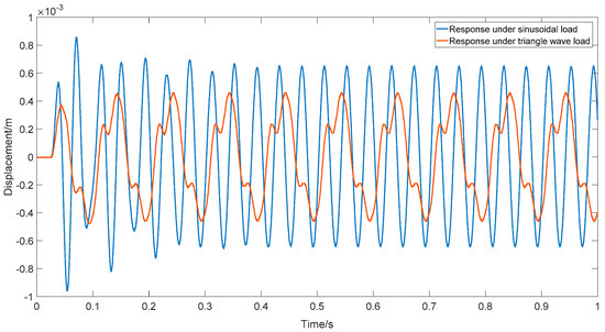
Figure 30. The displacement response.

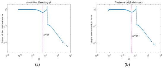
Figure 31. ${\beta }_2$ ignition value selection: (a) sinusoidal load; (b) triangle wave load.

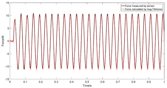
Figure 32. Identification result of sinusoidal load.

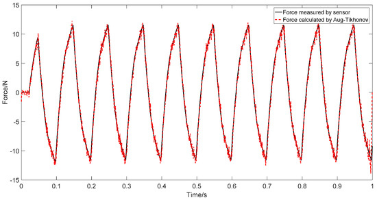
Figure 33. Identification result of triangle wave load.

Table 8. Evaluation of identification results of experiment.

Force	Correlation Coefficient (r)	Relative Error (RE)
Sinusoidal load	99.42%	8.07%
Triangle wave load	99.55%	9.83%

The results in this section show experimentally that the proposed method can accurately identify the external loads applied on the considered beam. Figure 29 shows that the sinusoidal load is accurately recovered. Both the actual load period and amplitude match those obtained with the proposed approach with high accuracy. The zero initial stage and the initial change in the load amplitude for the first few cycles are all accurately reflected in the load identification. A similar observation can also be made for the triangular wave load identification. The load period, amplitude, and initial changes are all recovered with good accuracy, as can be seen in Figure 30. The correlation coefficients, for both types of considered loads, are above 99%. Similarly, the relative error is around 10% for both loads.

7. Conclusions

In this paper, we proposed the augmented Tikhonov regularization method in combination with the Green kernel function to identify the external dynamic loads acting on a structure. We also proposed a method for the initial values selection of the regularization parameters. An iterative algorithm for the load identification process was presented. The algorithm performance was evaluated using numerical, as well as experimental, studies. First, we used three numerical examples. The examples showed the efficiency and accuracy of the proposed method for different types of loading, including: an impact load, a sinusoidal wave, or a triangle wave load. The comparisons in these examples show that the proposed method outperforms the standard Tikhonov regularization method for load identification, even when considering noise in the input data. Moreover, the proposed method shows better stability than the standard method, which is attributed to the selection of the regularization parameters. After the numerical examples, we performed an experimental study to further validate the augmented method in a practical application. The method shows high accuracy in capturing different type of loading despite the inaccuracies in the measurement, as well as in the model, parameters. Dynamic load identification, in real conditions, is often affected by constant noise levels, which inevitably appear in the identification results. In the standard Tikhonov method, the noise can result in large fluctuations in the identified load. This is mitigated in the augmented Tikhonov method by a proposed approach to identify the initial parameters based on the noise characteristics. If the noise level does not change, the identification results are stable. Moreover, the paper also proposes a parameters selection approach where the noise level is unknown. Here, the initial parameter ${\beta }_1$ was chosen to be close to zero, while ${\beta }_2$ was chosen based on the slope of the residual norm $\left|\right|Hf-y{\left|\right|}_2^2$. Using this selection process, the values of ${\beta }_1$ and ${\beta }_2$ were chosen without knowing the noise level; hence, the process can be of great significance in practical engineering application. Moreover, the regularization parameters selected by the L-curve and GCV methods are not always optimal, which can lead to large errors. This is especially the case when the input data is noisy. However, the results show that the regularization parameters, selected by the proposed method, can still lead to accurate results even with relatively high level of noise.

This paper presents a first attempt to utilize an augmented Tikhonov regularization method combined with the Green kernel function for load identification. Such a problem can be especially challenging due to the fact that they often are ill-posed. The proposed method to identify dynamic load can have a wide range of applications in several domains, such as design optimization, diagnostics, control, and monitoring of vibrating structures.

References

- Wang, L.; Huang, Y.; Xie, Y.; Du, Y. A new regularization method for dynamic load identification. Sci. Prog. 2020, 103, 0036850420931283. [Google Scholar] [CrossRef] [PubMed]
- He, Z.C.; Zhang, Z.; Li, E. Random dynamic load identification for stochastic structural-acoustic system using an adaptive regularization parameter and evidence theory. J. Sound Vib. 2020, 471, 115188. [Google Scholar] [CrossRef]
- Wang, L.; Liu, J.; Xie, Y.; Gu, Y. A new regularization method for the dynamic load identification of stochastic structures. Comput. Math. Appl. 2018, 76, 741–759. [Google Scholar] [CrossRef]
- Li, X.; Zhao, H. Force Identification Based on Measuring Point Selection and Improved L-Curve Method. J. Shanghai Jiaotong Univ. 2020, 54, 569–576. [Google Scholar]
- Lu, G. Vibration transfer path analysis of rocket engine based on weighted regularization. J. Vib. Shock 2019, 38, 271–276. [Google Scholar]
- Li, J. Identification of Longitudinal Load of Propeller-Shaft-Boat System Based on Regularization Technology and Subspace Method; Huazhong University of Science and Technology: Wuhan, China, 2019. [Google Scholar]
- Wang, N.; Ren, C. Novel fractional order Tikhonov regularization load reconstruction technique and its application. J. Vib. Shock 2019, 38, 121–126, 158. [Google Scholar]
- Miu, B.; Zhou, F. Research of the structure load identification hybrid technology using kernel function and different regularization method. J. Vib. Eng. 2018, 31, 553–560. [Google Scholar]
- Boukria, Z.; Perrotin, P.; Bennani, A. Experimental impact force location and identification using inverse problems: Application for a circular plate. Int. J. Mech. 2011, 5, 48–55. [Google Scholar]
- Thite, A.N.; Thompson, D.J. The quantification of structure-borne transmission paths by inverse methods. Part 1: Improved singular value rejection methods. J. Sound Vib. 2003, 264, 411–431. [Google Scholar] [CrossRef]
- Choi, H.G.; Thite, A.N.; Thompson, D.J. Comparison of methods for parameter selection in Tikhonov regularization with application to inverse force determination. J. Sound Vib. 2007, 304, 894–917. [Google Scholar] [CrossRef]
- Ma, C.; Hua, H. State space load identification technique based on an improved regularized method. J. Vib. Shock 2015, 34, 146–149. [Google Scholar]
- Gao, W. Research on Dynamic Load Identification Method and Application Based on Regularization; Harbin Institute of Technology: Harbin, China, 2016. [Google Scholar]
- Qiao, B.; Zhang, X.; Wang, C.; Zhang, H.; Chen, X. Sparse regularization for force identification using dictionaries. J. Sound Vib. 2016, 368, 71–86. [Google Scholar] [CrossRef]
- Zhou, S. Research and Application of Load Reverse Method Based on Tikhonov Regularization Technology; Hu’nan University: Changsha, China, 2016. [Google Scholar]
- Isakov, V. Inverse problems for partial differential equations. Appl. Math. Sci. 1979, 703, 93–98. [Google Scholar]
- Jin, B.; Zou, J. A Bayesian inference approach to the ill-posed Cauchy problem of steady-state heat conduction. Int. J. Numer. Methods Eng. 2008, 76, 521–544. [Google Scholar] [CrossRef]
- He, Y. A Bayesian Regularization-based Method for Identification of Impact Force on Composite Structure; Nanjing University of Aeronautics and Astronautics: Nanjing, China, 2018. [Google Scholar]
- Jin, B.; Zou, J. Augmented Tikhonov regularization. Inverse Probl. 2009, 25, 025001. [Google Scholar] [CrossRef]
- Lei, B.; Zheng, H. Dynamic Load Identification Approach Based on Bayesian Estimation. Noise Vib. Control. 2018, 38, 215–219. [Google Scholar]
- Aucejo, M.; De Smet, O. An optimal Bayesian regularization for force reconstruction problems. Mech. Syst. Signal Process. 2019, 126, 98–115. [Google Scholar] [CrossRef]
- Li, Q.; Lu, Q. A revised time domain force identification method based on Bayesian formulation. Int. J. Numer. Methods Eng. 2019, 118, 411–431. [Google Scholar] [CrossRef]
- Sun, Y.; Luo, L.; Chen, K.; Qin, X.; Zhang, Q. A time-domain method for load identification using moving weighted least square technique. Comput. Struct. 2020, 234, 106254. [Google Scholar] [CrossRef]
© 2020 by the authors. Licensee MDPI, Basel, Switzerland. This article is an open access article distributed under the terms and conditions of the Creative Commons Attribution (CC BY) license (http://creativecommons.org/licenses/by/4.0/).