An Improved Grey Wolf Optimizer Based on Differential Evolution and OTSU Algorithm

Abstract

Aimed at solving the problems of poor stability and easily falling into the local optimal solution in the grey wolf optimizer (GWO) algorithm, an improved GWO algorithm based on the differential evolution (DE) algorithm and the OTSU algorithm is proposed (DE-OTSU-GWO). The multithreshold OTSU, Tsallis entropy, and DE algorithm are combined with the GWO algorithm. The multithreshold OTSU algorithm is used to calculate the fitness of the initial population. The population is updated using the GWO algorithm and the DE algorithm through the Tsallis entropy algorithm for crossover steps. Multithreshold OTSU calculates the fitness in the initial population and makes the initial stage basically stable. Tsallis entropy calculates the fitness quickly. The DE algorithm can solve the local optimal solution of GWO. The performance of the DE-OTSU-GWO algorithm was tested using a CEC2005 benchmark function (23 test functions). Compared with existing particle swarm optimizer (PSO) and GWO algorithms, the experimental results showed that the DE-OTSU-GWO algorithm is more stable and accurate in solving functions. In addition, compared with other algorithms, a convergence behavior analysis proved the high quality of the DE-OTSU-GWO algorithm. In the results of classical agricultural image recognition problems, compared with GWO, PSO, DE-GWO, and 2D-OTSU-FA, the DE-OTSU-GWO algorithm had accuracy in straw image recognition and is applicable to practical problems. The OTSU algorithm improves the accuracy of the overall algorithm while increasing the running time. After adding the DE algorithm, the time complexity will increase, but the solution time can be shortened. Compared with GWO, DE-GWO, PSO, and 2D-OTSU-FA, the DE-OTSU-GWO algorithm has better results in segmentation assessment.

1. Introduction

Image segmentation is an important part of image processing in practice [1,2,3,4,5], as well as a key image analysis technique [6,7,8,9,10]. The threshold image segmentation method divides pixels into several classes by setting the threshold value to realize the separation of the object and the background in the image. Threshold segmentation based on a histogram is the most widely used image segmentation method. The histogram is used for analysis. A better threshold is selected according to the relationship between the peaks and troughs of the histogram [11,12,13].

Shannon, Otsu, and Kapur are the most common methods. Shannon entropy is used to determine the amount of information contained in a random data source [14]. The OTSU algorithm is an automatic method to determine the threshold using the maximum interclass variance [15]. Kapur entropy is the pixel grey value with the maximum entropy of the whole image [16]. Two-dimensional OTSU algorithm by Liu and Li integrates the average grey value of neighborhood pixels on the basis of one-dimensional OTSU [17].

Heuristic algorithm is proposed relative to the optimization algorithm, in which genetic algorithm (GA) [18], particle swarm optimizer (PSO) [19], and grey wolf optimizer algorithm (GWO) [20] are applied in various research fields.

Zahara et al. proposed a hybrid optimization scheme for multiple thresholding by the criteria of OTSU, Gaussian function, and PSO algorithms [21]. Cui et al. proposed a threshold segmentation algorithm based on 2D grey histogram and PSO for fire image segmentation [22]. An improved two-dimensional OTSU algorithm based on PSO was proposed to find the optimal threshold for lung parenchyma segmentation and extraction by Helen et al. [23]. The multithresholding based on modified PSO (MMPSO) method by Hamdaoui et al. was a PSO algorithm based on the new fitness function and OTSU method or multilevel thresholding [24]. Khairuzzaman et al. used Kapur entropy and OTSU combined with GWO algorithm to apply the multithreshold problem [25]. Ibrahim et al. proposed a multilevel threshold optimization method based on GWO. These principles included chaotic logistic map, the opposition-based learning (OBL), differential evolution (DE) algorithm, and the disruption operator (DO) [26]. Bohat et al. proposed the WOA-TH, GWO-TH, and PSO TH algorithm [27]. Zhou et al. proposed a method combining two-dimensional OTSU image threshold segmentation and improved firefly algorithm [28].

This paper proposes an improved GWO algorithm. There is an improved GWO algorithm for initial population selection and threshold selection. By combining the GWO algorithm with the three principles, multithreshold OTSU, Tsallis entropy, and differential evolution (DE) algorithms, an improved GWO algorithm based on the DE algorithm and the OTSU algorithm is proposed (DE-OTSU-GWO). Each principle has its own function. Multithreshold OTSU calculates the fitness in the initial population and makes the initial stage basically stable. Tsallis entropy quickly calculates the fitness. Differential evolution can solve the local optimal solution of the GWO algorithm.

Compared with existing PSO and GWO algorithms, the experimental results show the stability, accuracy, and convergence of the DE-OTSU-GWO algorithm. In addition, when compared with other algorithms, a convergence behavior analysis proves the high quality of the DE-OTSU-GWO algorithm.

The rest of the paper is organized as follows. Section 2 describes an improved GWO based on the DE and OTSU algorithms. Section 3 presents the experimental results and analysis. Section 4 details an experiment and discusses the best method for straw coverage detection. The last section summarizes this article.

2. Materials and Methods

2.1. Multithreshold OTSU

The original OTSU method is a better threshold selection algorithm in image segmentation. This method is simple and is not affected by the brightness and contrast of the image. However, the original OTSU method is a single-threshold segmentation method. After using the algorithm to divide the image into two classes, the target within the two classes can no longer be distinguished. It is possible to distinguish other targets between the two classes; therefore, we need to further divide these two classes. The multithreshold OTSU method is used to segment different classes. Assuming there are m classes to be distinguished in an image X, there are m − 1 thresholds $k_1,\cdots ,k_n,\cdots ,k_{m-1}$, which are used to divide image X into m classes. These classes are represented as $C_0=\left\{0,1,\cdots ,k_1\right\},\cdots ,C_n=\left\{k_n+1,k_n+2,\cdots ,k_{n+1}\right\},\cdots ,C_m=\left\{k_m+1,k_m+2,\cdots ,L-1\right\}$. The interclass variance [29,30] is as follows. (The use of the formula symbol in this section is shown in

Table 1. The implication of the formula symbol in Section 2.

Symbol	Implication	Symbol	Implication
$\mathrm{N}$	total number of pixels in the greyscale image	$r1, r2, \mathrm{and} r3$	mutually different random integers chosen from 1 to N
$n$	the number of pixels in the same greyscale pixel $i$.	$randb\left(j\right)$	random value, ∈ [ 0,1 ]
${\omega }_i$	the probability of the same greyscale pixel	$CR$	crossover constant, $\in \left[ 0,1 \right]$
$\mu$	the pixel mean	$rnbr\left(i\right)$	a randomly chosen index
$q$	selected by using the histogram mean value of the segmentation image.	$D$	determines $z_i\left(t+1\right)$ has at least one parameter from the target individual $y_i\left(t+1\right)$
$V$	threshold	$\overrightarrow{D}$	the distance between the wolves and the optimal threshold
$d$	the grey level in the range of 0~99	$t$	current iteration
$m$	the grey level in the range of 100~149	$\overrightarrow{A}$ and $\overrightarrow{C}$	coefficient vectors
$l$	the grey level in the range of 150~255	$\overrightarrow{X_P}$	the position vector of the prey
$y$	mutant vector	$\overrightarrow{X}$	the position vector of the wolf
$x$	target vector	$\overrightarrow{a}$	linearly decreased from 2 to 0 over the course of iterations
$F$	F∈ [ 0,2 ], real and constant factor controls the amplification of the differential variation $(x_{r2}\left(t\right)-x_{r3}\left(t\right)$.	$\overrightarrow{r_1}$ and $\overrightarrow{r_2}$	random vectors in [ 0,1 ]

).

$$\mathsf{\sigma }={\omega }_0{\left({\mu }_0-{\mu }_T\right)}^2+\cdots +{\omega }_n{\left({\mu }_n-{\mu }_T\right)}^2+\cdots +{\omega }_{m-1}{\left({\mu }_{m-1}-{\mu }_T\right)}^2$$

(1)

$${\omega }_0={\displaystyle \sum }_{i=0}^{k_i}{P}_i,\cdots ,{\omega }_n={\displaystyle \sum }_{i=k_n+1}^{k_{n+1}}{P}_i,\cdots ,{\omega }_{m-1}={\displaystyle \sum }_{i=k_{m-1}+1}^{L-1}{P}_i$$

(2)

$${\mu }_0=\frac{{\sum }_{i=0}^{k_i}i{P}_i}{{\omega }_0},\cdots ,{\mu }_n=\frac{{\sum }_{i=k_n+1}^{k_{n+1}}i{P}_i}{{\omega }_n},\cdots ,{\mu }_0=\frac{{\sum }_{i=k_{m-1}+1}^{L-1}i{P}_i}{{\omega }_{m-1}}$$

(3)

$$\mathrm{N}={\displaystyle \sum }_{i=0}^{L-1}{N}_i$$

(4)

$${\mu }_T={\displaystyle \sum }_{i=0}^{L-1}i{P}_i$$

(5)

A set of thresholds that maximize the ${\mathsf{\sigma }}_{BC}$ is the desired threshold.

2.2. Tsallis Entropy

An entropy criterion is selected to determine the threshold in threshold segmentation. Compared with Shannon entropy threshold segmentation, Tsallis entropy can be extended to nongeneralized systems.

For an image with G grey levels, $p_i$ is the probability of the greyscale i appearing in the image. Tsallis entropy $S_q$ for each distribution is as follows:

$$S_q=\frac{1-{\sum }_{i=1}^k{\left(p_i\right)}^q}{q-1}$$

(6)

In the case of single-threshold segmentation, let threshold $z$ divide the image into two classes: target part A and background part B. The grey probability of these two parts is as follows:

$$\{\begin{array}{c}{w}_A={\displaystyle {\displaystyle \sum }_{i=1}^z}{p}_i\\ w_B={\displaystyle {\displaystyle \sum }_{i=z+1}^{G-1}}{p}_i\end{array}$$

(7)

$$w_A+w_B=1$$

(8)

Tsallis entropy of two parts is as follows:

$$S_q^A\left(t\right)=\frac{\left[1-{\sum }_{i=1}^z{\left(\frac{p_i}{w_A}\right)}^q\right]}{q-1}$$

(9)

$$S_q^B\left(t\right)=\frac{\left[1-{\sum }_{i=z+1}^{G-1}{\left(\frac{p_i}{w_B}\right)}^q\right]}{q-1}$$

(10)

The total Tsallis entropy is as follows:

$${\mathrm{S}}_q^{A+B}\left(z\right)=S_q^A\left(z\right)+S_q^B\left(z\right)+\left(1-q\right)S_q^A\left(z\right)S_q^B\left(z\right)$$

(11)

Set $E_1=\sum _{i=0}^t{(\frac{p_i}{w_1})}^q$, and extend it from a single threshold to multilevel thresholds with thresholds $R$. Tsallis entropy $S_q\left(\left[t_1,t_2\cdots t_R\right]\right)$ [31] is as follows:

$$S_q\left(\left[t_1,t_2\cdots t_R\right]\right)=\frac{1}{1-q}{E}_1{E}_2\cdots E_{R-1}$$

(12)

$$q=\{\begin{array}{cc}0.05+{0.5}^V & G\in l\\ 0.15+{0.5}^V & G\in m\\ 0.01+0.2\times \left|V-2\right|/V& G\in d\end{array}$$

(13)

2.3. Differential Evolution

Differential evolution (DE) algorithm is a global optimal random search based on population iteration. Like the other genetic algorithms (GAs), DE algorithm begins with an initial population vector containing many target individuals. The current generation evolves through a repeating evolutionary process to the next generation until the termination condition is reached. DE algorithm includes mutation, crossover, and selection operations [32].

The mutation operation generates a new parameter vector by adding the weighted difference between two population vectors to a third vector, as follows:

$$y_i\left(t+1\right)=x_{r1}\left(t\right)+F·\left(x_{r2}\left(t\right)-x_{r3}\left(t\right)\right)$$

(14)

The crossover operation increases the diversity of the perturbed parameter vectors. The trial vector is as follows:

$$z_i\left(t+1\right)=\left(z_{1i}\left(t+1\right),z_{2i}\left(t+1\right),\cdots ,z_{Di}\left(t+1\right)\right)$$

(15)

The crossover operation is as follows:

$$z_{ji}\left(t+1\right)=\{\begin{array}{c}{y}_{ji}, if\left(randb\left(j\right)\le CR\right) or j=rnbr\left(i\right)\\ x_{ji}, if\left(randb\left(j\right)>CR\right) and j\ne rnbr\left(i\right)\end{array}$$

(16)

$$j=1,2,\cdots ,D$$

(17)

The selection operation is compared to the target vector using the greedy criterion, as follows:

$$x_i\left(t+1\right)=\{\begin{array}{c}{z}_i\left(t+1\right), f\left[z_i\left(t+1\right)\right]<f\left[x\left(t\right)\right]\\ x\left(t\right), f\left[z_i\left(t+1\right)\left]\ge f\right[x\left(t\right)\right]\end{array}$$

(18)

2.4. Grey Wolf Optimizer

The grey wolf optimizer (GWO) algorithm simulates the hierarchy and hunting behavior of grey wolves. Grey wolves have a very strict social dominance hierarchy:

Alpha (α) is the leader and is the best in terms of managing the pack; however, it is not the strongest member of the pack. This suggests that organization and discipline are more important than strength.

Beta (β) obeys alpha and can command other lower-level wolves. In addition, beta transmits alpha commands and provides feedback to alpha.

Delta (δ) obeys alpha and beta. Omega rules over his inferiors.

Omega (ω) is balanced within the population and is subject to all other dominant wolves.

The main stages of grey wolf hunting are as follows: encircling, hunting, and attacking. The behavior process of encircling prey is as follows:

$$\overrightarrow{D}=\left|\overrightarrow{C}·\overrightarrow{X_P}\left(t\right)-\overrightarrow{X}\left(t\right)\right|$$

(19)

$$\overrightarrow{X}\left(t+1\right)=\overrightarrow{X_P}\left(t\right)-\overrightarrow{A}·\overrightarrow{D}$$

(20)

$$\overrightarrow{A}=2\overrightarrow{a}·\overrightarrow{r_1}-\overrightarrow{a}$$

(21)

$$\overrightarrow{C}=2·\overrightarrow{r_2}$$

(22)

The hunting process is usually guided by alpha. Beta and delta might occasionally participate in hunting. According to the best search agent location, other search agents (including omega) should update their positions. Note the following formulas:

$$\{\begin{array}{c}\overrightarrow{D_{\alpha }}=\left|\overrightarrow{C_1}\cdot \overrightarrow{X_{\alpha }}\right|\\ \overrightarrow{D_{\beta }}=\left|\overrightarrow{C_2}\cdot \overrightarrow{X_{\beta }}\right|\\ \overrightarrow{D_{\delta }}=\left|\overrightarrow{C_3}\cdot \overrightarrow{X_{\delta }}\right|\end{array}$$

(23)

$$\{\begin{array}{c}\overrightarrow{X_1}=\overrightarrow{X_{\alpha }}-\overrightarrow{A_1}\cdot \left(\overrightarrow{D_{\alpha }}\right)\\ \overrightarrow{X_2}=\overrightarrow{X_{\beta }}-\overrightarrow{A_2}\cdot \left(\overrightarrow{D_{\beta }}\right)\\ \overrightarrow{X_3}=\overrightarrow{X_{\delta }}-\overrightarrow{A_3}\cdot \left(\overrightarrow{D_{\delta }}\right)\end{array}$$

(24)

$$\overrightarrow{X}\left(t+1\right)=\left(\overrightarrow{X_1}+\overrightarrow{X_2}+\overrightarrow{X_3}\right)/3$$

(25)

The attacking is the final stage. When the prey stops moving, the grey wolves attack to end the hunting process. The GWO algorithm obtains the optimal threshold. The process model building is mainly realized by the decreasing of value $\overrightarrow{a}$ [20].

However, the threshold value may fall into the local optimal solution with the operators after the GWO algorithm finishes the iteration.

2.5. The Proposed Method

A flowchart of the proposed algorithm is shown in Figure 1. The pseudo-code of the proposed algorithm is shown in Figure 2. The multithreshold OTSU algorithm is used to calculate the fitness of the initial population. The population is updated using the GWO algorithm and the DE algorithm through the Tsallis entropy algorithm for crossover steps. The OTSU algorithm is stable and not affected by the image brightness and contrast. The Tsallis entropy algorithm can increase the flexibility and adaptability of the algorithm. The DE algorithm prevents the threshold of the GWO algorithm from falling into the local optimal solution. GWO is used as a global search method with good search domain detection capabilities. Each stage of the proposed algorithm is described in detail below.

2.5.1. Initial Stage

After initializing the grey wolf population X and defining the parameters, calculate the fitness of each search agent by the multithreshold OTSU algorithm.

If there are m classes to be distinguished in wolves $X=0,1,\cdots ,L-1$, then there are m − 1 thresholds.$k_1,\cdots ,k_j,\cdots ,k_{m-1}$ is used to classify X into m groups of wolves. The variance between classes is as follows:

$$\mathsf{\sigma }={\displaystyle \sum }_{i=0}^M{\omega }_i{\left({\mu }_{\mathrm{i}}-{\mu }_T\right)}^2$$

(26)

$${\omega }_j={\displaystyle \sum }_{i=k_j+1}^{k_{\mathrm{j}+1}}\frac{n_i}{N}$$

(27)

$${\mu }_j=\frac{{{\displaystyle \sum }}_{i=k_j+1}^{k_{j+1}}i{P}_i}{{\omega }_j}$$

(28)

$$\mathrm{N}={\displaystyle \sum }_{i=0}^{L-1}{N}_i;{\mu }_T={\displaystyle \sum }_{i=0}^{L-1}i{P}_i={\displaystyle \sum }_{j=0}^m{\omega }_j{\mu }_j={\displaystyle \sum }_{j=0}^m{\omega }_j$$

(29)

The fitness of wolves, namely, the threshold value $X_1,X_2,\cdots ,X_{\mathrm{n}}$, is as follows:

$$\{\begin{array}{c}{X}_1=\frac{{\mu }_0+{\mu }_1}{2}\\ X_2=\frac{{\mu }_1+{\mu }_2}{2}\\ \cdots \\ X_{\mathrm{n}}=\frac{{\mu }_{\mathrm{n}-1}+{\mu }_{\mathrm{n}}}{2}\end{array}$$

(30)

The multithreshold OTSU algorithm improves the selection of fitness screening, and the overall fitness becomes more accurate and stable.

2.5.2. Updating Stage

This stage is used to update the fitness and $\overrightarrow{X_{\alpha }}, \overrightarrow{X_{\beta }}, and \overrightarrow{X_{\delta }}$ position for the next stage.

2.5.3. Calculating Stage

In this stage, the solutions are updated in two steps. In the first step, the GWO algorithm and DE algorithm are computed separately. In the second step, the crossover and selection are used. These two steps are discussed in detail below.

The distance $\overrightarrow{D_{\alpha }}, \overrightarrow{D_{\beta }}, and \overrightarrow{D_{\delta }}$ between the wolves and the optimal threshold is calculated though the GWO algorithm. The position vectors of the wolf $\overrightarrow{X_{\alpha }}, \overrightarrow{X_{\beta }}, and \overrightarrow{X_{\delta }}$ are determined. Next, the position vector $\overrightarrow{X}$ is updated.

The mutation population $y_i\left(t+1\right)$ is generated by a mutation operation of the DE algorithm.

2.5.4. Crossing and Selecting Stages

According to the mutation population obtained, all search agents perform crossover operation. Next, produce a new search agent that combines the GWO algorithm and DE algorithm. Then, select the better item from the fitness of the updating stage and the fitness of this stage that the new search agent produced.

3. Results and Discussion

In this section, we use a set of unconstrained benchmark functions. There are 23 benchmark functions (7 groups of unimodal benchmark functions, 6 groups of multipeak benchmark functions, and 10 groups of fixed-dimension multipeak benchmark functions) in CEC 2005 test functions [33]. These test functions were selected to compare our results with those of the current meta-heuristic. The test functions will replace the algorithm that calculates fitness. These benchmark functions are shown in

Table 2. Unimodal benchmark functions.

Function	Dim	Range	${\mathit{f}}_{\mathit{m}\mathit{i}\mathit{n}}$
$f_1\left(x\right)={\displaystyle {\displaystyle \sum }_{i=1}^n}{x}_i^2$	30	[ −100, 100 ]	0
$f_2\left(x\right)={\displaystyle {\displaystyle \sum }_{i=1}^n}\left|x_i\right|+{\displaystyle {\displaystyle \prod }_{i=1}^n}\left|x_i\right|$	30	[ −10, 10 ]	0
$f_3\left(x\right)={\displaystyle {\displaystyle \sum }_{i=1}^n}{\left({\displaystyle {\displaystyle \sum }_{j-1}^i}{x}_j\right)}^2$	30	[ −100, 100 ]	0
$f_4\left(x\right)=ma{x}_i\left\{\left|x_i\right|,1\le i\le n\right\}$	30	[ −100, 100 ]	0
$f_5\left(x\right)={\displaystyle {\displaystyle \sum }_{i=1}^{n-1}}\left[100{\left(x_{i+1}-x_i^2\right)}^2+{\left(x_i-1\right)}^2\right]$	30	[ −30, 30 ]	0
$f_6\left(x\right)={\displaystyle {\displaystyle \sum }_{i=1}^n}{\left(\left[x_i+0.5\right]\right)}^2$	30	[ −100, 100 ]	0
$f_7\left(x\right)={\displaystyle {\displaystyle \sum }_{i=1}^n}i{x}_i^4+random\left[0,1\right)$	30	[ −1.28, 1.28 ]	0

,

Table 3. Multimodal benchmark functions.

Function	Dim	Range	${\mathit{f}}_{\mathit{m}\mathit{i}\mathit{n}}$
$f_8\left(x\right)={\displaystyle {\displaystyle \sum }_{i=1}^n}-x_{i}sin\left(\sqrt{\left|x_i\right|}\right)$	30	[ −500, 500 ]	−418.9829 × 5
$f_9\left(x\right)={\displaystyle {\displaystyle \sum }_{i=1}^n}\left[x_i^2-10cos\left(2\pi x_i\right)+10\right]$	30	[ −5.12, 5.12 ]	0
$f_{10}\left(x\right)=-20exp\left(-0.2\sqrt{\frac{1}{n}{\displaystyle {\displaystyle \sum }_{i=1}^n}{x}_i^2}\right)-exp\left(\frac{1}{n}{\displaystyle {\displaystyle \sum }_{i=1}^n}\cos \left(2\pi x_i\right)\right)+20+e$	30	[ −32, 32 ]	0
$f_{11}\left(x\right)=\frac{1}{4000}{\displaystyle {\displaystyle \sum }_{i=1}^n}{x}_i^2-{\displaystyle {\displaystyle \prod }_{i=1}^n}\cos \left(\frac{x_i}{\sqrt{i}}\right)+1$	30	[ −600, 600 ]	0
$f_{12}\left(x\right)=\frac{\pi }{n}\left\{10sin\left(\pi y_1\right)+{\displaystyle {\displaystyle \sum }_{i=1}^{n-1}}{\left(y_i-1\right)}^2\left[1+10si{n}^2\left(\pi y_{i+1}\right)\right]+{\left(y_n-1\right)}^2\right\}+{\displaystyle {\displaystyle \sum }_{i=1}^n}u\left(x_i,10,100,4\right)$ $y_i=1+\frac{x_i+1}{4}$ $u\left(x_i,a,k,m\right)=\{\begin{array}{c}k{\left(x_i-a\right)}^m x_i>a\\ 0 -a<x_i<a\\ k{\left(-x_i-a\right)}^m x_i<-a\end{array}$	30	[ −50, 50 ]	0
$f_{13}\left(x\right)=0.1\left\{si{n}^2\left(3\pi x_1\right)+{\displaystyle {\displaystyle \sum }_{i=1}^n}{\left(x_i-1\right)}^2\left[1+si{n}^2\left(3\pi x_i+1\right)\right]+{\left(x_n-1\right)}^2\left[1+si{n}^2\left(2\pi x_n\right)\right]\right\}+{\displaystyle {\displaystyle \sum }_{i=1}^n}u\left(x_i,5,100,4\right)$	30	[ −50, 50 ]	0

and

Table 4. Fixed-dimension multimodal benchmark functions.

Function	Dim	Range	${\mathit{f}}_{\mathit{m}\mathit{i}\mathit{n}}$
$f_{14}\left(x\right)={\left(\frac{1}{500}+{\displaystyle {\displaystyle \sum }_{j=1}^{25}}\frac{1}{j+{{\displaystyle \sum }}_{i=1}^2{\left(x_i-a_{ij}\right)}^6}\right)}^{-1}$	2	[ −65.536, 65.536 ]	1
$f_{15}\left(x\right)={\displaystyle {\displaystyle \sum }_{i=1}^{11}}{\left[a_i-\frac{x_1\left(b_i^2+b_i{x}_2\right)}{b_i^2+b_i{x}_3+x_4}\right]}^2$	4	[ −5, 5 ]	0.00030
$f_{16}\left(x\right)=4x_1^2-2.1x_1^4+\frac{1}{3}{x}_1^6+x_1{x}_2-4x_2^2+4x_2^4$	2	[ −5, 5 ]	−1.0316
$f_{17}\left(x\right)={\left(x_2-\frac{5.1}{4{\pi }^2}{x}_1^2+\frac{5}{\pi }{x}_1-6\right)}^2+10\left(1-\frac{1}{8\pi }\right)cos{x}_1+10$	2	[ −5, 5 ]	0.398
$f_{18}\left(x\right)=\left[1+{\left(x_1+x_2+1\right)}^2\left(19-14x_1+3x_1^2-14x_2+6x_1{x}_2+3x_2^2\right)\right]\times \left[30+{\left(2x_1-3x_2\right)}^2\times \left(18-32x_1+12x_1^2+48x_2-36x_1{x}_2+27x_2^2\right)\right]$	2	[ −2, 2 ]	3
$f_{19}\left(x\right)=-{\displaystyle {\displaystyle \sum }_{i=1}^4}{c}_{i}exp(-{\displaystyle {\displaystyle \sum }_{j=1}^3}{a}_{ij}{\left(x_j-p_{ij}\right)}^2$	3	[ 1, 3 ]	−3.86
$f_{20}\left(x\right)=-{\displaystyle {\displaystyle \sum }_{i=1}^4}{c}_{i}exp(-{\displaystyle {\displaystyle \sum }_{j=1}^6}{a}_{ij}{\left(x_j-p_{ij}\right)}^2$	6	[ 0, 1 ]	−3,32
$f_{21}\left(x\right)=-{\displaystyle {\displaystyle \sum }_{i=1}^5}{\left[\left(X-a_i\right){\left(X-a_i\right)}^T+c_i\right]}^{-1}$	4	[ 0, 10 ]	−10.1532
$f_{22}\left(x\right)=-{\displaystyle {\displaystyle \sum }_{i=1}^7}{\left[\left(X-a_i\right){\left(X-a_i\right)}^T+c_i\right]}^{-1}$	4	[ 0, 10 ]	−10.4028
$f_{23}\left(x\right)=-{\displaystyle {\displaystyle \sum }_{i=1}^{10}}{\left[\left(X-a_i\right){\left(X-a_i\right)}^T+c_i\right]}^{-1}$	4	[ 0, 10 ]	−10.5363

, where Dim represents the dimension of the function, Range is the boundary of the search space of the function, and $f_{min}$ is the optimal value. Figure 3 shows the 2D version of the benchmark functions used in Table 2, Table 3 and Table 4.

All of the comparison algorithms uniformly set 30 search agents and carry out 500 iterations. The algorithm was run 30 times on each benchmark function. The average value indicates the accuracy of the search results, and the standard deviation indicates the stability of the results. To verify the results, the DE-OTSU-GWO algorithm was compared with the PSO and GWO algorithms.

All experiments were performed using MATLAB R2010a installed over Windows10 (64 bit), and it ran on CPU Intel(R) Core(TM) i5-8250 [email protected] GHz 1.80 GHz, 8 GB RAM.

3.1. Exploitation Analysis

According to

Table 5. Result of benchmark functions.

Function	PSO			GWO			DE−OTSU−GWO
	ave	med	std	ave	med	std	ave	med	std
f1	0.00034179	0.00015696	0.00054922	2.74 × 10−27	1.9308 × 10−27	2.6618 × 10−27	1.3065 × 10−5	1.3538 × 10−5	4.539 × 10−6
f2	0.0384	0.017672	0.055094	1.043 × 10−16	7.9276 × 10−17	1.2587 × 10−16	2.1282 × 10−25	1.4798 × 10−25	1.9842 × 10−25
f3	81.652	79.282	28.821	1.2101 × 10−5	2.1535 × 10−6	2.3906 × 10−5	1.3798 × 10−7	1.0576 × 10−7	1.2604 × 10−7
f4	1.281	1.2317	0.23011	5.0967 × 10−7	4.1311 × 10−7	3.4732 × 10−7	0.01146	0.011297	0.00099014
f5	98.352	51.154	148.3	27.065	27.136	0.87726	3.0273 × 10−9	2.568 × 10−9	2.5212 × 10−9
f6	0.00032457	0.00011474	0.00052146	0.69298	0.62248	0.46351	1.4027 × 10−5	1.4258 × 10−5	4.3652 × 10−6
f7	0.14798	0.12878	0.066657	0.0019162	0.0016079	0.001255	0.0063675	0.006098	0.0030864
f8	−4872.5	−4891.6	1294.5	−5618.3	−5493.7	687.88	−0.011864	−0.0020361	0.032861
f9	55.818	52.032	19.276	7.3934	7.4006	5.6057	0.001677	0.0015733	0.00060123
f10	0.56307	0.028379	0.70541	1.096 × 10−13	1.1102 × 10−13	1.976 × 10−14	0.047898	0.048185	0.0016436
f11	0.0029875	1.3547 × 10−5	0.0048848	0.011232	0	0.018121	0.0011458	0.0013222	0.00055128
f12	0.020735	1.0158 × 10−6	0.04371	0.048689	0.039151	0.033712	1.3743 × 10−9	1.4841 × 10−9	9.7887 × 10−10
f13	0.0044589	0.00010942	0.0056995	0.56637	0.51769	0.16733	7.5439 × 10−10	6.7505 × 10−10	2.7477 × 10−10
f14	3.7608	2.9821	2.4011	5.4993	2.9821	4.6023	0.0020051	0.002	1.6061 × 10−5
f15	0.00088809	0.00087916	0.00014276	0.0064112	0.00049569	0.0096281	0.00025924	9.0072 × 10−5	0.00037229
f16	−1.0316	−1.0316	2.3406 × 10−16	−1.0316	−1.0316	2.3406 × 10−16	−0.10192	0.00025285	0.33025
f17	0.39789	0.39789	0	0.39789	0.39789	0	0.0033433	0.0030691	0.0013365
f18	3	3	0	3	3	4.8305 × 10−5	0.00030702	5.3307 × 10−6	0.00049218
f19	−3.8628	−3.8628	0	−0.30048	−0.30048	0	−34.967	−33.787	3.8845
f20	−3.2388	−3.2031	0.057434	−3.2716	−3.322	0.085927	−80.425	−80.222	19.343
f21	−7.4023	−10.153	3.6168	−8.631	−10.15	2.4471	−9.1856	−9.4124	0.64816
f22	−8.2076	−10.403	3.5444	−10.401	−10.401	0.0013776	−9.902	−9.8623	0.33796
f23	−7.3126	−7.856	3.4833	−10.535	−10.535	0.0010646	−8.7415	−8.9417	0.50689

, the DE−OTSU−GWO algorithm for unimodal benchmark functions f2, f3, f5, and f6 performs better than the other algorithms. The search results are closer to the real optimal solution. These results demonstrate the superior performance of DE−OTSU−GWO in finding optimal solutions.

For the multimodal benchmark functions, the DE−OTSU−GWO algorithm is for the most part superior to the other algorithms. For f11, f12, and f13, the DE−OTSU−GWO algorithm performed superior optimization.

For the fixed−dimension multimodal benchmark functions f14, f15, and f21, the DE−OTSU−GWO algorithm had better results. In addition, the GWO algorithm performed well in f20, f22, and fc23.

3.2. Convergence Behavior Analysis

During the initial step optimization, the movement of the search agent should change the mutation. This helps the meta−heuristic to explore the search space broadly. To observe the convergence of the DE−OTSU−GWO algorithm, Figure 4 depicts the changes in the iterative process of the three algorithms and describes the search history of the search agent (A final value close to $f_{min}$ is preferable). This shows that the search agents of the PSO and GWO algorithms tend to search a wide range of promising areas of the search space and dig out the best areas. In the DE−OTSU−GWO algorithm, there is mutation in the initial stage, and the mutation gradually decreases with the progress of iteration.

In summary, compared with the GWO and PSO algorithms, the DE−OTSU−GWO algorithm is more stable and accurate in solving benchmark functions. To further investigate the effect of the proposed algorithm, the next section discusses the practical problem of classical agricultural image recognition. Compared with the existing algorithm, the validity of the algorithm is verified.

4. DE−OTSU−GWO Algorithm for Classical Agricultural Image Recognition Problems

The problem studied in this section is called the detection of straw coverage. Straw is one of the important biomasses in agricultural production systems. Straw mulching is an effective measure used to increase soil fertility and crop yield and promote the sustainable development of cultivated land. Straw coverage is an important index to measure conservation tillage technology. Research on the method of detecting straw coverage quickly can improve the efficiency and accuracy of straw coverage detection. This is important for straw coverage experiments.

At present, straw coverage detection research is common. However, due to the constraints of the shooting environment, detection conditions, external interference, and other factors, the research of straw coverage based on machine vision is still in the experimental picture processing stage. The method is difficult to apply to actual field work. The methods of identifying straw and soil of similar colors caused by different coverage degrees and of calculating the actual area of farmland synchronously are seldom studied.

In this part, the DE−OTSU−GWO algorithm is compared with four other algorithms (PSO, GWO, DE−GWO [34], and 2D−OTSU−FA [28]) to detect and segment the straw coverage image.

For the image of straw, the INSPire2 unmanned aerial vehicle (DJI) was equipped with an X5S camera. The key technical methods of straw coverage rate detection are studied by means of image processing to calculate the straw coverage rate and actual coverage area. The straw, land, and incineration parts of the straw images are yellow, light brown, brown, and dark brown. These colors are very similar to each other.

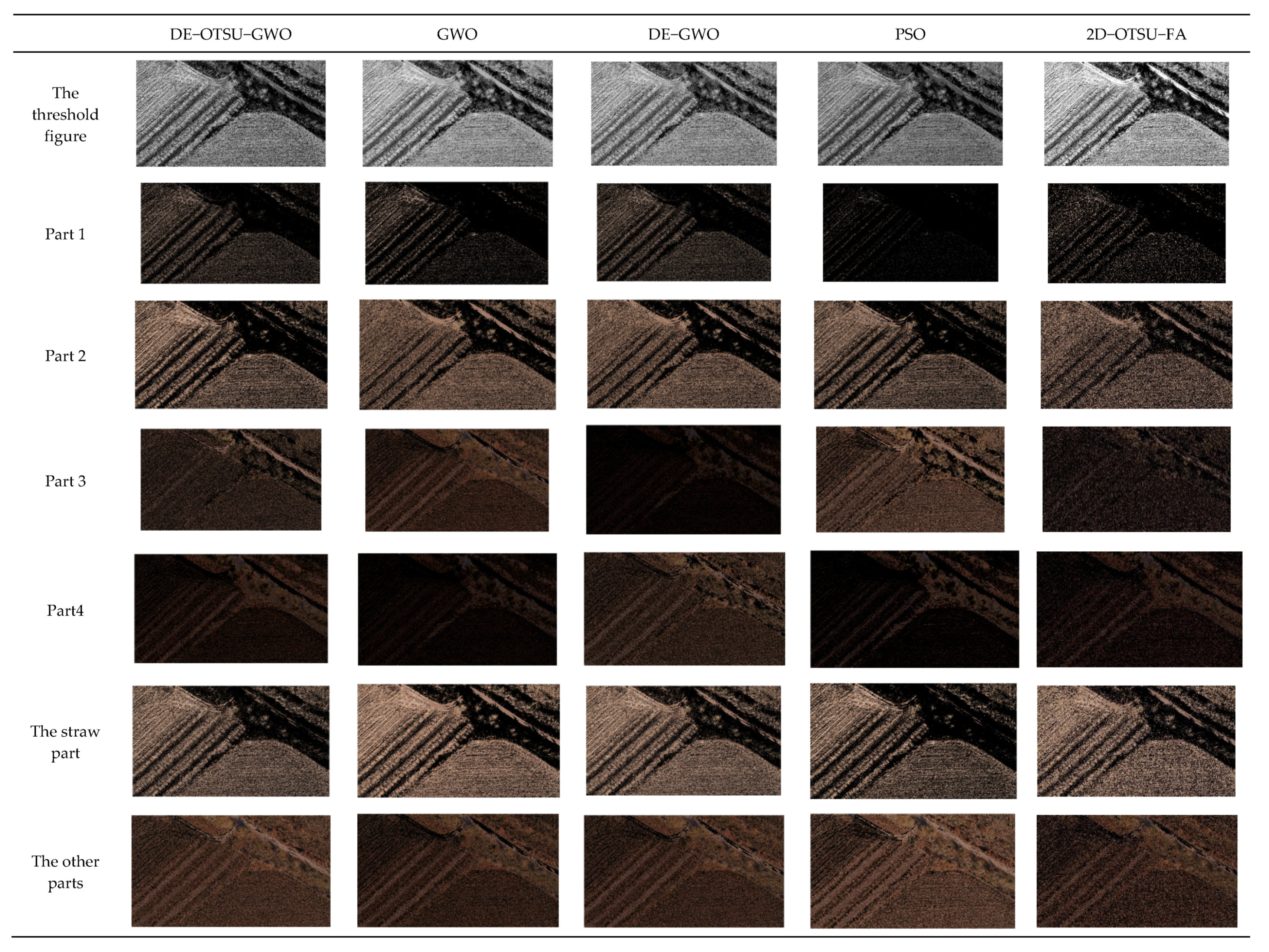
To test the effectiveness of the algorithm, the segmentation effects of PSO, GWO, DE−GWO, DE−OTSU−GWO, and 2D−OTSU−FA were compared. To calculate the straw coverage, it is necessary to divide the straw part and the other parts. The five algorithms are all calculation units of three thresholds. Part 1 and part 2 are the straw part, and part 3 and part 4 are the other parts.

Figure 5 shows the original straw image with a height of 100 m. The overall pixel value is 15,681,600.

The segmentation results of five algorithms are listed in

Table 6. The segmentation results of five algorithms.

Algorithms	The Threshold Value	Pixel Values of Part 1	Pixel Values of Part 2	Pixel Values of Part 3	Pixel Values of Part 4	Straw Pixel Value	Other Pixel Values
DE−OTSU−GWO	86/133/178	2,170,336	3,476,676	4,661,703	5,372,885	5,647,012	10,034,588
GWO	61/115/169	2,760,445	4,767,392	4,938,550	3,215,213	7,527,837	8,153,763
DE−GWO	58/123/176	2,298,200	4,509,371	5,970,221	2,903,808	6,807,571	8,874,029
PSO	74/135/192	269,978	4,596,620	7,654,152	3,160,850	4,866,598	100,815,002
2D−OTSU−FA	84/121/193	1,280,279	5,736,297	3,567,160	5,097,864	7,016,576	86,650,024

.

Figure 6 shows the image segmentation of the five algorithms. It can be seen that GWO, DE−GWO, and 2D−OTSU−FA misjudged the road as straw. Compared with the PSO algorithm, the DE−OTSU−GWO algorithm has a better segmentation effect.

Figure 7 is a small image taken from an image with a height of 30 m. The white box is the location of the detailed diagram in Figure 8. The overall pixel value is 112,810.

The segmentation results of the five algorithms are listed in

Table 7. The segmentation results of five algorithms.

Algorithms	The Threshold Value	Pixel Values of Part 1	Pixel Values of Part 2	Pixel Values of Part 3	Pixel Values of Part 4	Straw Pixel Value	Other Pixel Values
DE−OTSU−GWO	123/161/228	969	8384	20,927	82,530	9353	103,457
GWO	71/140/199	2974	14,653	61,276	33,907	17,627	95,183
DE−GWO	49/145/189	4144	10,983	75,835	21,848	15,127	97,683
PSO	71/148/206	2296	11,483	64,488	34,543	13,779	99,031
2D−OTSU−FA	97/145/192	3886	11,241	43,542	54,141	15,127	97,683

.

Figure 8 shows the image segmentation of the five algorithms. It can be seen that GWO, DE−GWO, PSO, and 2D−OTSU−FA can also divide the straw part, however, the four algorithms misjudge the land as straw. The DE−OTSU−GWO has a better segmentation effect in comparison with the other four algorithms.

The sensitivity generated by the integration of each algorithm can be seen from the influence of the algorithm on the whole. The sensitivity C is as follows:

$$C=\left|\frac{F\left(x+y\right)-F\left(x\right)}{F\left(x+y\right)}\right|$$

(31)

If $C$ is large, then $F\left(x\right)$ is stable. If $C$ is small, then $F\left(x\right)$ is sensitive.

Table 8. Results of DE−OTSU−GWO algorithm analysis.

Algorithms	The Threshold Value	Relative Value	T(n)	Time Consumption
DE−OTSU−GWO	123/161/228	−−	O(18n4+2n3+10n2+6n)	2.743333
GWO	71/140/199	0.422/0.130/0.127	O(4n3)	1.931997
DE−GWO	49/145/189	0.601/0.099/0.171	O(18n4+11n3+2n2)	0.220224
OTSU−GWO	72/142/202	0.414/0.118/0.114	O(4n3+8n2)	3.654632

lists the analysis results for the DE−OTSU−GWO algorithm. For the first and the third thresholds, OTSO−GWO is sensitive compared with GWO and DE−GWO, and the difference is obvious. In the second threshold, DE−GWO is sensitive compared with OTSU−GWO, but the difference is insignificant. T(n) is time complexity. The size of the loop n of the algorithm is different, therefore, T(n) cannot directly represent the time consumption. After adding the DE algorithm, although the time complexity increases by O(18n⁴), it reduces the time to solve the local optimal solution of the GWO algorithm. The OTSU algorithm needs to traverse each grey value and classify it; the overall time is increased. For example, when the DE−OTSU−GWO algorithm processes Figure 7 as configured in Section 3, the processing time is within the acceptable range.

Figure 9 shows the manual segmentation of straw using Adobe Photoshop software.

A number of parameters can be used to assess the segmentation. In this paper, the global consistency error (GCE) [35], random index (RI) [36], and variation of information (VI) [37] are used to compare the segmentation results. If GCE and VI are high, then there is a significant difference in segmentation. If GEC and VI are low, then there is a slight difference. RI means the opposite of GCE and VI [38]. GCE, RI, and VI are shown below. (The use of the formula symbol in this section is shown in

Table 9. The implication of the formula symbol in Section 4.

Symbol	Implication	Symbol	Implication
$F\left(x\right)$	The threshold of algorithm x	$i$	label
n	Scale of problem	${\displaystyle \sum }_i{n}_{ij}$	the number of points with $i$ in the $S$
T(n)	Time frequency	${\displaystyle \sum }_j{n}_{ij}c$	the number of points with $j$ in the $S^{\prime }$
$S_1$ and $S_2$	Segmentation	$N$	the total number of points
$p_q$	pixel	$C$	clustering
$R\left(S,p_q\right)$	a region in segmentation $S$ with $p_q$	$H\left(C\right)$	Entropy of $C$
$n$	the number of pixels	$I\left(C_1,C_2\right)$	the mutual information between $C_1$ and $C_2$

).

$$E\left(S_1,S_2,p_q\right)=\frac{\left|R\left(S_1,p_q\right)\backslash R\left(S_2,p_q\right)\right|}{\left|R\left(S_1,p_q\right)\right|}$$

(32)

$$GCE\left(S_1,S_2\right)=\frac{1}{n}\min \left\{\sum _{i}E\left(S_1,S_2,p_q\right),\sum _{i}E\left(S_2,S_1,p_q\right)\right\}$$

(33)

$$RI\left(S,S^{\prime }\right)=1-\frac{\left[\frac{1}{2}\left\{{\sum }_i{\left({\sum }_j{n}_{ij}\right)}^2+{\sum }_j{\left({\sum }_i{n}_{ij}\right)}^2\right\}-{\sum }^{ }{\sum }^{ }{n}_{ij}\right]}{\left(\begin{array}{c}N\\ 2\end{array}\right)}$$

(34)

$$VI\left(C_1,C_2\right)=\left[H\left(C_1\right)-I\left(C_1,C_2\right)\right]+\left[H\left(C_2\right)-I\left(C_1,C_2\right)\right]$$

(35)

Table 10. The assessment results of segmentation.

Algorithms	The Threshold Value	RI	GCE	VI
DE−OTSU−GWO	123/161/228	0.9493	0.0518	0.3095
GWO	71/140/199	0.8930	0.0633	0.3950
DE−GWO	49/145/189	0.9196	0.0609	0.3627
PSO	71/148/206	0.9328	0.0596	0.3448
2D−OTSU−FA	97/145/192	0.8885	0.0680	0.4043

lists the assessment results of segmentation. The manual segmentation image is regarded as the gold standard image. Compared with GWO, DE−GWO, PSO, and 2D−OTSU−FA, the DE−OTSU−GWO algorithm has better results in the detection of RI, GCE, and VI. This indicates that the segmentation results of the DE−OTSU−GWO algorithm are close to the results of manual detection. According to the data in Table 8 and Table 10, it can be seen that the OTSU algorithm is improved compared with the other four algorithms in terms of accuracy, although it increases in time. The combination of DE and GWO can solve the local optimal solution problem and reduce time consumption.

5. Conclusions

There have been a number of improved grey wolf optimizer (GWO) algorithms in recent years, including an improved GWO algorithm for initial population selection and threshold selection. This paper proposed an improved GWO algorithm based on the differential evolution (DE) algorithm and the OTSU algorithm. The GWO algorithm combines multithreshold OTSU, Tsallis entropy, and DE algorithms. Multithreshold OTSU calculates the fitness in the initial population and makes the initial stage basically stable, and not affected by image brightness and contrast. Tsallis entropy quickly calculates the fitness. The DE algorithm can solve the local optimal solution of the GWO algorithm.

The performance of the DE−OTSU−GWO algorithm was tested using a CEC2005 benchmark function (23 test functions). Compared with existing PSO and GWO algorithms, the experimental results showed that the DE−OTSU−GWO algorithm is more stable and accurate in solving benchmark functions. In addition, compared with other algorithms, a convergence behavior analysis proved the high quality of the DE−OTSU−GWO algorithm.

In the results of classical agricultural image recognition problems, compared with GWO, PSO, DE−GWO, and 2D−OTSU−FA, the DE−OTSU−GWO algorithm had accuracy in straw image recognition and is applicable to practical problems. In the sensitivity detection of each algorithm, for the first and the third thresholds, the OTSO−GWO is sensitive compared with GWO and DE−GWO, and the difference is obvious. In the second threshold, the DE−GWO is sensitive compared with OTSU−GWO, but the difference is insignificant. In terms of time complexity, after adding the DE algorithm, the time complexity increases by O(18n⁴). However, the OTSU algorithm needs to traverse each grey value and classify it, so the overall time is increased. Adding the DE algorithm can solve the local optimal solution of GWO and the time will be reduced. Compared with GWO, DE−GWO, PSO, and 2D−OTSU−FA, the DE−OTSU−GWO algorithm has better results in the detection of RI, GCE, and VI. The segmentation results of the DE−OTSU−GWO algorithm are close to the results of manual detection.

References

1. Roberts, M.; Chen, K.; Irion, K.L. A convex geodesic selective model for image segmentation. J. Math. Imaging Vis. 2019, 61, 482–503. [Google Scholar] [CrossRef] [Green Version]
2. Guo, F.F.; Wang, X.X.; Shen, J. Adaptive fuzzy c-means algorithm based on local noise detecting for image segmentation. IET Image Process. 2016, 10, 272–279. [Google Scholar] [CrossRef]
3. Benninghoff, H.; Garcke, H. Image segmentation and restoration using parametric contours with free endpoints. IEEE Trans. Image Process. 2016, 25, 1639–1648. [Google Scholar] [CrossRef] [PubMed] [Green Version]
4. Banerjee, A.; Maji, P. Rough sets and stomped normal distribution for simultaneous segmentation and bias field correction in brain MR Images. IEEE Trans. Image Process. 2015, 24, 5764–5776. [Google Scholar] [CrossRef]
5. Kurmi, Y.; Chaurasia, V. Multifeature-based medical image segmentation. IET Image Process. 2018, 12, 1491–1498. [Google Scholar] [CrossRef]
6. Konstantopoulos, C.; Mamalis, B.; Pantziou, G.; Thanasias, V. An image processing inspired mobile sink solution for energy efficient data gathering in wireless sensor networks. Wirel. Netw. 2015, 21, 227–249. [Google Scholar] [CrossRef]
7. Liu, C.; Zhou, A.; Zhang, Q.; Zhang, G. Adaptive image segmentation by using mean-shift and evolutionary optimisation. IET Image Process. 2014, 8, 327–333. [Google Scholar] [CrossRef]
8. Dhara, A.K.; Mukhopadhyay, S.; Chakrabarty, S.; Garg, M.; Khandelwal, N. Quantitative evaluation of margin sharpness of pulmonary nodules in lung CT images. IET Image Process. 2016, 10, 631–637. [Google Scholar] [CrossRef]
9. Chen, L.C.; Papandreou, G.; Kokkinos, I.; Murphy, K.; Yuille, A.L. Deeplab: Semantic image segmentation with deep convolutional nets, atrous convolution, and fully connected crfs. IEEE Trans. Pattern Anal. Mach. Intell. 2018, 40, 834–848. [Google Scholar] [CrossRef]
10. Panagiotakis, C.; Argyros, A. Region-based fitting of overlapping ellipses and its application to cells segmentation. Image Vis. Comput. 2020, 93, 1–30. [Google Scholar] [CrossRef]
11. Grigoryan, A.M.; Agaian, S.S. Monotonic sequences for image enhancement and segmentation. Digit. Signal Process. 2015, 41, 70–89. [Google Scholar] [CrossRef]
12. Lu, Y.; Lu, R. Histogram-based automatic thresholding for bruise detection of apples by structured-illumination reflectance imaging. Biosyst. Eng. 2017, 160, 30–41. [Google Scholar] [CrossRef]
13. Zhang, P.; Lu, S.; Li, J.; Zhang, P.; Xie, L.; Xue, H.; Zhang, J. Multi-component segmentation of X-ray computed tomography (CT) image using multi-Otsu thresholding algorithm and scanning electron microscopy. Energy Explor. Exploit. 2017, 35, 281–294. [Google Scholar] [CrossRef] [Green Version]
14. Shannon, C.E. A Mathematical Theory of Communication. Bell Syst. Tech. J. 1948, 27, 379–423. [Google Scholar] [CrossRef] [Green Version]
15. Otsu, N. A threshold selection method from gray-level histograms. IEEE Trans. Syst. Man Cybern. 1979, 9, 62–66. [Google Scholar] [CrossRef] [Green Version]
16. Kapur, J.N.; Sahoo, P.K.; Wong, A.K.C. A new method for gray-level picture thresholding using the entropy of the histogram. Comput. Vis. Graph. Image Process. 1985, 29, 273–285. [Google Scholar] [CrossRef]
17. Liu, J.Z.; Li, W.Q. Two-dimensional Otsu automatic threshold segmentation of grayscale image. Acta Autom. 1993, 19, 101–105. [Google Scholar]
18. Holland, J.H. Genetic algorithms. Sci. Am. 1992, 267, 66–72. [Google Scholar] [CrossRef]
19. Eberhart, R.C.; Kennedy, J. A new optimizer using particle swarm theory. In Proceedings of the Sixth International Symposium, Micro Machine and Human Science (MHS’95), Nagoya, Japan, 4–6 October 1995; IEEE: Piscataway, NJ, USA, 1995. [Google Scholar]
20. Mirjalili, S.; Mirjalili, S.M.; Lewis, A. Grey Wolf Optimizer. Adv. Eng. Softw. 2014, 69, 46–61. [Google Scholar] [CrossRef] [Green Version]
21. Zahara, E.; Fan, S.K.S.; Tsai, D.M. Optimal multi-thresholding using a hybrid optimization approach. Pattern Recognit. Lett. 2005, 26, 1082–1095. [Google Scholar] [CrossRef]
22. Cui, B.X.; Wang, H.; Duan, Y. Fire image segmentation based on improved two-dimensional Otsu thresholding method and PSO. Shenyang Gongye Daxue Xuebao/J. Shenyang Univ. Technol. 2010, 32, 75–78+89. [Google Scholar]
23. Helen, R.; Kamaraj, N.; Selvi, K.; Raman, V.R. Segmentation of pulmonary parenchyma in CT lung images based on 2D Otsu optimized by PSO. In Proceedings of the 2011 International Conference on Emerging Trends in Electrical and Computer Technology, Nagercoil, India, 23–24 March 2011. [Google Scholar]
24. Hamdaoui, F.; Sakly, A.; Abdellatif, M. An efficient multi level thresholding method for image segmentation based on the hybridization of modified PSO and Otsu’s method. Comput. Inf. Sci. 2015, 575, 343–367. [Google Scholar]
25. Khairuzzaman, A.K.M.; Chaudhury, S. Multilevel thresholding using grey wolf optimizer for image segmentation. Expert Syst. Appl. 2017, 86, 64–76. [Google Scholar] [CrossRef]
26. Ibrahim, R.A.; Elaziz, M.A.; Lu, S. Chaotic opposition-based grey-wolf optimization algorithm based on differential evolution and disruption operator for global optimization. Expert Syst. Appl. 2018, 108, 1–27. [Google Scholar] [CrossRef]
27. Bohat, V.K.; Arya, K.V. A new heuristic for multilevel thresholding of images. Expert Syst. Appl. 2019, 117, 176–203. [Google Scholar] [CrossRef]
28. Zhou, C.; Tian, L.; Zhao, H.; Zhao, K. A method of two-dimensional Otsu image threshold segmentation based on improved firefly algorithm. In Proceedings of the 2015 IEEE International Conference on Cyber Technology in Automation, Control, and Intelligent Systems (CYBER), Shenyang, China, 8–12 June 2015; pp. 1420–1424. [Google Scholar]
29. Kao, Y.H.; Teng, M.M.; Zheng, W.Y.; Chang, F.C.; Chen, Y.F. Removal of csf pixels on brain mr perfusion images using first several images and otsu’s thresholding technique. Magn. Reson. Med. 2010, 64, 743–748. [Google Scholar] [CrossRef]
30. Tan, Z.G.; Ou, J.P.; Zhang, J.; Shen, X.G. Depth image segmentation algorithm based on multi-feature combination. Comput. Eng. Sci. 2018, 40, 97–102. [Google Scholar]
31. Zhang, X.M.; Zhang, B.; Tu, Q. Fast multi-threshold image segmentation based on generalized probability Tsallis entropy. Data Acquis. Process. 2016, 31, 502–511. [Google Scholar]
32. Storn, R.; Price, K. Differential evolution—A simple and efficient heuristic for global optimization over continuous spaces. J. Glob. Optim. 1997, 11, 341–359. [Google Scholar] [CrossRef]
33. Suganthan, P.N.; Hansen, N.; Liang, J.; Deb, K.; Chen, Y.P.; Auger, A.; Tiwari, S. Problem Definitions and Evaluation Criteria for the CEC 2005 Special Session on Real-Parameter Optimization; Technical Report; Natural Computing; Nanyang Technological University: Singapore, 2005; pp. 341–357. [Google Scholar]
34. Tawhid, M.A.; Ibrahim, A.M. A hybridization of grey wolf optimizer and differential evolution for solving nonlinear systems. Evol. Syst. 2020, 11, 65–87. [Google Scholar] [CrossRef]
35. Martin, D.; Fowlkes, C.; Tal, D.; Malik, J. A database of human segmented natural images and its application to evaluating segmentation algorithms and measuring ecological statistics. In Proceedings of the IEEE International Conference on Computer Vision, Vancouver, BC, Canada, 7–14 July 2001. [Google Scholar]
36. Rand, W.M. Objective Criteria for the Evaluation of Clustering Methods. J. Am. Stat. Assoc. 1971, 336, 846–850. [Google Scholar] [CrossRef]
37. Meila, M. Comparing clusterings by the variation of information. In Learning Theory and Kernel Machines; Lecture Notes in Computer Science; Springer: Berlin/Heidelberg, Germany, 2003; Volume 2777, pp. 173–187. [Google Scholar]
38. Khan, M.B.; Nisar, H.; Ng, C.A.; Ali, Y.; Malik, A. Segmentation assessment of activated sludge flocs at different magnifications for wastewater treatment. In Proceedings of the IEEE International Conference on Control System 2014, Batu Ferringhi, Malaysia, 28–30 November 2014. [Google Scholar]
Figure 1. The flowchart of DE-OTSU-GWO algorithm.
Applsci 10 06343 g001
Figure 2. The pseudo-code of DE-OTSU-GWO algorithm.
Applsci 10 06343 g002
Figure 3. The 2D version of the benchmark functions.
Applsci 10 06343 g003aApplsci 10 06343 g003b
Figure 4. The changes in the iterative process of the three algorithms.
Applsci 10 06343 g004
Figure 5. Original straw image with the height of 100 m.
Applsci 10 06343 g005
Figure 6. Image segmentation of five algorithms with the height of 100 m.
Applsci 10 06343 g006
Figure 7. Original straw image with the height of 30 m.
Applsci 10 06343 g007
Figure 8. Image segmentation of five algorithms with the height of 30 m.
Applsci 10 06343 g008
Figure 9. Manual segmentation of straw.
Applsci 10 06343 g009