Autonomous Vehicles: Vehicle Parameter Estimation Using Variational Bayes and Kinematics

Abstract

On-board sensory systems in autonomous vehicles make it possible to acquire information about the vehicle itself and about its relevant surroundings. With this information the vehicle actuators are able to follow the corresponding control commands and behave accordingly. Localization is thus a critical feature in autonomous driving to define trajectories to follow and enable maneuvers. Localization approaches using sensor data are mainly based on Bayes filters. Whitebox models that are used to this end use kinematics and vehicle parameters, such as wheel radii, to interfere the vehicle’s movement. As a consequence, faulty vehicle parameters lead to poor localization results. On the other hand, blackbox models use motion data to model vehicle behavior without relying on vehicle parameters. Due to their high non-linearity, blackbox approaches outperform whitebox models but faulty behaviour such as overfitting is hardly identifiable without intensive experiments. In this paper, we extend blackbox models using kinematics, by inferring vehicle parameters and then transforming blackbox models into whitebox models. The probabilistic perspective of vehicle movement is extended using random variables representing vehicle parameters. We validated our approach, acquiring and analyzing simulated noisy movement data from mobile robots and vehicles. Results show that it is possible to estimate vehicle parameters with few kinematic assumptions.

1. Introduction

The behavior of autonomous vehicles is strongly reliant on their sensors’ data and the interpretation of the environment [1]. Internal sensors can be used to estimate the vehicle’s own movement and assist in their control. However, due to sensor noise, external information needs to be used from perception approaches. These data enable the correction of assumptions based solely on internal sensors, increasing the accuracy and reliability of the active safety systems through knowledge of the vehicle’s surroundings (e.g., through object recognition and tracking).

One of the main characteristics of an autonomous vehicle is the ability to localize itself. To make localization possible a function $f:\Delta \Phi \mapsto \mathcal{X}$ is needed (see Equation (1)) which maps for m wheels the angular rotation $\Delta \Phi =\left\{\begin{array}{c}\Delta {\varphi }_0,\Delta {\varphi }_1,\cdots ,\Delta {\varphi }_m\end{array}\right\}$ and vehicle parameters $\Theta$ to a new vehicle pose. In this study, we summarize wheel radii, and distances between wheels used for kinematic models as “vehicle parameters”.

To estimate movement for a two-wheeled vehicle on a two dimensional surface at time t, following general notation can be used:

$${\left(\begin{array}{c}\Delta x\\ \Delta y\\ \Delta \theta \end{array}\right)}_t=f(\Delta {\varphi }_l,\Delta {\varphi }_r,\Theta )$$

(1)

Equation (1) calculates pose changes based on the left wheel motion $\Delta {\varphi }_l$, the right wheel motion $\Delta {\varphi }_r$ and vehicle parameter $\Theta$. Since a vehicle is a machine that transports people or goods from one place to another [2] and a robot is a machine capable of carrying out a complex series of actions automatically [3], we can define autonomous vehicles as vehicular robots. From a mathematical perspective, both terminologies are equivalently described using f, since both models are fully described by analyzing the wheel motion. The function f is also known as motion model. Motion models are crucial for autonomous vehicles since they are utilized in control, perception and planning [4]. The most commonly used motion models are based on either constant turn rate, constant acceleration, constant velocity or on a combination of these [5].

The angular movement of the wheels and the vehicle parameters $\Theta$ (wheel radii and distance between wheels) are used to calculate the pose of the vehicle. This use of data from the movement of actuators to estimate changes in position over time is defined as odometry. A well documented issue with odometry is imprecision/inaccuracy, since wheels tend to slip on the road’s surface [6]. Therefore the previously defined f function is not adequate to estimate these changes.

To alleviate uncertainty (noise) and unknown effects that disturb rather theoretical kinematic models and produce errors [7], probabilistic approaches have been developed to enable localization under uncertainty in real environments. Some of them are summarized in [1].

Applying a probabilistic approach, the function in Equation (1) is able to map the wheel rotation to the pose changes and to merge vehicle parameters, such as wheel radii, as unknown parameters using black box approaches [8,9].

Probabilistic models are used to determine coherences and marginal distributions [10] and can be described using graphical representations [11]. As a special instantiation, hidden Markov models [12] are the base for Bayes filters [1], which are the main models used for vehicle localization. The goal of a Bayes filter is to fuse information, where a movement model $p\left({\overrightarrow{x}}_t\right|{\overrightarrow{x}}_{t-1},{\overrightarrow{u}}_t)$, a measurement model $p\left({\overrightarrow{z}}_t\right|{\overrightarrow{x}}_t)$, the vehicle’s last state ${\overrightarrow{x}}_{t-1}$ at the time slot $t-1$, as well as the so-called command value ${\overrightarrow{u}}_t$ and measurements ${\overrightarrow{z}}_t$ to the latest vehicle pose ${\overrightarrow{x}}_t$ at the time step t.

Compared to simple odometry, Bayes filters have the advantage of being able to represent the uncertainty along a predicted trajectory. To better understand the complexity of Bayes filters, probabilistic graphical models can describe the localization approach [11,13] as shown for example in Figure 1, in which the arrows represent the conditional (in)dependency and conditional probabilities. Note that the Bayes filter does not define the vehicle parameters, sensor technology or control input.

The most common choice of Bayes filter implementation is the Kalman filter (KF) [14,15]. The KF is based on linear movement and measurement models. Since this is a strong restriction for real applications, several extensions exists. Generic algorithms and non-linear KF [16,17] were previously implemented to overcome this restriction. A methodology for federated KF in order to implement a self-adaptive navigation system was implemented in [18]. The unscented transformation was proposed in [19] for non-linear function approximation.

However, in order to learn non-linear and non-parametric movement models from real data, Bayes filters based on advanced statistical models rather than linear movement models which are used in Kalman filters were implemented [8,9].

Unfortunately, due to their high non-linearity, those models tend to become blackbox models that deliver the expected outputs without having any in-depth knowledge of the internal processes structure. Intensive experiments are needed to analyze the system behavior, which is not a trivial task [10,20].

This work is motivated by the need for explainable machine learning solutions for safety critical systems. The importance of a fundamental understanding of any artificial intelligence based system has been highlighted in [21]. The authors argued that this can only be achieved by the identification of underlying explanatory factors. Several machine learning models such as artificial neuronal networks cannot identify causal relations in data and thus cannot fully understand the environment [20]. To identify causality more appropriate approaches exist that rely on Bayesian methodologies, as described in [10]. Approaches that are based on Bayesian methods have some similarities with Gaussian processes (GP). For example, specific families of Bayesian artificial neuronal networks with an infinite number of neurons converge to Gaussian processes [22].

Relying on this information, the study presented in this work is based on GPs due to the non-parametric nature of the model. This means that GP models are able to perform predictions without requiring user-based definitions, contrary for example to other machine learning models that base on neuronal network architectures and affect the model performance significantly.

Therefore, since user-based definitions would critically limit the explanatory power of the presented methodology, parametric models such as artificial neuronal networks will not be the focus of this work.

$p\left({\overrightarrow{x}}_t\right|{\overrightarrow{x}}_{t-1},{\overrightarrow{u}}_t)$ and $p\left({\overrightarrow{z}}_t\right|{\overrightarrow{x}}_t)$ were previously implemented in [8,23,24] using Gaussian processes [25]. Those GP-based localization approaches [8,23,24] tackle the problem of modelling movement and measurement models based on data and machine learning. The resulting models are called blackbox models, since they deliver the outputs without having any in-depth knowledge of the internal processes structure. In general, these GPs are based on a dataset of n examples described by $\mathcal{D}=\{(y_0,{\overrightarrow{x}}_0),\cdots ,(y_n,{\overrightarrow{x}}_n)\}$. Prediction and subsequent integration in localization applications is achieved using data similarity, which is implemented using kernels [26]. The prediction of the vehicle movement $y^{*}$ can be calculated using wheel movement ${\overrightarrow{x}}^{*}$. The noise-free prediction of $y^{*}$ is depicted by $f^{*}$ and is estimated using the following Equation (2), which has been previously discussed in [25].

$$\left(\begin{array}{c}\overrightarrow{y}\\ f^{*}\end{array}\right)\sim \mathcal{N}\left(\begin{array}{c}\overrightarrow{0},\left[\begin{array}{cc}\mathbf{K}+{\sigma }_n^2\mathbf{I}& {\overrightarrow{k}}_{*}^T\\ {\overrightarrow{k}}_{*}& k_{**}\end{array}\right]\end{array}\right).$$

(2)

In the equation $\mathbf{K}$ is an elementwise similarity measurement, ${\overrightarrow{k}}_{*}$ describes the similarity of a new input (e.g., wheel movement) to the stored values and $k_{**}$ describes the similarity of the new input to itself. ${\sigma }_n$ is the variance of noise and $\mathbf{I}$ is the identity matrix. Thus a prediction is based on the estimation of $p(f_{*}|\overrightarrow{f},\mathbf{X},{\overrightarrow{x}}_{*})$ and is done rearranging Equation (2). For GP-based localization, two GP are used to model $p\left({\overrightarrow{x}}_t\right|{\overrightarrow{x}}_{t-1},{\overrightarrow{u}}_t)$ and $p\left({\overrightarrow{z}}_t\right|{\overrightarrow{x}}_t)$. To describe those models a compact notation of Equation (2) is used:

$$\begin{array}{cc}\hfill p\left({\overrightarrow{x}}_t\right|{\overrightarrow{x}}_{t-1},{\overrightarrow{u}}_t)& =\mathcal{N}\left(\begin{array}{c}G{P}_{\mu }({\overrightarrow{x}}_{t-1},{\overrightarrow{u}}_t,{\mathcal{D}}_p),G{P}_{\Sigma }({\overrightarrow{x}}_{t-1},{\overrightarrow{u}}_t,{\mathcal{D}}_p)\end{array}\right)\hfill \end{array}$$

(3)

$$\begin{array}{cc}\hfill p\left({\overrightarrow{z}}_t\right|{\overrightarrow{x}}_t)& =\mathcal{N}\left(\begin{array}{c}G{P}_{\mu }({\overrightarrow{x}}_t,{\mathcal{D}}_o),G{P}_{\Sigma }({\overrightarrow{x}}_t,{\mathcal{D}}_o)\end{array}\right)\hfill \end{array}$$

(4)

where the functions $G{P}_{\mu }(.)={\overrightarrow{k}}_{*}{(\mathbf{K}+{\sigma }_n^2\mathbf{I})}^{-1}\overrightarrow{y}$ and $G{P}_{\Sigma }(.)=\mathbf{K}-{\overrightarrow{k}}_{*}{(\mathbf{K}+{\sigma }_n^2\mathbf{I})}^{-1}{\overrightarrow{k}}_{*}$ are the GP prediction functions [26].

However, even if GP-based localization can outperform classic approaches, physics-based motion models (e.g., whitebox models) remain the most reliable movement models for trajectory prediction and collision risk estimation for road safety. Their reliability as well as the fact that they rely solely on movement properties and do not include any inertial properties has led to their widespread use [27]. Physics-based trajectory prediction algorithms can only be used in low speed situations and are limited to short-term forecasting [27,28]. Therefore, one of the big challenges of these algorithms is to identify and quantify the potential and limitations of their agents in order to integrate this knowledge into their maneuvers and trajectories [29] for the sake of road safety.

To contribute to the field of research, we define the following null hypothesis:

H0: 

sGP-based motion models are not able to learn movement based on wheel motion.

That we will test by converting blackbox models (e.g., GP motion models) to whitebox models, in which the internal processes can be viewed by using simple kinematic models.

We estimate the kinematic parameters wheel baseline B, radii r and distance between rear and front wheels T which need to be derived from the GP models. The model performance in terms of motion accuracy (X, Y and $\theta$) is not focus of this study.

We contribute to the state of the art through the extension of a Gaussian process-based [25] localization approach [8] that estimates movement models without vehicle parameters. Based on the movement model, we derive wheel radii and distances and are thereby able to analyze the model behavior using physical plausibility. Thus, we evaluate our approach by comparing the derived vehicle parameters to simulated ground truth data vehicle parameter. To this end, we (i) introduce a Bayesian perspective of a motion model using approximate GP inference and (ii) then deduct the correspondent vehicle parameters as random variables.

The non-parametric GP model learns movement models based on data. Explanatory factors such as wheel radii are learned implicitly. Thus, the explanatory factors must be derived from GP models afterwards. To implement this derivation, we extend existing approaches such as [30] by introducing a kinematic model to our derivation. Additionally, as an alternative to approaches based on classic control-theory such as [31], we use recent non-linear methodologies as motion models.

Our approach is summarized in Figure 2 for a mobile robot. We use on-board sensor data (green variables) and global movement data to estimate a GP based movement model. For this study, wheel encoder and global vehicle pose were used. Based on the GP models, we derive kinematic vehicle parameters (red variables) such as wheel radii and distances. The method proposed in this work intends to estimate the pertinent vehicle parameters resulting from machine learning algorithms and validate them using simulated ground truth data. For the purpose of this study, we chose two different kinematic models, namely the Ackermann steering and the differential-driven vehicle to prove our approach. We chose those kinematic models due to existing autonomous cars (e.g., Waymo https://waymo.com/), AGV (e.g., Mir (see https://www.mobile-industrial-robots.com/de/solutions/robots/mir100/) or SALLY (see https://www.ds-automotion.com/en/solutions/ats-agv/sally-courier/?L%5B0%5D=title%3DOffre)) or scientific/educational plattforms (e.g., Turtlebot (see https://www.turtlebot.com/)). The implemented methodology in the presented work contributes to the state of the art by adding new insights to motion models based on sGP. The presented approach for explanatory factor extraction of blackbox motion models has not been implemented until the present day.

This work is structured as follows: The next chapter discusses several Bayes filter implementations and novel approaches in the context of autonomous driving. The methodological approach through the introduction of additional vehicle parameters for a fully Bayesian perspective, the validation approach and the comparison of blackbox and whitebox models are presented in Section 3. Section 4 presents the results from the applied methodology. Finally, in Section 5 we conclude the paper and indicate future research.

2. State of the Art

One of the main challenges in complex system modelling is the explainability of the methods and processes that are internally executed and determining which elements serve as the basis for a later analyzis of the model behavior. Several works have been dedicated to solving the problem of retracing the algorithmic behaviour. For example, the authors in [32] proposed methods for visualizing the behavior of deep neural nets. Additionally, the work in [33,34] used statistical optimization criteria for variational Bayes [35] based approaches. In the same line of research, in [10,11] the authors introduced approaches for causal inference in Bayes networks. Despite these efforts, the physical interpretation is still difficult and typically not performed in the related literature. Therefore, we contribute to the state of the art by introducing a novel kinematic-based approach that makes it possible to relate the learning data to the behavior of machine learning-based motion models. The approach presented in this work relies on classic approaches for localization, novel machine learning algorithms and non-parametric statistics. Therefore, we initially discuss classic localization approaches and focus then on progress in Gaussian process modeling.

2.1. Bayesian State Estimation Approaches

To define the likelihood function required for Bayes filters, several implementations have been proposed in the literature. For example, the authors in [36] developed a Kalman filter framework that provided accurate estimates of vehicle position, velocity and altitude (5–10 centimeter root mean square (RMS)). The approach was evaluated using a dataset containing over 60 km of highway and dynamic urban scenes in which the global navigation satellite system (GNSS) reception ranged from good to weak/none. The developed multi-sensor fusion algorithm adaptively utilized diverse localization approaches based on inertial measurement unit (IMU), real time kinematic (RTK) and light detection and ranging (LIDAR) sensors.

An Extended Kalman Filter Dead Reckoning (EKFDR) approach to tackle the ego-localization problem in areas of weak GPS reception was presented in [37]. The developed EKFDR corrects both deterministic (e.g., production-related) and stochastic (e.g., slip due to wet road) errors based on a novel Map Matching (MM) algorithm that reduces both the cross- and along track errors. This new MM approach is used in the correction step of the EKFDR to update the state propagation. Doing so they achieved a maximum error of 15.4 m and an average error of 5.2 m during a 43 km long test drive, thus outperforming low-cost GPS systems. EKF can also be used to localize multiple robots at the same time.

A recursive Interim Master Decentralized Cooperative Localization (D-CL) localization approach for a swarm or robots was presented in [38]. Here the state prediction is completely decoupled, thus no communication between the robots is needed during this step. Intra-network communication is only needed in the update step of the EKF if a relative measurement between two robots is made. The robot that produced the relative measurement is declared as the interim master and utilizes the data provided by the landmark robot to calculate the update variables for the other robots.

Another novel approach for the bayesian state estimator Particle Filter (PF) was introduced in [39]. The authors of this work proposed a map-relative PF based localization for autonomous unmanned air vehicles (UAV) with a downward facing camera. Similarity calculation using the Pearson Correlation Coefficient, between map and aerial images that were converted to probability distributions using image similarity to likelihood conversion function, were used as input for the PF. Evaluation on a simulated dataset showed that the proposed method outperformed state of the art ORB-SLAM2 with an 2.6 times higher average precision.

A further work [40] introduced a novel approach for PF based localization by combining road intensity (e.g., road markings) and vertical (e.g., trees, street poles or houses) information. The authors assumed that each feature in a previously built map might partially change. Accordingly, they used different measurement models by estimating weights for each particle using an entropy-based cost function. By doing so they adaptively changed the contribution of the intensity and vertical features thus creating a robust localization PF for environments that exhibited changes in its structure. The approach was validated by utilizing a 6 months old high definition map, of a 19 km long urban area, and a survey vehicle and it was compared against several reference localization algorithms and ground truth data. The results showed that the proposed algorithm could outperform other localization algorithms.

A comparison of EKF and PF for simulated GPS and inertial navigation system data can be found in [41].

As the Bayes filter does not define model capabilities, limitations are encoded in the likelihood functions. Since classic approaches such as Kalman Filters use strong assumptions such as Gaussian noise or linear movement models, the work [8] introduces a Gaussian-process (GP) [26] extended Kalman filter and a particle filter for highly nonlinear and accurate Bayes filters using machine learning. Our approach is based on this implementation. Since both the movement and measurement models are used in each timestep in the Bayes filter, the matrix multiplication with $\mathbf{K}\in {\mathbb{R}}^{n\times n}$ must be performed. Since each GP prediction is based on the whole dataset, GPs are typically not useful for real-time applications. Thus, the GP models are “sparsed” or approximated for real time applications.

2.2. Advances in Gaussian-Process Models

Sparsed GP (sGP) approaches tackle the approximation of the full GP using auxiliary variables instead of the similarity measurement $\mathbf{K}$. This can be done using a subset of the training data [42] or pseudo inputs [43,44]. Both approaches aim to identify m variables which can be used instead of n original data points. In the research work in [43] the authors use variational Bayes (VB) [35] as the current state-of-the-art approach for statistical models such as deep GPs [33] or GP latent variable models [34].

This VB-based approximation converts the mean GP prediction procedure to $G{P}_{\mu }(.)={\overrightarrow{k}}_{xm}{\mathbf{K}}_{mm}^{-1}\overrightarrow{\mu }$, where $\overrightarrow{\mu }$ is the result of the approximation procedure and ${\mathbf{K}}_{mm}$ is a similarity matrix of the auxiliary variables. Similar to ${\overrightarrow{k}}_{*}$, ${\overrightarrow{k}}_{xm}\in {\mathbb{R}}^{1xm}$ links the input to the kernel matrix. The number of auxiliary variables needed for the application can be estimated based on the evaluation of the lower bound [35]. Due to the reduction of the training set, where $m\ll n$, the prediction is accelerated.

For autonomous vehicles, sGP can easily be implemented in Bayes filters [8] for movement and measurement models. As we previously mentioned, this results in a black box approach. To overcome this problem, we contribute to the field of research and present in this work a method that combines sGP-based Bayes filters and kinematics to derive vehicle parameters, thereby providing insights on the functionality of sGP in autonomous driving. Our method makes it possible to follow and reproduce the internal processes so that the model behavior can be analyzed later.

3. SGP Motion Model Implementation

To develop the proposed approach of fitting a kinematic model to the sGP motion model, we need to consider the following cases.

• If the derived kinematic model is in accordance with real measurements, the machine learning model will be able to represent the corresponding physical behavior.
• However, if the kinematic model does not rely on data acquired from real-life measurements, the machine learning model might identify incoherences on the sample data that would prevent it from making the appropriate decisions.

Taking this into account, we relied on the work presented in [8] and derived an sGP-based movement model from a data sample. To this end, we used wheel joint movement and simulated ground truth data (X, Y and $\theta$ values). To fit the movement models we used sGP regression to estimate a probabilistic function $f:\Delta {\Phi }_t\mapsto \Delta {\overrightarrow{x}}_{t+1}$ where $\Delta {\Phi }_j={\left(\begin{array}{ccc}\Delta {\varphi }_{l,1}& \cdots & \Delta {\varphi }_{r,n}\end{array}\right)}^T$ includes the wheel joint movements from the time slot $j-1$ to j, describing $\Delta {\overrightarrow{x}}_j$ as the state change from $j-1$ to j.

In addition, the vehicle states are described using ${\overrightarrow{x}}_j={\left(\begin{array}{ccc}x& y& \theta \end{array}\right)}_j^T$. x and y describe the position in a 2D map and $\theta$ denotes the orientation of the vehicle at time j.

Considering that in this work we focus on estimating vehicle parameters instead of improving localization, we decided to use a simplified model as opposed to the one defined above. With the simplified model each movement prediction is based on independent sGP (see Equation (5))

$$\begin{array}{c}\hfill {\left(\begin{array}{c}\mathcal{N}({\mu }_x,{\sigma }_x^2)\\ \mathcal{N}({\mu }_y,{\sigma }_y^2)\\ \mathcal{N}({\mu }_{\theta },{\sigma }_{\theta }^2)\end{array}\right)}_t={\left(\begin{array}{c}sG{P}_x\\ sG{P}_y\\ sG{P}_{\theta }\end{array}\right)}_t\end{array}$$

(5)

where each $sG{P}_j$ is a sparsed Gaussian process, mapping wheel movement and current pose to the new vehicle pose. Note that the vehicle parameters are latent variables in the sGP models and affect each state prediction. To explicitly model the parameters, an additional node can be added to the graphical model (see $\Theta$ in Figure 3).

To perform the analysis, we need to measure the effect of the vehicle parameters rather than the drift. Thus, we perform a virtual vehicle movement using the sGP models, starting from the known vehicle pose ${\overrightarrow{x}}_0={\left(\begin{array}{ccc}0& 0& 0\end{array}\right)}^T$. Since ${\overrightarrow{x}}_0$ is no more a random variable, we can be sure that we measure $\Theta$ rather than the drift or noise. In this procedure (known as clamping), ${\overrightarrow{x}}_t$ becomes independent from the vehicle parameters (Figure 3b).

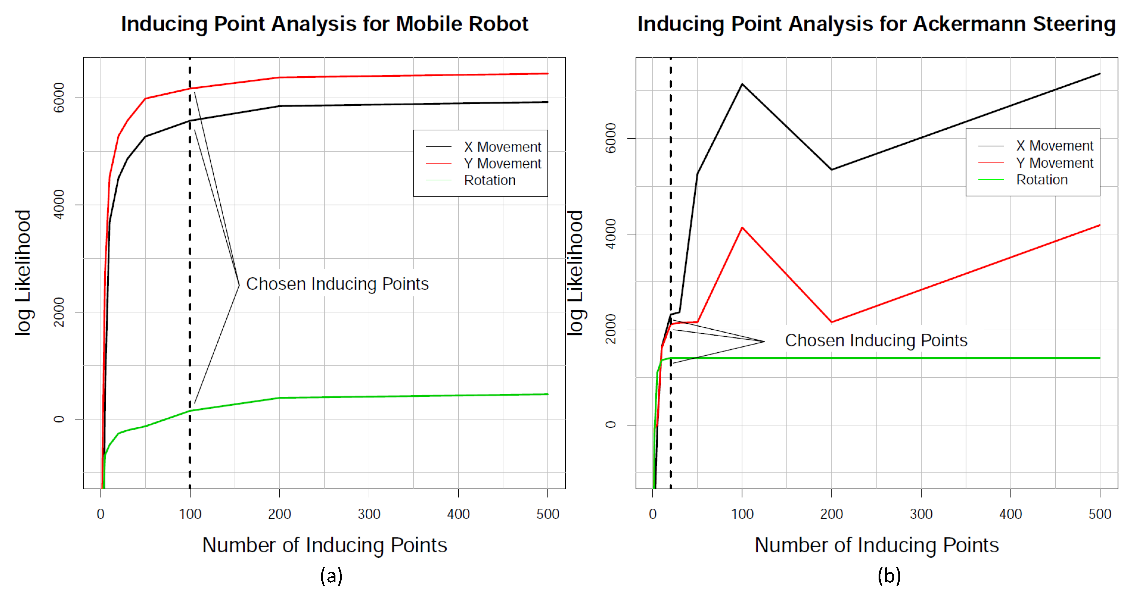
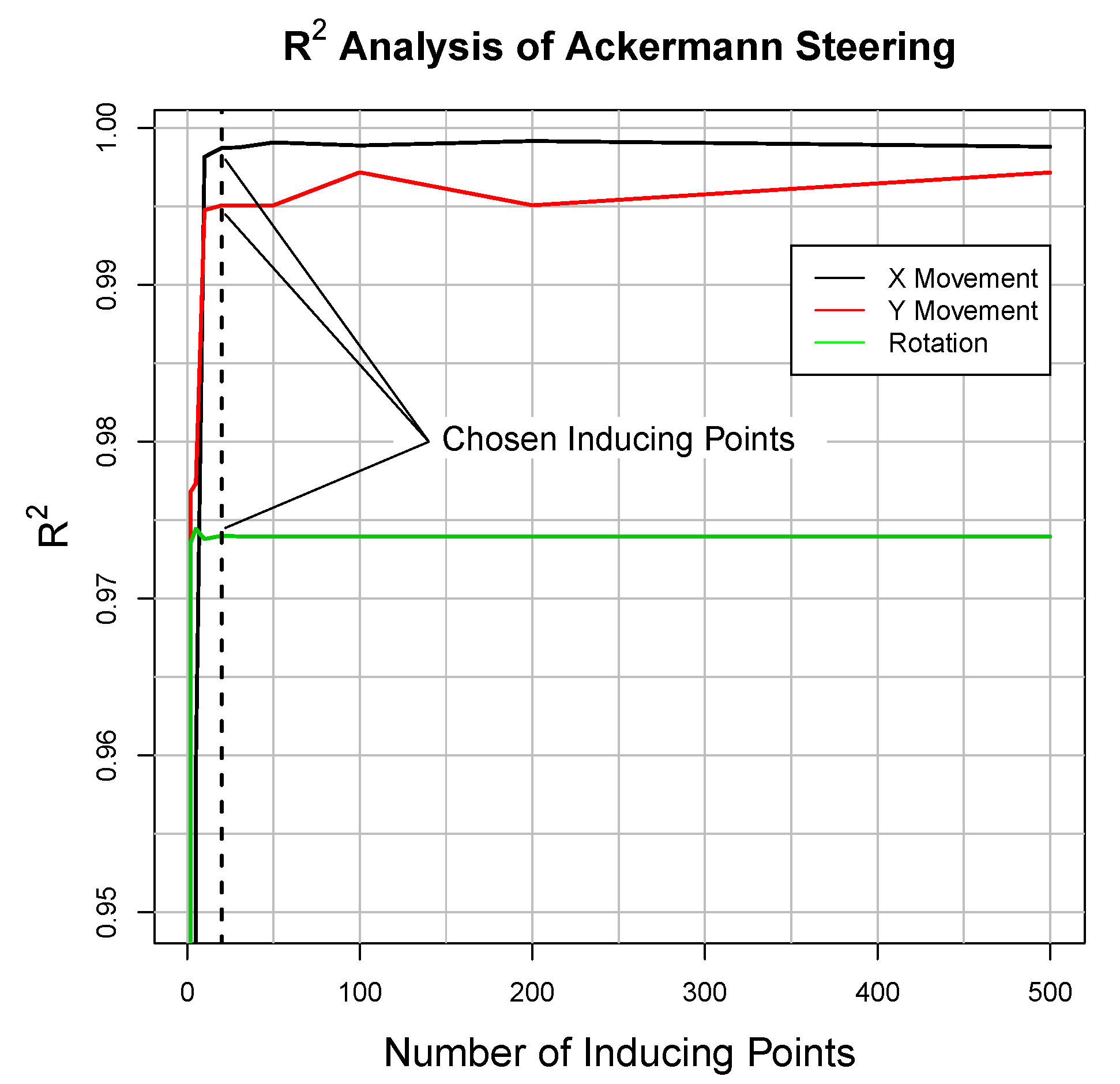
3.1. SGP Model Training

To train the motion in the sGP models a dataset is used that is based on the following Equation (6).

$$\mathcal{D}=\left\{\begin{array}{c}\left[\begin{array}{c}{\left(\begin{array}{c}\Delta {\varphi }_1\\ \cdots \\ \Delta {\varphi }_m\\ \theta \end{array}\right)}_0,{\left(\begin{array}{c}\Delta x\\ \Delta y\\ \Delta \theta \end{array}\right)}_0\end{array}\right],\cdots ,\left[\begin{array}{c}{\left(\begin{array}{c}\Delta {\varphi }_1\\ \cdots \\ \Delta {\varphi }_m\\ \theta \end{array}\right)}_n,{\left(\begin{array}{c}\Delta x\\ \Delta y\\ \Delta \theta \end{array}\right)}_n\end{array}\right]\end{array}\right\}.$$

(6)

We then estimate the vehicle parameters for a differential driven mobile robot and a car. The kinematic models used for this calculation are depicted in Figure 4 and described in [45]. Note that we use a virtual wheel for the Ackermann kinematics. This approach is similar to the bicycle simplification described in [46].

Both models use the instantaneous center of rotation (ICR), sometimes known as instantaneous center of curvature (ICC).

The movement of the mobile robot refers to the center of the baseline P. The kinematic model is described using the vehicle parameters $\overline{r}$ (mean wheel radius) and B (distance between wheels), the simulated ground truth data and wheel movement $\Delta {\varphi }_{t,\{r,l\}}$ at time t as denoted in Equation (7):

$${\left(\begin{array}{c}\Delta x\\ \Delta y\\ \Delta \theta \end{array}\right)}_t=\left(\begin{array}{c}\frac{(\Delta {\varphi }_{t,r}+\Delta {\varphi }_{t,l})·\overline{r}}{2}·\cos ({\theta }_{t-1}+\Delta {\theta }_{t-1})\\ \frac{(\Delta {\varphi }_{t,r}+\Delta {\varphi }_{t,l})·\overline{r}}{2}·\sin ({\theta }_{t-1}+\Delta {\theta }_{t-1})\\ \frac{(\Delta {\varphi }_{t,r}-\Delta {\varphi }_{t,l})·\overline{r}}{b}\end{array}\right).$$

(7)

Note that this representation is similar to the data set that we used for the sGP formulation in Equation (6).

To develop our model for evaluation we relied on the approach described in [43] and implemented in [47]. The parameter estimation and data pre-processing was done in R. We divided the data into $25\%$ for training and $75\%$ for testing. For each element in the state vector ${\overrightarrow{x}}_t={\left(\begin{array}{ccc}{x}_t& y_t& {\theta }_t\end{array}\right)}^T$, we trained an sGP model using an RBF kernel without automatic relevance determination. We estimated the models for the following $\{1,2,5,10,20,30,50,100,200,500\}$ auxiliary points. For each model, we analyzed the log likelihood $log\left(p\right(\mathbf{X}\left)\right)=\mathcal{L}\left(q\right)+KL\left(q\right|\left|p\right)$ [35]. $\mathcal{L}\left(q\right)$ is known as the lower bound and $KL\left(q\right|\left|p\right)$ is the Kullback–Leibler divergence [35]. We selected the number of auxiliary points when the model seemed to be converged.

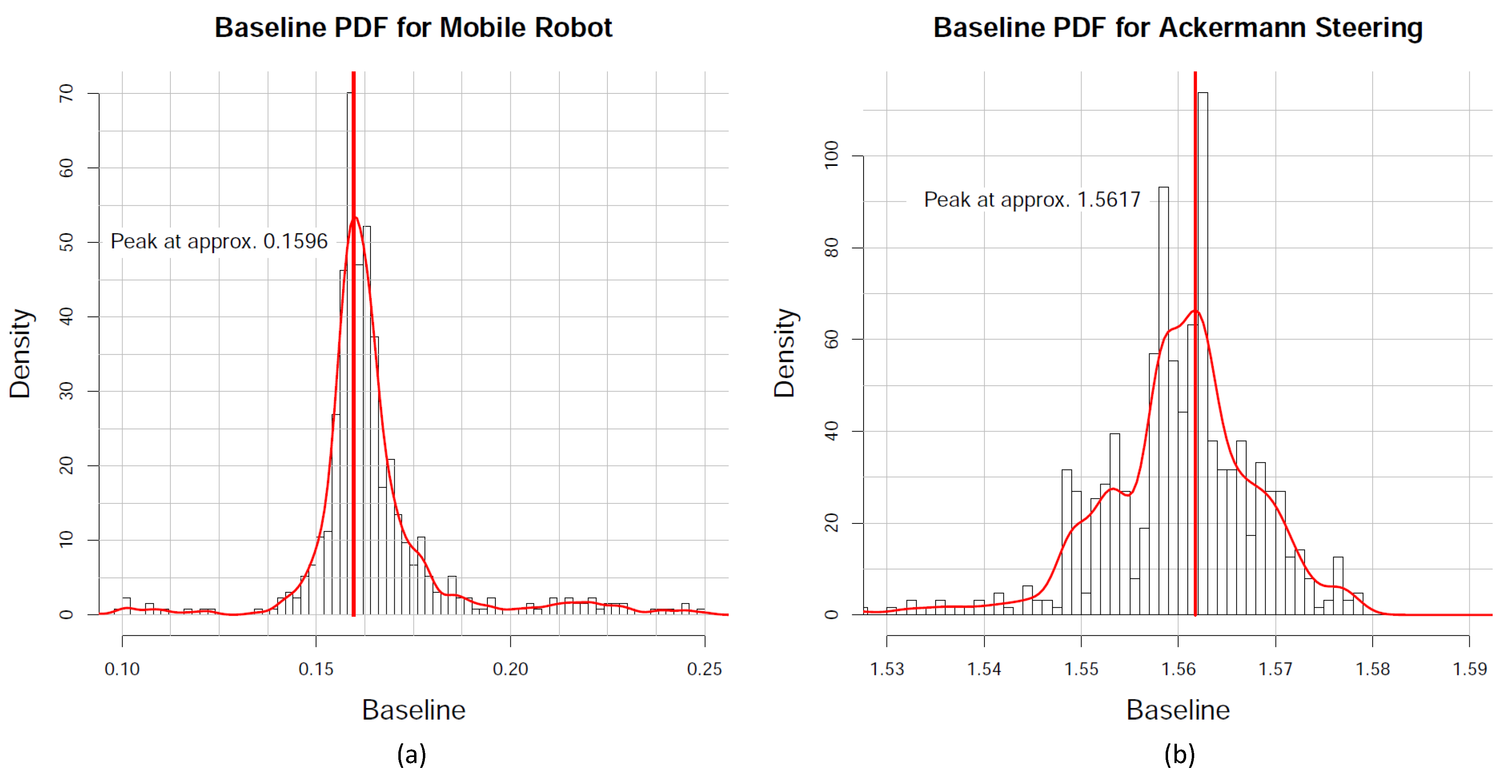
3.2. Vehicle Parameter Estimation

Throughout this paper a few assumptions have been made to derive the explanatory factors from the GP models, namely the car consists of a rigid body construction, the constant speed of the Ackerman vehicle and the sliding and rolling constraints. Where the rigid body assumption is one of the fundamental theories for kinematic models, which were used for wheel radii and distance estimation. Since physical characteristics of the vehicle must be described, this assumption has to be made.

The speed of the car was set to a constant speed for the purpose of simplicity to generate data. Since this assumption was not done in mobile robot experiments, we do not assume that variance in speed effects the parameter estimation. Finally, the sliding and rolling constraints are used to derive the kinematic equations which are the fundamental building stone of the GP algorithm.

Initially, we estimate $\overline{r}$ by rearranging Equation (8).

$$\rho =\sqrt{\Delta X^2+\Delta {\mathrm{Y}}^2}=\frac{(\Delta {\varphi }_{t,r}+\Delta {\varphi }_{t,l})·\overline{r}}{2}.$$

(8)

The baseline is estimated using $\Delta \theta$ but it is affected by singularities that are related to a straight movement. As with the mobile robot kinematic, the car movement refers to the center of the rear baseline P. Thus, we can use the same procedure for back wheel radius and baseline estimation. The radius of the virtual front wheel ${\overline{r}}_v$ can be calculated easily using the wheel movement. Finally, T (distance between front and rear axles) is determined using the ICR and basic kinematics, where we assume a stiff chassis and wheel motion. This estimation is done using R (distance/radius to ICR) and the baseline B.

In the approach presented in this paper we used a simulation set up that included noise for both vehicle models. Therefore we had to face multiple challenges, including difficulty estimating the baseline values for both models in a straightforward maneuver. This is due to the fact that the $\Delta \theta$ becomes zero, and unrealistically large baselines arise due to computational problems. Based on this and due to the fact that the distance to the ICR is significantly affected by noise, we assume a noisy and hard to estimate T. Furthermore, we currently use a point estimate of B and the mean wheel radii. Since we do not assume a Gaussian distribution for B, this will disturb the T calculation.

For mean wheel radius $\overline{r}$ estimation of the mobile robot, we performed a single prediction for $G{P}_x$, $G{P}_y$ and $G{P}_{\theta }$ using the mean value of the input (wheel movement $\Delta {\varphi }_{r,l}$). The sGP models estimate the inherent $\Delta X$, $\Delta \mathrm{Y}$ and $\Delta \theta$. Since both $\Delta X$ and $\Delta \mathrm{Y}$ are normally distributed according to sGP prediction and $\Delta {\varphi }_{r,l}$ are constants, we assume that $\overline{r}$ is also Gaussian.

Due to singularities for the baseline estimation (see $\Delta \theta$ calculation in Equation (7)), we used the whole test dataset of the sGP prediction. We excluded the motion data that fulfilled $(\Delta {\varphi }_r-\Delta {\varphi }_l)<0.1\left[rad\right]$ to exclude straightforward movement. We also deleted unrealistic baseline values by excluding estimated baselines that were smaller than 5 cm and larger than 0.5 m, where the ground truth is 16 cm.

For each resulting motion, we estimated a possible baseline length. We applied a histogram-based approach including kernel density estimation [48] to estimate the baseline value. For Ackermann steering, we followed the same procedure for the estimation of both the rear wheel radius ${\overline{r}}_b$ and the baseline B. We applied additional data filtering for faulty time stamps, where samples with a time differences above 0.1 seconds were deleted. As in the process applied with the mobile robot, we filtered the estimated baselines excluding the data for the motion of the rear wheels, in which $(\Delta {\varphi }_r-\Delta {\varphi }_l)<0.1\left[rad\right]$, describing $\Delta {\varphi }_{b,r}$ and $\Delta {\varphi }_{b,l}$ the rear wheel movement. Additionally, we removed unrealistic baselines that ranged above $110\%$ and below $90\%$ of the baseline median. Due to a higher noise level in the baseline values, absolute thresholding was not applicable.

For the virtual front wheel radii estimation, we used test input data from the simulation, having previously defined a driving scenario with a straight road so that the back wheels and front wheels could rotate in a comparable manner similarly to the virtual front wheel. Based on this we defined the following Equations (9) and (10).

$$\begin{array}{c}\hfill \Delta {\varphi }_v{r}_v=\frac{(\Delta {\varphi }_{f,r}+\Delta {\varphi }_{f,l})·{\overline{r}}_f}{2}=\rho =\frac{(\Delta {\varphi }_r+\Delta {\varphi }_l)·{\overline{r}}_b}{2}\end{array}$$

(9)

$$\begin{array}{c}\hfill r_v=\frac{(\Delta {\varphi }_r+\Delta {\varphi }_l)·{\overline{r}}_b}{2\Delta {\varphi }_v}=\frac{(\Delta {\varphi }_r+\Delta {\varphi }_l)·{\overline{r}}_b}{2\frac{(\Delta {\varphi }_{f,r}+\Delta {\varphi }_{f,l})}{2}}\sim \mathcal{N}\end{array}$$

(10)

in which we used the rear wheel movement $\Delta {\varphi }_{r,l}$, the front wheel movement $\Delta {\varphi }_{f,l}$ and $\Delta {\varphi }_{f,r}$ including the front wheel radius ${\overline{r}}_f$ and the estimated rear wheel radius ${\overline{r}}_b\sim \mathcal{N}$. Note that the front and rear wheel mean radii are not equal. For each element in the test input, we performed the radii estimation for the radius from Equation (10). The resulting set of Gaussian distributions are combined using the basic properties of Gaussian distributions.

Since the sGP models estimate the movement of the vehicle for P, the complete description of the rear kinematics of the Ackermann steering is enough to estimate the vehicle’s behavior. Since the kinematic constraints connect the virtual wheels and rear wheels through the ICR, we could implement a motion model for a Bayes filter without estimating T. This is different to the bicycle model described in [46], where the kinematic model is reduced to a virtual rear as well as a front wheel. Since all the motion parameters refer to the center of the rear baseline value, we can estimate $\Delta X$, $\Delta \mathrm{Y}$ and $\Delta \theta$ without T. However, we estimate T in order to have a more complete insight into the models. We calculated T using the test wheel motion, estimated baseline B and the distance R to the ICR. We estimated T through ${\overrightarrow{v}}_t={\overrightarrow{\omega }}_t\times \overrightarrow{k}$, where $\overrightarrow{k}$ describes distances and includes T. This calculation includes the factor $\frac{{\overline{r}}_b}{r_v}$.

3.3. Comparison of the Presented Approach with Blackbox and Whitebox Models

To compare the presented methodology to blackbox and whitebox models we implemented the movement model $p\left({\overrightarrow{x}}_t\right|{\overrightarrow{x}}_{t-1},{\overrightarrow{u}}_t)$ with additional approaches.

We selected as blackbox models Bayesian neuronal networks and defined a single hidden layer and output neurons for X, Y and $\theta$. Fifteen hidden neurons and 60 epochs were used for mobile robot experiments. This architecture results in 204 trainable parameters. For Ackermann steering, 40 hidden neurons and 200 epochs were used. Five hundred and twenty-nine trainable parameters were used to implement this architecture. Both models were implemented in Tensorflow Probability, an extension of Tensorflow for probabilistic deep learning.

To compare the presented methodology to whitebox models, Bayesian linear regression was implemented. The Bayesian linear regression model was implemented in [49].

4. Results

As previously mentioned, we evaluated the proposed approach in a laboratory-controlled environment using a simulator framework that included a differential drive mobile robot and an Ackermann steered vehicle.

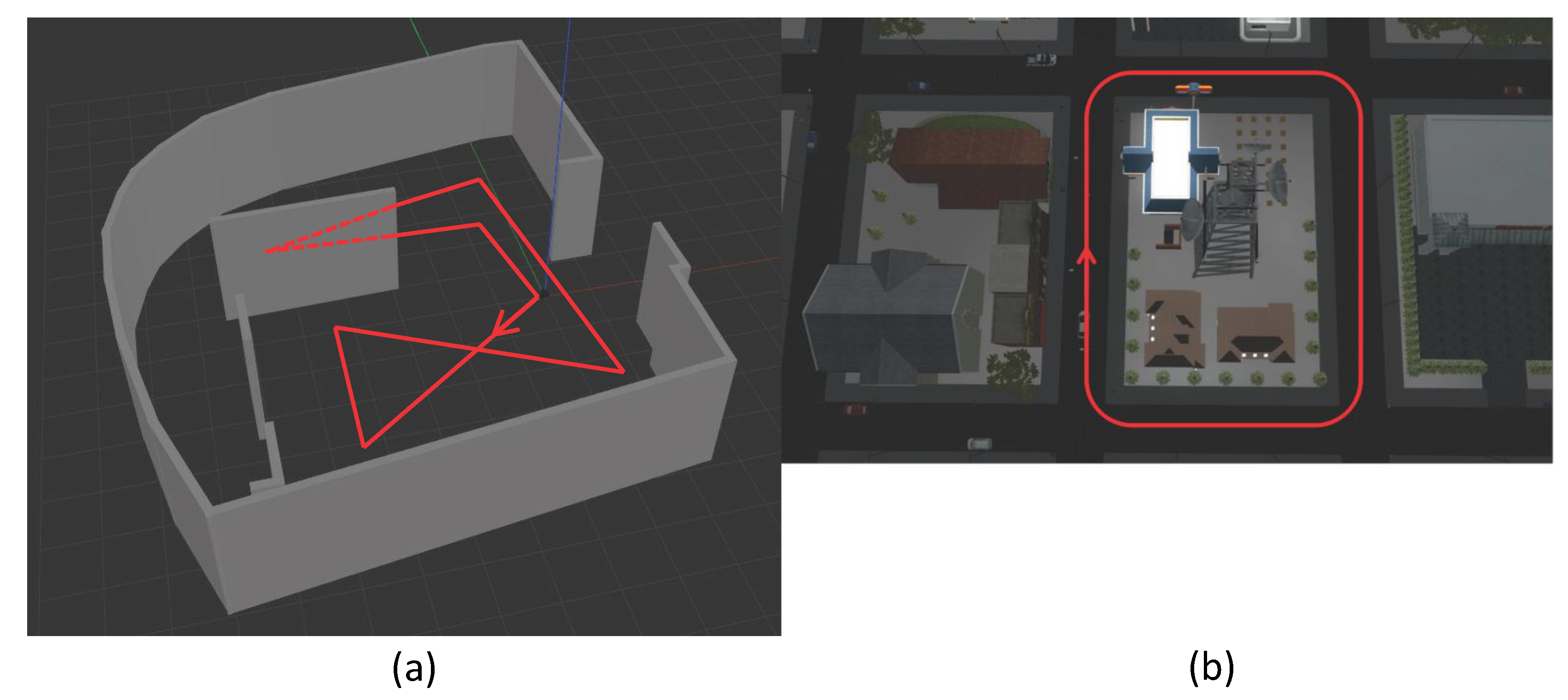
4.1. Ground Truth Data Generation

For the mobile robot simulation we used a Turtlebot version 3 model (See: https://www.turtlebot.com/) integrated in a ROS-Gazebo [50] (See: http://gazebosim.org/tutorials?tut=ros_overview) simulation. This mobile robot is based on a differential drive setup consisting of wheels with a radius of 3.3 cm and a baseline of 16 cm. We simulated a mobile robot task where the autonomous vehicle moves between stations in a factory or storage depot as a potential use case for transport logistics. To this end we used the test factory model described in [51]. The model for our use case is depicted in Figure 5a.

The Ackermann steering simulation was based on a model of a Toyota Prius (See: https://github.com/osrf/car_demo) integrated in a ROS-Gazebo simulation. With this model we carried out simulations with the baseline of 1.586 m and the distance between the front and back wheels of 2.860 m (T). The wheel radii were set to 31.265 cm. The environment and test track is shown in Figure 5b. Both of these simulation setups provide simulated ground truth data (See: http://docs.ros.org/electric/api/gazebo_plugins/html/group__GazeboRosP3D.html) ($x,y,\theta$) as well as the rotation of the wheel joints (See: http://wiki.ros.org/joint_state_controller) of the vehicular robots. Further, since the focus of our work is on vehicle parameter estimation rather than autonomous vehicle control, other road users, such as pedestrians or other cars, where not included in the simulation.

Furthermore, we would like to state that the linear velocity of the Ackermann simulation is constant except for the initial acceleration. The mobile robot was controlled using the ROS navigation stack. (See: http://wiki.ros.org/navigation).

4.2. Motion Model and Vehicle Parameter Estimation

For the purpose of this study, our experiments are divided into two parts:

• Motion Model: We need to fit the sGP motion model to the data. In doing so, we need to optimize parameters and to ensure that the model represents the simulated movement.
• Kinematic Parameter Estimation: The kinematic parameter estimation is based on the result of the motion model and simplified vehicle kinematics.

The result of the sGP modelling is shown in Figure 6a for the mobile robot and Figure 6b for Ackermann steering. Based on the methodology proposed in [43], we chose the number of inducing points visually. This is in contrast to VB applications such as [52], where a marginal likelihood maximum occurs. One hundred auxiliary variables were determined, which were used by the model to create 100 pseudo vehicle movements and thereby estimate overall robot behavior.

The Ackermann steering model log likelihood for $G{P}_x$ and $G{P}_y$ increases significantly after initial convergence. Due to the $R^2$ analyzis of the test data, we assume that 20 auxiliary variables are sufficient to represent the physical system (see Figure 6b). The $R^2$ analyzis is shown in Figure 7. Since there is no significant improvement after 20 auxiliary points, we chose this configuration.

Based on Equation (8), we defined the probability density function of the mobile robot and Ackermann steering wheel radii (see Equations (11) and (12)).

$$\begin{array}{cc}\hfill \mathrm{Mobile} \mathrm{robot} \mathrm{wheel} \mathrm{radii}:& \overline{r}\sim \mathcal{N}({\mu }_r,{\sigma }_r^2)=\mathcal{N}(0.03329,1.327\times {10}^{-8})\hfill \end{array}$$

(11)

$$\begin{array}{cc}\hfill \mathrm{Ackermann} \mathrm{steering} \mathrm{read} \mathrm{wheel} \mathrm{radii}:& {\overline{r}}_b\sim \mathcal{N}({\mu }_r,{\sigma }_r^2)=\mathcal{N}(0.30797,2.680\times {10}^{-5})\hfill \end{array}$$

(12)

In both cases, the uncertainty (variance) is low. We assume that uncertainty will increase in real applications. The mobile robot simulation is based on a real wheel radius of 0.033 m (See http://wiki.ros.org/turtlebot3) for robot simulation details, and therefore the error is ∼2.7 % or 0.029 mm. Similar to that, the simulated ground truth of the Ackermann steering simulation is 0.31265 m (see Section 4.1), leading to an error of ∼5.6 % or 0.46 mm.

The baseline histogram and kernel density estimation of the filtered baseline values B for both models is shown in Figure 8. For the mobile robot simulation, the peak of the kernel density estimation is at approximately 0.1596 m, the simulation being based on the baseline of 0.16 m (see Section 4.2). This is an error of 0.25 % or 0.04 mm. Similar to that, the baseline value for the Ackermann steering was estimated at 1.5616 m, resulting in an error of ∼1.5 % or 2.4 cm. The simulated ground truth is 1.586 (see Section 4.1).

Additionally, the estimation of the virtual front wheel probability density function $r_v$ resulted in the same probability density function as the mean rear wheel radii ${\overline{r}}_b$ (see Equation (13))

$$r_v\sim \mathcal{N}({\mu }_r,{\sigma }_r^2)=\mathcal{N}(0.30797,2.680\times {10}^{-5}).$$

(13)

We assumed that the radii are equal and thus slipping and rolling constraints apply to motion.

Finally, the estimated T values are depicted in Figure 9. We estimated the peak of the kernel density at ∼2.7579 m, the simulated ground truth measuring 2.86 m (see Section 4.1). It results in an error of ∼3.5% or 10.21 cm. The estimated parameters, including simulated ground truth values, are summarized in

Table 1. Summarized results of derived vehicle parameters from the sGP motion models (M) and simulated ground truth (GT).

	${\overline{\mathit{r}}}_{\left(\mathit{b}\right)}$		B		${\overline{\mathit{r}}}_{\mathit{v}}$		T
	M	GT	M	GT	M	GT	M	GT
Mobile Robot	3.329 cm	3.300 cm	15.96 cm	16 cm	-	-	-	-
Ackermann Steering	30.79 cm	31.26 cm	1.561 m	1.586 m	30.797 cm	31.265 cm	2.757 m	2.86 m

.

To analyse real-time capability of the presented methodology, time measurements for sGP prediction were done. For 100 inducing points of the mobile robot model, 15.425 ms were measured for a single prediction. For Ackermann steering, 0.284 ms were measured for the 20 inducing point model. Both experiments were performed on an Intel i9-7900X CPU. However, the used sGP implementation [47] is a CPU implementation. Similar to GPU optimized software for artificial neuronal networks such as [53], software for GPU based GP acceleration is under development [54].

We performed additional simulation for the Ackermann kinematic model using different wheel radii for front and rear. Furthermore, we changed the friction coefficient. We used 20 inducing points for the simulations AM2 and AM3 and 200 inducing points for the simulation AM1 (we chose a friction coefficient for rubber and wet concrete based on https://hypertextbook.com/facts/2006/MatthewMichaels.shtml). The results are summarized in

Table 2. Summarized results additional simulation results for Ackermann (AM) steering. AM 1 and AM 2 are based on the standard friction of $0.9$ for dry concrete. For AM 3, we changed the friction coefficient to $0.45$. The histograms for AM 1–AM 3 can be found in the Supplementary Materials.

	${\overline{\mathit{r}}}_{\left(\mathit{b}\right)}$		B		${\overline{\mathit{r}}}_{\mathit{v}}$		T
	M	GT	M	GT	M	GT	M	GT
AM 1	26.890 cm	26.265 cm	1.629 m	1.586 m	35.428 cm	36.270 cm	2.522 m	2.860 m
AM 2	29.105 cm	30.000 cm	1.534 m	1.586 m	23.142 cm	25.000 cm	2.437 m	2.860 m
AM 3	29.872 cm	30.000 cm	1.581 m	1.586 m	26.890 cm	25.000 cm	2.443 m	2.860 m

.

The results based on additional simulation show, that the presented methodology is able to estimate vehicle parameters with different front and read wheel radii. Similar to the initial results (see Table 1), our approach estimates T not as accurate as the wheel radii and B.

4.3. Comparison of Whitebox and Blackbox Models

The presented work based on sGP models was compared to whitebox (Bayesian linear regression) and blackbox (Bayesian artificial neuronal networks) models. Results from this comparison of the Bayesian neuronal networks are summarized in

Table 3. Summarized results based on the blackbox model Bayesian neuronal networks of vehicle parameters from the sGP motion models (M) and simulated ground truth (GT). For mobile robot experiments, 15 hidden neurons were used in the hidden layer. For Ackermann steering experiments, 40 hidden neurons were used.

	${\overline{\mathit{r}}}_{\left(\mathit{b}\right)}$		B		${\overline{\mathit{r}}}_{\mathit{v}}$		T
	M	GT	M	GT	M	GT	M	GT
Mobile Robot	3.683 cm	3.300 cm	17.866 cm	16 cm	-	-	-	-
Ackermann Steering	28.429 cm	31.26 cm	1.436 m	1.586 m	28.429 cm	31.265 cm	2.582 m	2.86 m

.

The Bayesian neuronal network performs inferior to the sGP methodology.

As for the whitebox model example through Bayesian linear regression, the data was analysed using $R^2$ values. For mobile robot movement, $R^2$ values of $0.168$ for X, $0.735$ for Y and $0.884$ for $\theta$ were estimated. $R^2$ values of $0.445$ for X, $0.423$ for Y and $0.982$ for $\theta$ for the Ackermann steered vehicle were estimated. Due to the low $R^2$ values, no parameter estimation was performed.

5. Conclusion and Future Work

We rejected the Null hypothesis and accept therefore the alternative hypothesis:

H1: 

sGP-based motion models are able to learn movement based on wheel motion.

By converting blackbox motion models to models that describe the model behavior using vehicle kinematics. For the implementation, we chose a sGP-based modelling approach, where we modeled $p\left({\overrightarrow{x}}_t\right|{\overrightarrow{x}}_{t-1},{\overrightarrow{u}}_t)$ using wheel motion as command input ${\overrightarrow{u}}_t$. Since the input to our parameter estimation is wheel motion and Gaussian distributed motion (see Equations (8) and (10)), any model can be used to produce these data. We selected sGP instead of other models, such as Bayesian neuronal networks [22], due to the non-parametric nature of the defined problem, which decreases user-based bias. Nevertheless, experiments using Bayesian neuronal networks (blackbox model) and Bayesian linear regression (whitebox model) were performed. Both models performed inferior in comparison to sGP models.

For sGP motion models, we used the lower bound and Kullback–Leibler divergence to derive the number of auxiliary points for the GP approximation. This approach results in a probabilistic motion model for vehicle behavior. To get insight into the blackbox motion model, we simulated vehicle movement starting from a known position. This movement was used to parameterize the kinematic model, where we used basic properties of probability density functions and kernel density estimation to calculate the vehicle parameters. Using minor additional physical assumptions, we estimated the vehicle’s (rear) wheel radii and (read) baseline. It is possible to estimate those parameters between 0.25% and 5.6% prediction accuracy. Our additional simulation results showed that our methodology can estimate vehicle parameters with different front and rear wheel radii. Using additional assumptions, namely possible ICR positions and reasonable values, we estimated a T value close to the simulated ground truth.

The results show, that the sGP based motion model is able to learn movement based on wheel motion, being thus able to reject the null hypothesis. The presented methodology proves, that the sGP learns vehicle parameters implicitly. In contrast to that, the major shortcoming of sGP models is the limited real-time applicability. Our results show, that sGP models still has real-time issues and the real-time capability strongly depends on the number of auxiliary points. However, novel software packages such as [54] may solve this shortcoming by GPU acceleration.

We assume that real movement data will result in significantly higher variance values. Therefore, future work will address the analysis of real vehicle data as opposed to simulated models and also the evaluation of the derived motion model compared to classic physics-based models as well as dynamical models. The assumptions defined in this study, namely the rigid body assumption and rolling/sliding constraints, were used to derive the vehicle parameters from the sGP models. For real vehicles, those assumptions are typically violated on a small level between the timeslots t and $t+1$. This violation results in additional movement noise. However, as long as this violation is random, the applicability of the presented methodology to real data is not restricted. We do not assume systematic errors based on the assumptions during low speed maneuver. Furthermore, the presented methodology currently assumes equal wheel radii in front and rear. This limits the applicability to vehicles, where similar wheels are used and the mean radii is a reasonable approximation.

Additionally to noise introduced by assumption violation, real sensor signals can also introduce noise to the sGP estimation and thus to the vehicle parameter estimation. We assume that this noise will increase the estimation uncertainty but not the expected values as long as the disturbances are random and not systematic. Furthermore, since we can already describe the vehicle parameters in the graphical model of the Bayes filter, we will use VB approaches to derive the vehicle parameters in future work instead of relying on kinematic-based approaches to automate the process of parameters estimation.

Finally, future work will also integrate other kinematic models (e.g., four wheel drive or mecanum wheels) state-of-the-art motion models such as deep GP [33] and the integration of the estimated vehicle parameter probability density functions to a localization approach. Afterwards we will be able to compare our localization approach to existing methodologies.

References

1. Thrun, S.; Burgard, W.; Fox, D. Probabilistic Robotics; MIT Press: Cambridge, MA, USA, 2006. [Google Scholar]
2. Dictionary, O.E. Definition of Vehicle. Available online: https://www.dictionary.com/browse/vehicle (accessed on 9 September 2020).
3. Dictionary, O.E. Definition of Robot. Available online: https://www.dictionary.com/browse/robot (accessed on 9 September 2020).
4. Pendleton, S.D.; Andersen, H.; Du, X.; Shen, X.; Meghjani, M.; Eng, Y.H.; Rus, D.; Ang, M.H. Perception, planning, control, and coordination for autonomous vehicles. Machines 2017, 5, 6. [Google Scholar] [CrossRef]
5. Li, J.; Dai, B.; Li, X.; Xu, X.; Liu, D. A dynamic bayesian network for vehicle maneuver prediction in highway driving scenarios: Framework and verification. Electronics 2019, 8, 40. [Google Scholar] [CrossRef] [Green Version]
6. da Costa Botelho, S.S.; Drews, P.; Oliveira, G.L.; da Silva Figueiredo, M. Visual odometry and mapping for underwater autonomous vehicles. In Proceedings of the 2009 6th Latin American Robotics Symposium (LARS 2009), Valparaiso, Chile, 29–30 October 2009; IEEE: Piscataway, NJ, USA, 2009; pp. 1–6. [Google Scholar]
7. Russell, S.; Norvig, P. Quantifying Uncertainty. In Artificial Intelligence: A Modern Approach, 3rd ed.; Prentice Hall: Upper Saddle River, NJ, USA, 2010. [Google Scholar]
8. Ko, J.; Fox, D. GP-BayesFilters: Bayesian Filtering Using Gaussian Process Prediction and Observation Models. In Proceedings of the IEEE/RSJ International Conference on Intelligent Robots and Systems (IROS), Nice, France, 22–26 September 2008; IEEE: Nice, France, 2008. [Google Scholar]
9. Fox, D. KLD-Sampling: Adaptive Particle Filters and Mobile Robot Localization. In Proceedings of the Advances in Neural Information Processing Systems (NIPS), Vancouver, BC, Canada, 3–8 December 2001. [Google Scholar]
10. Pearl, J. Causality: Models, Reasoning and Inference, 2nd ed.; Cambridge University Press: New York, NY, USA, 2009. [Google Scholar]
11. Pearl, J. Probabilistic Reasoning in Intelligent Systems: Networks of Plausible Inference; Morgan Kaufmann Publishers Inc.: San Francisco, CA, USA, 1988. [Google Scholar]
12. Bishop, C.M. Sequential Data. In Pattern Recognition and Machine Learning; Springer: New York, NY, USA, 2006. [Google Scholar]
13. Russell, S.; Norvig, P. Probabilistic Reasoning Over Time. In Artificial Intelligence: A Modern Approach, 3rd ed.; Prentice Hall: Upper Saddle River, NJ, USA, 2010. [Google Scholar]
14. Larsen, T.D.; Hansen, K.L.; Andersen, N.A.; Ole, R. Design of Kalman filters for mobile robots; evaluation of the kinematic and odometric approach. In Proceedings of the 1999 IEEE International Conference on Control Applications (Cat. No.99CH36328), Kohala Coast, HI, USA, 22–27 August 1999; Volume 2, pp. 1021–1026. [Google Scholar]
15. Thrun, S.; Burgard, W.; Fox, D. Gaussin Filters. In Probabilistic Robotics; MIT Press: Cambridge, MA, USA, 2006. [Google Scholar]
16. Konstantin, A.; Kai, S.; Rong-zhong, L. Modification of Nonlinear Kalman Filter Using Self-organizing Approaches and Genetic Algorithms. Int. J. Inf. Eng. 2013, 3, 129–136. [Google Scholar]
17. Shakhtarin, B.I.; Shen, K.; Neusypin, K. Modification of the nonlinear kalman filter in a correction scheme of aircraft navigation systems. J. Commun. Technol. Electron. 2016, 61, 1252–1258. [Google Scholar] [CrossRef]
18. Shen, K.; Wang, M.; Fu, M.; Yang, Y.; Yin, Z. Observability Analysis and Adaptive Information Fusion for Integrated Navigation of Unmanned Ground Vehicles. IEEE Trans. Ind. Electron. 2020, 67, 7659–7668. [Google Scholar] [CrossRef]
19. Julier, S.J.; Uhlmann, J.K. New extension of the Kalman filter to nonlinear systems. In Signal Processing, Sensor Fusion, and Target Recognition VI; Kadar, I., Ed.; International Society for Optics and Photonics, SPIE: Bellingham, WA, USA, 1997; Volume 3068, pp. 182–193. [Google Scholar]
20. Pearl, J.; Mackenzie, D. The Book of Why: The New Science of Cause and Effect, 1st ed.; Basic Books, Inc.: New York, NY, USA, 2018. [Google Scholar]
21. Bengio, Y.; Courville, A.C.; Vincent, P. Unsupervised Feature Learning and Deep Learning: A Review and New Perspectives. arXiv 2012, arXiv:1206.5538. [Google Scholar]
22. Neal, R. Bayesian Learning for Neuronal Networks. Ph.D. Thesis, University of Toronto, Toronto, ON, Canada, 1995. [Google Scholar]
23. Hartikainen, J.; Särkkä, S. Kalman filtering and smoothing solutions to temporal Gaussian process regression models. In Proceedings of the 2010 IEEE International Workshop on Machine Learning for Signal Processing (MLSP), Espoo, Finland, 21–24 September 2020. [Google Scholar]
24. Reece, S.; Roberts, S. An introduction to Gaussian processes for the Kalman filter expert. In Proceedings of the 2010 13th Conference on Information Fusion (FUSION), Edinburgh, UK, 26–29 July 2010. [Google Scholar]
25. Rasmussen, C.E.; Williams, C.K.I. Gaussian Processes for Machine Learning (Adaptive Computation and Machine Learning); The MIT Press: Cambridge, MA, USA, 2005. [Google Scholar]
26. Bishop, C.M. Kernel Methods. In Pattern Recognition and Machine Learning; Springer: New York, NY, USA, 2006. [Google Scholar]
27. Lefèvre, S.; Vasquez, D.; Laugier, C. A survey on motion prediction and risk assessment for intelligent vehicles. ROBOMECH J. 2014, 1, 1. [Google Scholar] [CrossRef] [Green Version]
28. Paden, B.; Čáp, M.; Yong, S.Z.; Yershov, D.; Frazzoli, E. A survey of motion planning and control techniques for self-driving urban vehicles. IEEE Trans. Intell. Veh. 2016, 1, 33–55. [Google Scholar] [CrossRef] [Green Version]
29. Katrakazas, C.; Quddus, M.; Chen, W.H.; Deka, L. Real-time motion planning methods for autonomous on-road driving: State-of-the-art and future research directions. Transp. Res. Part C Emerg. Technol. 2015, 60, 416–442. [Google Scholar] [CrossRef]
30. Lundquist, C.; Karlsson, R.; Ozkan, E.; Gustafsson, F. Tire Radii Estimation Using a Marginalized Particle Filter. Intell. Transp. Syst. IEEE Trans. 2014, 15, 663–672. [Google Scholar] [CrossRef] [Green Version]
31. M’Sirdi, N.; Rabhi, A.; Fridman, L.; Davila, J.; Delanne, Y. Second order sliding mode observer for estimation of velocities, wheel sleep, radius and stiffness. Am. Control. Conf. 2006, 2006, 6. [Google Scholar] [CrossRef]
32. Zeiler, M.D.; Fergus, R. Visualizing and Understanding Convolutional Networks. arXiv 2013, arXiv:1311.2901. [Google Scholar]
33. Damianou, A.; Lawrence, N. Deep Gaussian Processes. In Proceedings of the Sixteenth International Conference on Artificial Intelligence and Statistics, San Diego, CA, USA, 9–12 May 2015; Carvalho, C.M., Ravikumar, P., Eds.; PMLR: Scottsdale, AZ, USA, 2013; Volume 31, pp. 207–215. [Google Scholar]
34. Titsias, M.K.; Lawrence, N.D. Bayesian Gaussian Process Latent Variable Model. In Proceedings of the Thirteenth International Conference on Artificial Intelligence and Statistics, AISTATS 2010, Chia Laguna Resort, Sardinia, Italy, 13–5 May 2010; pp. 844–851. [Google Scholar]
35. Blei, D.M.; Kucukelbir, A.; McAuliffe, J.D. Variational Inference: A Review for Statisticians. J. Am. Stat. Assoc. 2017, 112, 859–877. [Google Scholar] [CrossRef] [Green Version]
36. Wan, G.; Yang, X.; Cai, R.; Li, H.; Zhou, Y.; Wang, H.; Song, S. Robust and Precise Vehicle Localization Based on Multi-Sensor Fusion in Diverse City Scenes. In Proceedings of the 2018 IEEE International Conference on Robotics and Automation (ICRA), Brisbane, QLD, Australia, 21–25 May 2018; pp. 4670–4677. [Google Scholar] [CrossRef] [Green Version]
37. Yu, B.; Dong, L.; Xue, D.; Zhu, H.; Geng, X.; Huang, R.; Wang, J. A hybrid dead reckoning error correction scheme based on extended Kalman filter and map matching for vehicle self-localization. J. Intell. Transp. Syst. 2019, 23, 84–98. [Google Scholar] [CrossRef]
38. Kia, S.S.; Rounds, S.F.; Martínez, S. A centralized-equivalent decentralized implementation of Extended Kalman Filters for cooperative localization. In Proceedings of the 2014 IEEE/RSJ International Conference on Intelligent Robots and Systems, Chicago, IL, USA, 14–18 September 2014; pp. 3761–3766. [Google Scholar]
39. Jurevičius, R.; Marcinkevičius, V.; Šeibokas, J. Robust GNSS-denied localization for UAV using particle filter and visual odometry. Mach. Vis. Appl. 2019, 30, 1181–1190. [Google Scholar] [CrossRef] [Green Version]
40. Kim, H.; Liu, B.; Goh, C.Y.; Lee, S.; Myung, H. Robust Vehicle Localization Using Entropy-Weighted Particle Filter-based Data Fusion of Vertical and Road Intensity Information for a Large Scale Urban Area. IEEE Robot. Autom. Lett. 2017, 2, 1518–1524. [Google Scholar] [CrossRef]
41. Carvalho, H.; Moral, P.D.; Monin, A.; Salut, G. Optimal nonlinear filtering in GPS/INS integration. IEEE Trans. Aerosp. Electron. Syst. 1997, 33, 835–850. [Google Scholar] [CrossRef]
42. Seeger, M.; Williams, C.K.; Lawrence, N.D. Fast forward selection to speed up sparse Gaussian process regression. In Proceedings of the 9th International Workshop on Artificial Intelligence and Statistics, Key West, FL, USA, 3–6 January 2003. [Google Scholar]
43. Titsias, M.K. Variational Learning of Inducing Variables in Sparse Gaussian Processes. In Proceedings of the 12th International Conference on Artificial Intelligence and Statistics (AISTATS), Clearwater Beach, FL, USA, 16–18 April 2009. [Google Scholar]
44. Snelson, E.; Ghahramani, Z. Sparse Gaussian Processes using Pseudo-inputs. In Proceedings of the Advances in Neural Information Processing Systems (NIPS), Vancouver, BC, Canada, 5–8 December 2005. [Google Scholar]
45. Siegwart, R.; Nourbakhsh, I.R. Mobile Robot Kinematics. In Introduction to Autonomous Mobile Robots; Bradford Company: Holland, MI, USA, 2004. [Google Scholar]
46. Snider, J.M. Automatic Steering Methods for Autonomous Automobile Path Tracking; Tech. Rep.; Robotics Institute of Carnegie Mellon University: Pittsburgh, PA, USA, 2009. [Google Scholar]
47. GPy. GPy: A Gaussian Process Framework in Python. Since 2012. Available online: http://github.com/SheffieldML/GPy (accessed on 9 September 2020).
48. Bishop, C.M. Kernel Density Estimators. In Pattern Recognition and Machine Learning; Springer: New York, NY, USA, 2006. [Google Scholar]
49. Luttinen, J. BayesPy: Variational Bayesian Inference in Python. J. Mach. Learn. Res. 2016, 17, 1–6. [Google Scholar]
50. Koenig, N.; Howard, A. Design and use paradigms for gazebo, an open-source multi-robot simulator. In Proceedings of the 2004 IEEE/RSJ International Conference on Intelligent Robots and Systems (IROS) (IEEE Cat. No. 04CH37566), Sendai, Japan, 28 September–2 October 2004; Volume 3, pp. 2149–2154. [Google Scholar]
51. Otrebski, R.; Pospisil, D.; Engelhardt-Nowitzki, C.; Kryvinska, N.; Aburaia, M. Flexibility Enhancements in Digital Manufacturing by means of Ontological Data Modeling. Procedia Comput. Sci. 2019, 155, 296–302. [Google Scholar] [CrossRef]
52. Bishop, C.M. Determing the Number of Components. In Pattern Recognition and Machine Learning; Springer: New York, NY, USA, 2006. [Google Scholar]
53. Chollet, F. Keras. 2015. Available online: https://keras.io (accessed on 9 September 2020).
54. Matthews, A.G.D.G.; van der Wilk, M.; Nickson, T.; Fujii, K.; Boukouvalas, A.; León-Villagrá, P.; Ghahramani, Z.; Hensman, J. GPflow: A Gaussian process library using TensorFlow. J. Mach. Learn. Res. 2017, 18, 1–6. [Google Scholar]
Figure 1. Graphical probabilistic model describing the Bayes filter. Each node describes a random variable. x j describes the vehicle’s state at time j, z j describes a measurement and u j a control state. Note that due to readability, we skipped the vector arrow in the figure.
Applsci 10 06317 g001
Figure 2. Proposed approach of this study for vehicle parameter estimation. The on-board sensory systems measure the wheel movement ( Δ ϕ r and Δ ϕ l ). Based on simulated global vehicle poses (gray arrows), we derive hidden vehicle parameters ( Θ = ( r r , r l , B ) ).
Applsci 10 06317 g002
Figure 3. Graphical model including the vehicle parameters (a). Since we perform simulation from a known pose using the movement model, the connections to x t disappear (b).
Applsci 10 06317 g003
Figure 4. Visualization of the kinematic models used for the performed mobile robot (a) and car experiments (b). For both models, we assumed a rigid frame. For the car model, we used a simplified version of Ackermann steering using a virtual wheel. The doted lines are the zero-motion lines of the wheels and thus represent kinematic constrains of the wheels.
Applsci 10 06317 g004
Figure 5. Overview of the setup of the simulation environments, namely the test factory (a) and the car environment (b).
Applsci 10 06317 g005
Figure 6. Visualization of implemented sparsed Gaussian processe (sGP) models. We select 100 auxiliary points for the mobile robot (a). After analyzing the R 2 value of the Ackermann motion models, we chose 20 auxiliary points for the car simulation (b).
Applsci 10 06317 g006
Figure 7. Visualization of the R 2 values of the sGP model estimation.
Applsci 10 06317 g007
Figure 8. Baseline estimation for both kinematic models using kernel density estimation and maximum (red line). The used bin sizes are 0.002 m for mobile robot baseline (a) and 0.001 m for Ackermann steering (b).
Applsci 10 06317 g008
Figure 9. Estimation of T using the instantaneous center of rotation (ICR). The used bin size is 0.05 m.
Applsci 10 06317 g009