Optical Characterization of Homogeneous and Heterogeneous Intralipid-Based Samples


Abstract
1. Introduction
2. Light Propagation in Turbid Media
2.1. Static and Dynamic Light Scattering
2.2. Diffusion Approximation
2.2.1. Homogeneous Slab
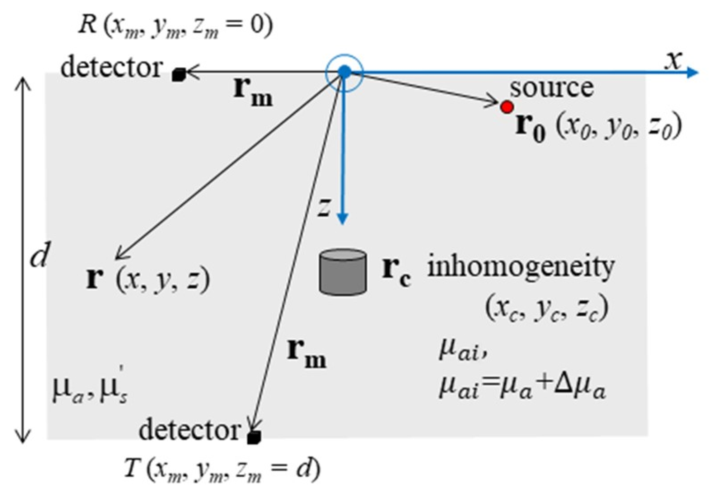
2.2.2. Heterogeneous Slab
3. Materials and Methods
3.1. Sample Preparation
3.1.1. Liquid Suspensions
3.1.2. Absorptive Cylindrical Inclusions
3.2. Experimental Techniques and Data Analysis Procedures
3.2.1. Static and Dynamic Light Scattering Experiments
3.2.2. Time-Resolved Transmittance Experiments
4. Results and Discussion
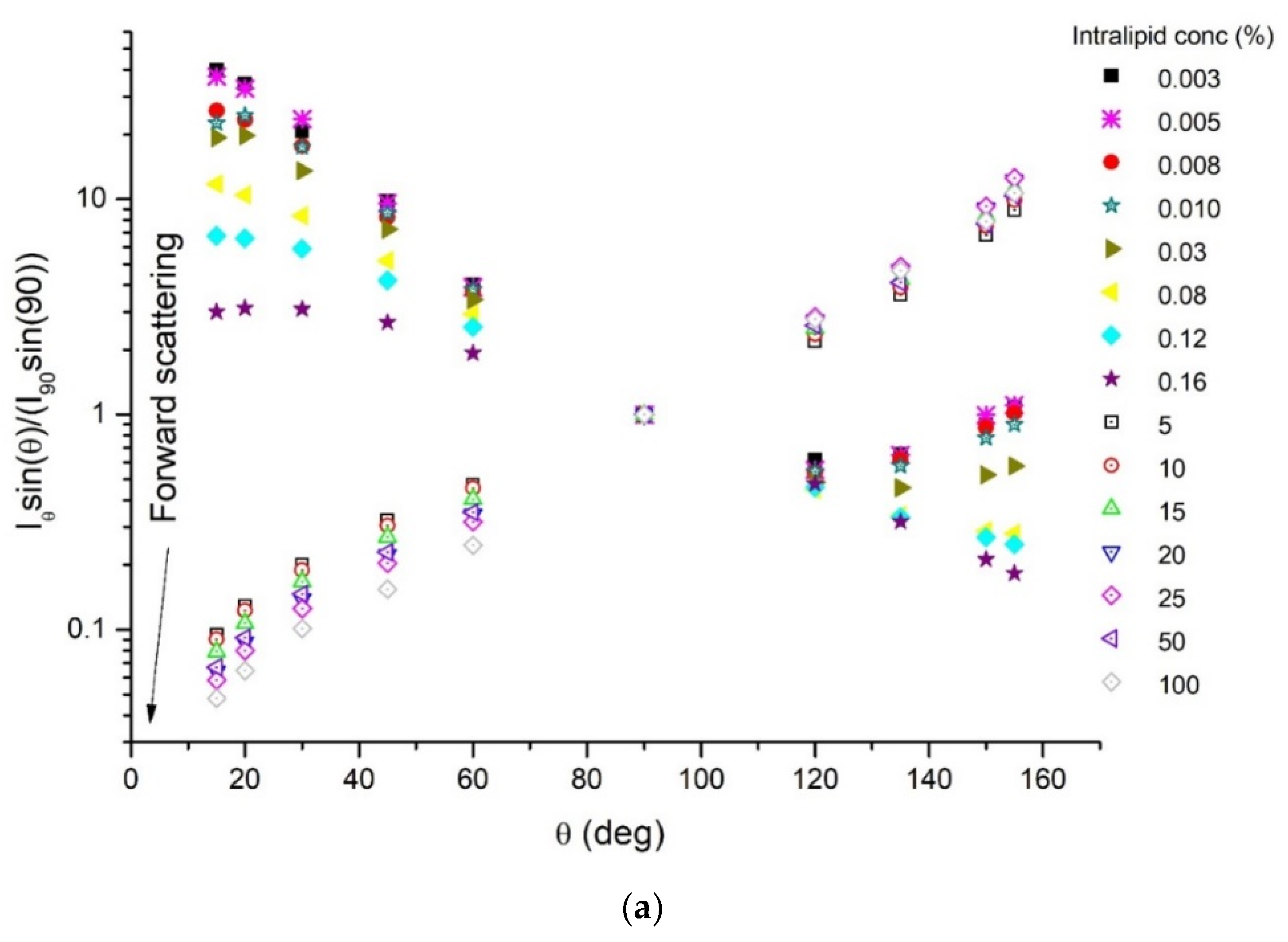
4.1. SLS Results
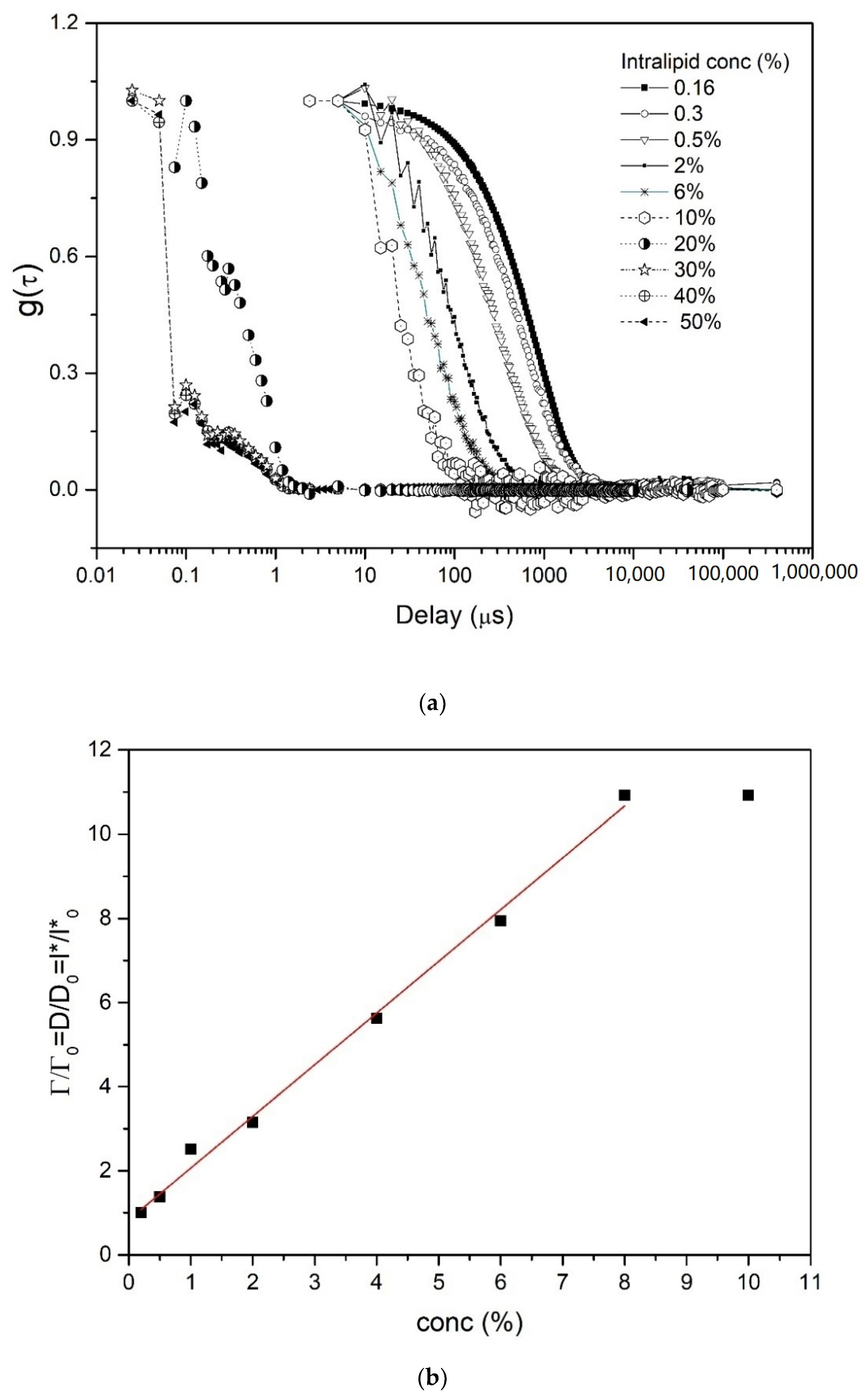
4.2. DLS Results
4.3. TRT Results
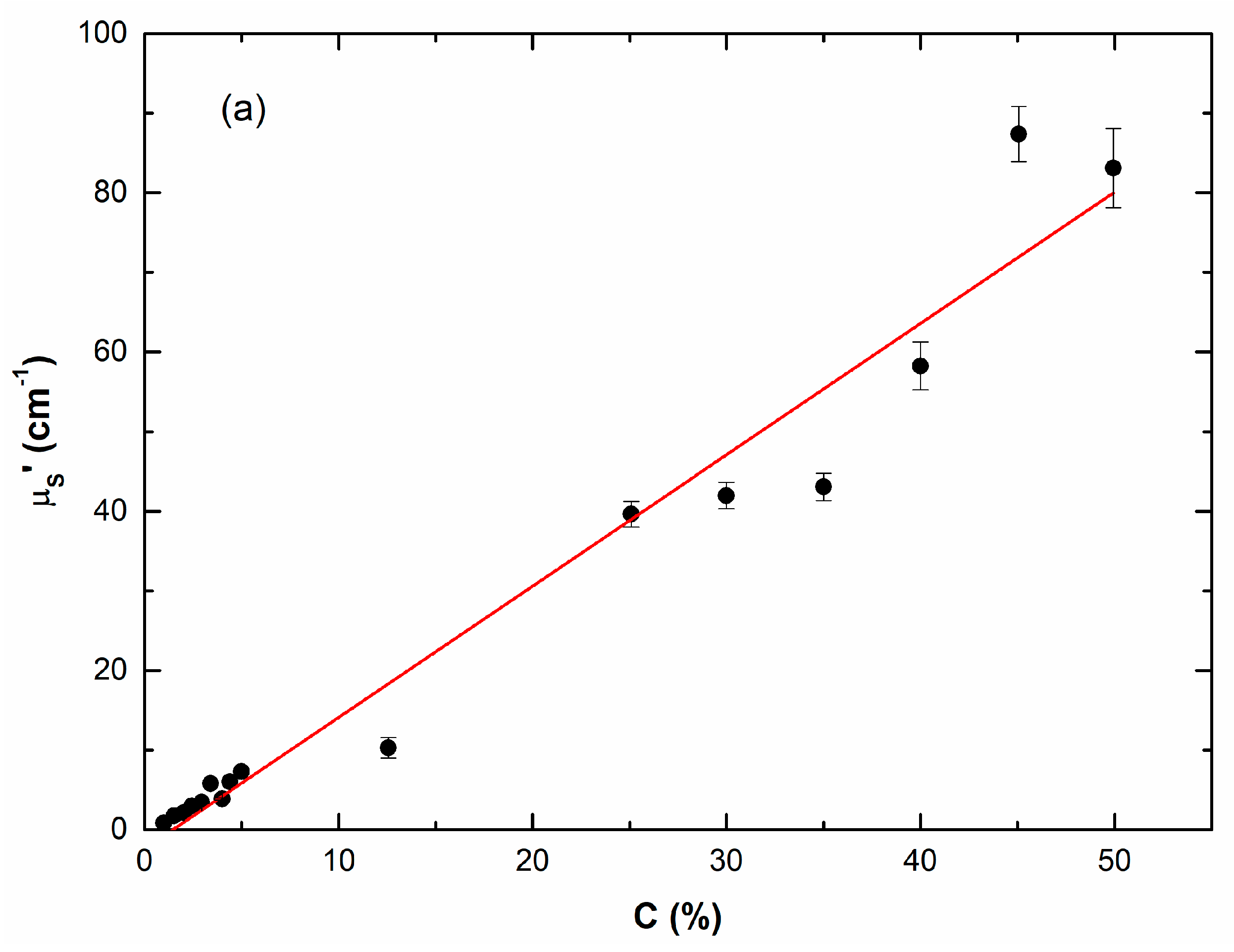
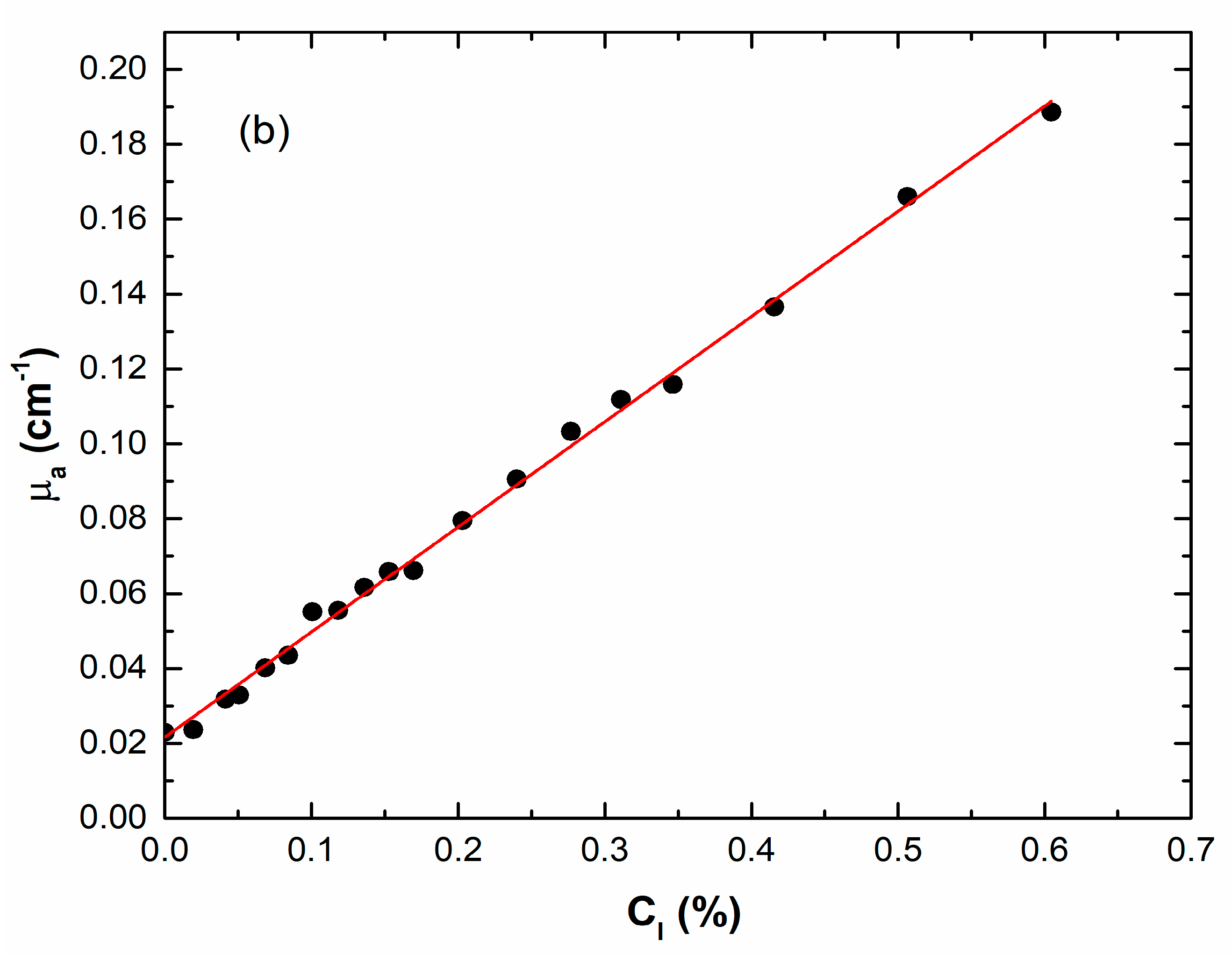
4.3.1. Homogeneous Slab Results
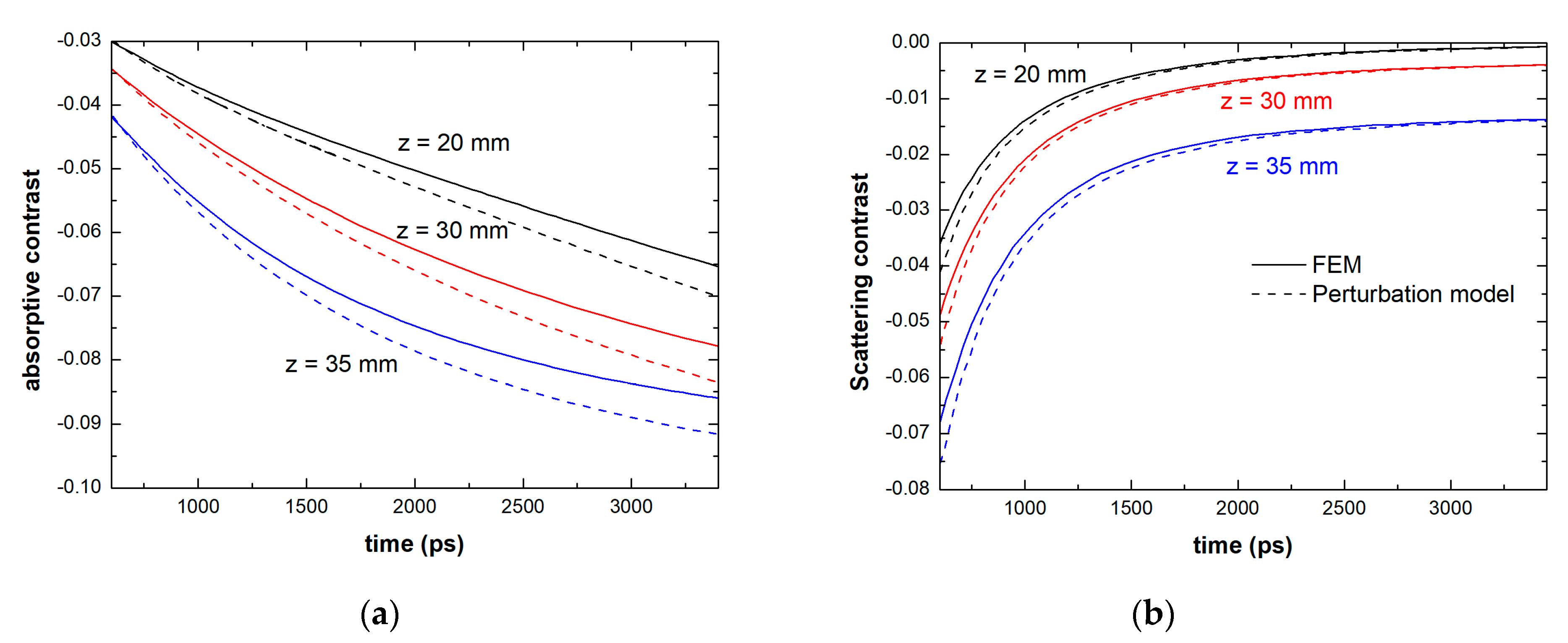
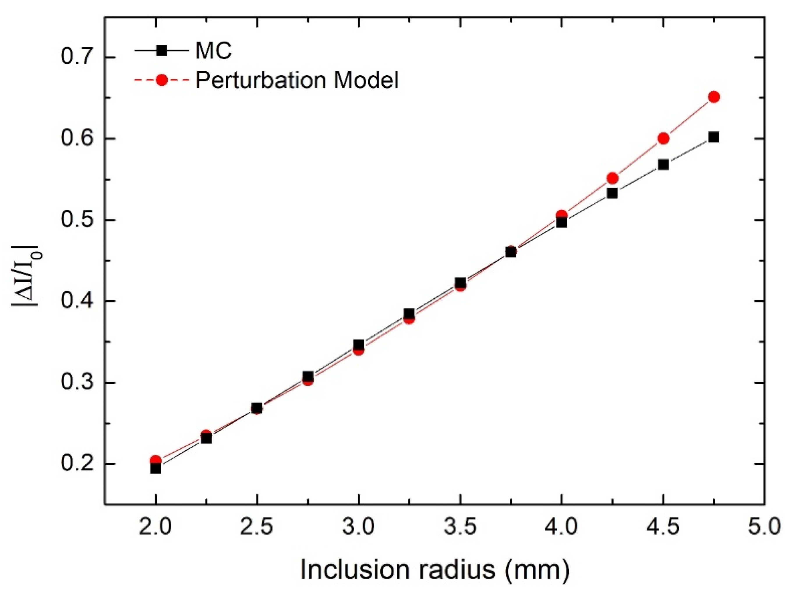
4.3.2. Absorptive Inclusion Results
5. Conclusions
Author Contributions
Funding
Conflicts of Interest
References
- Ruiz, C.C.; Molina-Bolıvar, J.A.; Aguiar, J. Thermodynamic and Structural Studies of Triton X-100 Micelles in Ethylene Glycol-Water Mixed Solvents. Langmuir 2001, 17, 6831–6840. [Google Scholar] [CrossRef]
- Berne, B.J.; Pecora, R. Dynamic Light Scattering; Wiley-Interscience: New York, NY, USA, 1976. [Google Scholar]
- Kerker, M. The Scattering of Light, and Other Electromagnetic Radiations; Academic Press: New York, NY, USA, 1969. [Google Scholar]
- Pine, D.J.; Weitz, D.A.; Chaikin, P.M.; Herbolzheimer, E. Diffusing-wave spectroscopy. Phys. Rev. Lett. 1988, 60, 1134–1137. [Google Scholar] [CrossRef] [PubMed]
- Corredig, M.; Alexander, M. Food emulsions studied by DWS: Recent advances. Trends Food Sci. Technol. 2008, 19, 67–75. [Google Scholar] [CrossRef]
- Kwan, T.O.C.; Reis, R.; Siligardi, G.; Hussain, R.; Cheruvara, H.; Moraes, I. Selection of Biophysical Methods for Characterisation of Membrane Proteins. Int. J. Mol. Sci. 2019, 20, 2605. [Google Scholar] [CrossRef] [PubMed]
- Badruddoza, A.Z.M.; MacWilliams, S.V.; Sebbenb, D.A.; Krasowska, M.; Beattie, D.; Durian, D.J.; Ferri, J.K. Diffusing wave spectroscopy (DWS) methods applied to double emulsions. Curr. Opin. Colloid Interface Sci. 2018, 37, 74–87. [Google Scholar] [CrossRef]
- Delfino, I.; Piccolo, C.; Lepore, M. Experimental study of short- and long-time diffusion regimes of spherical particles in carboxymethylcellulose solutions. Eur. Pol. J. 2005, 41, 1772–1780. [Google Scholar] [CrossRef]
- Martins, S.; Martins, I.C.; Santos, N.C. Methods for Lipid Droplet Biophysical Characterization in Flaviviridae Infections. Front. Microbiol. 2018, 9, 1951. [Google Scholar] [CrossRef]
- Jain, K.; Thareja, S. In vitro and in vivo characterization of pharmaceutical nanocarriers used for drug delivery. Artif. Cells Nanomed. Biotechnol. 2019, 47, 524–539. [Google Scholar] [CrossRef]
- Niu, F.; Ahmada, M.; Fana, J.; Ritzoulis, C.; Chen, J.; Luo, Z.; Pana, W. The application of diffusing wave spectroscopy (DWS) in soft foods. Food Hydrocoll. 2019, 96, 671–680. [Google Scholar] [CrossRef]
- Xu, J.; Liu, S.X.; Boddu, V.M. Micro-rheological and micro-heterogeneity properties of soluble glutinous rice starch (SGRS) solutions studied by diffusing wave spectroscopy (DWS). J. Food Meas. Charact. 2019, 13, 2822–2827. [Google Scholar] [CrossRef]
- Carvalho, P.M.; Felício, M.R.; Santos, N.C.; Gonçalves, S.; Domingues, M.M. Application of Light Scattering Techniques to Nanoparticle Characterization and Development. Front. Chem. 2018, 6, 237. [Google Scholar] [CrossRef] [PubMed]
- Maguire, C.M.; Rösslein, M.; Wickc, P.; Prina-Mello, A. Characterisation of particles in solution–a perspective on light scattering and comparative technologies. Sci. Technol. Adv. Mater. 2018, 19, 732–745. [Google Scholar] [CrossRef] [PubMed]
- Sharma, S.; Jaiswal, S.; Duffy, B.; Jaiswal, A.K. Nanostructured Materials for Food Applications: Spectroscopy, Microscopy and Physical Properties. Bioengineering 2019, 6, 26. [Google Scholar] [CrossRef] [PubMed]
- Minton, A.P. Recent applications of light scattering measurement in the biological and biopharmaceutical sciences. Anal. Biochem. 2016, 501, 4–22. [Google Scholar] [CrossRef]
- Zhou, W.; Kholiqov, O.; Chong, S.P.; Srinivasan, V.J. Highly parallel, interferometric diffusing wave spectroscopy for monitoring cerebral blood flow dynamics. Optica 2018, 5, 518–527. [Google Scholar] [CrossRef] [PubMed]
- Yamada, Y.; Suzuki, H.; Yamashita, Y. Time-Domain Near-Infrared Spectroscopy and Imaging: A Review. Appl. Sci. 2019, 9, 1127. [Google Scholar] [CrossRef]
- Delfino, I.; Lepore, M.; Indovina, P.L. Experimental tests of different solutions to the diffusion equation for optical characterization of scattering media by time-resolved transmittance. Appl. Opt. 1999, 38, 4228–4236. [Google Scholar] [CrossRef]
- Esposito, R.; Brambilla, M.; Pifferi, A.; Spinelli, L.; De Nicola, S.; Lepore, M. Depth dependence of estimated optical properties of a scattering inclusion by time-resolved contrast function. Opt. Express 2008, 16, 17667–17681. [Google Scholar] [CrossRef]
- Kholiqov, O.; Zhou, W.; Zhang, T.; Le, V.N.D.; Srinivasan, V.J. Time-of-flight resolved light field fluctuations reveal deep human tissue physiology. Nat. Commun. 2020, 11, 391. [Google Scholar] [CrossRef]
- Nicolai, B.M.; Beullens, K.; Bobelyn, E.; Peirs, A.; Saeys, W.; Theron, K.I.; Lammertyn, J. Review Nondestructive measurement of fruit and vegetable quality by means of NIR spectroscopy: A review. Postharvest Biol. Technol. 2007, 46, 99–118. [Google Scholar] [CrossRef]
- Torricelli, A.; Spinelli, L.; Contini, D.; Vanoli, M.; Rizzolo, A.; Zerbini, P.E. Time-resolved reflectance spectroscopy for non-destructive assessment of food quality. Sens. Instrum. Food Qual. Saf. 2008, 2, 82–89. [Google Scholar] [CrossRef]
- Torricelli, A.; Contini, D.; Mora, A.D.; Martinenghi, E.; Tamborini, D.; Villa, F.; Tosi, A.; Spinelli, L. Recent advances in time-resolved nir spectroscopy for nondestructive assessment of fruit quality. Chem. Eng. Trans. 2015, 44, 43–48. [Google Scholar]
- Rizzolo, A.; Vanoli, M. Time-Resolved Technique for Measuring Optical Properties and Quality of Food. In Light Scattering Technology for Food Property, Quality and Safety Assessment; Lu, R., Ed.; CRC Press Taylor & Francis Group: Oxfordshire, UK, 2016; pp. 187–224. [Google Scholar] [CrossRef]
- Milej, D.; Kruczkowski, M.; Kacprzak, M.; Sawosz, P.; Maniewski, R.; Liebert, A. Estimation of light detection efficiency for different light guides used in time-resolved near-infrared spectroscopy. Biocybern. Biomed. Eng. 2015, 35, 227–231. [Google Scholar] [CrossRef]
- Park, J.H.; Park, J.; Lee, K.R.; Park, Y.K. Disordered optics: Exploiting multiple light scattering and wavefront shaping for nonconventional optical elements. Adv. Mater. 2019, 32, 1903457. [Google Scholar] [CrossRef]
- Bohren, C.F.; Huffman, D.R. Absorption and Scattering of Light by Small Particles; John Wiley & Sons: New York, NY, USA, 1983. [Google Scholar]
- Ishimaru, A. Wave Propagation and Scattering in Random Media; Academic Press: New York, NY, USA, 1978. [Google Scholar]
- Pierrat, R.; Greffet, J.-J.; Carminati, R. Photon diffusion coefficient in scattering and absorbing media. J. Opt. Soc. Am. A 2006, 23, 1106–1110. [Google Scholar] [CrossRef]
- Delfino, I.; Esposito, R.; Piccirillo, B.; Lepore, M. Static and dynamic light scattering properties of Intralipid aqueous suspensions for tissue phantoms preparation and calibration. Proc. SPIE 2008, 6870, 68700P. [Google Scholar] [CrossRef]
- Cletus, B.; Künnemeyer, R.; Martinsen, P.; McGlone, V.A. Temperature-dependent optical properties of Intralipid measured with frequency-domain photon-migration spectroscopy. J. Biomed. Opt. 2010, 15, 017003. [Google Scholar] [CrossRef][Green Version]
- Ninni, P.D.; Martelli, F.; Zaccanti, G. Intralipid: Towards a diffusive reference standard for optical tissue phantoms. Phys. Med. Biol. 2011, 56, N21–N28. [Google Scholar] [CrossRef]
- Rowe, P.I.; Künnemeyer, R.; McGlone, R.; Talele, S.; Martinsen, P.; Oliver, R. Thermal stability of intralipid optical phantoms. Appl. Spectrosc. 2013, 67, 993–996. [Google Scholar] [CrossRef]
- Cipelletti, L.; Trappe, V.; Pine, D.J. Scattering Techniques. In Fluids, Colloids and Soft Materials: An Introduction to Soft Matter Physics; Nieves, A.F., Puertas, A.F., Eds.; John Wiley & Sons, Inc.: New York, NY, USA, 2016. [Google Scholar]
- Murphy, R.M. Murphy Static and dynamic light scattering of biological macromolecules: What can we learn? Opin. Biotechnol. 1997, 8, 25–30. [Google Scholar] [CrossRef]
- Sassaroli, A.; Martelli, F.; Fantini, S. Perturbation theory for the diffusion equation by use of the moments of the generalized temporal point-spread function. III. Frequency-domain and time-domain results. J. Opt. Soc. Am. A 2010, 27, 1723–1742. [Google Scholar] [CrossRef] [PubMed]
- Contini, D.; Martelli, F.; Zaccanti, G. Photon migration through a turbid slab described by a model based on diffusion approximation. I. Theory. Appl. Opt. 1997, 36, 4587–4599. [Google Scholar] [CrossRef] [PubMed]
- Esposito, R.; Martelli, F.; De Nicola, S. Closed-form solution of the steady-state photon diffusion equation in the presence of absorbing inclusions. Opt. Lett. 2014, 39, 826–829. [Google Scholar] [CrossRef] [PubMed][Green Version]
- Van Staveren, H.J.; Moes, C.J.; van Marie, J.; Prahl, S.A.; van Gemert, M.J.C. Light scattering in Intralipid-10% in the wavelength range of 400–1100nm. Appl. Opt. 1991, 30, 4507–4514. [Google Scholar] [CrossRef] [PubMed]
- Cubeddu, R.; Pifferi, A.; Taroni, P.; Torricelli, A.; Valentini, G. A solid tissue phantom for photon migration studies. Phys. Med. Biol. 1997, 42, 1971–1979. [Google Scholar] [CrossRef] [PubMed]
- Stetefeld, J.; McKenna, S.A.; Patel, T.R. Dynamic light scattering: A practical guide and applications in biomedical sciences. Biophys. Rev. 2016, 8, 409–427. [Google Scholar] [CrossRef] [PubMed]
- Chernomordik, V.; Gandjbakhche, A.; Lepore, M.; Esposito, R.; Delfino, I. Depth dependence of the analytical expression for the width of the point spread function (spatial resolution) in time resolved transillumination. J. Biomed. Opt. 2001, 6, 441–445. [Google Scholar] [CrossRef][Green Version]
- Delfino, M.I.; Lepore, M.; Indovina, P.L. Experimental evaluation of absorption coefficient in scattering media using different solutions to the diffusion equation. Phys. Med. 2002, XVIII, 124–136. [Google Scholar]
- Wiersma, D.S.; Muzzi, A.; Colocci, M.; Righini, R. Time-resolved experiments on light diffusion in anisotropic random media. Phys. Rev. E 2000, 62, 6681–6687. [Google Scholar] [CrossRef]
- Feder, I.; Duadi, H.; Fixler, D. Experimental system for measuring the full scattering profile of circular phantoms. Biomed. Opt. Express 2015, 6, 2877–2886. [Google Scholar] [CrossRef]
- Spinelli, L.; Martelli, F.; Farina, A.; Pifferi, A.; Torricelli, A.; Cubeddu, R.; Zaccanti, G. Calibration of scattering and absorption properties of a liquid diffusive medium at NIR wavelengths. Time-resolved method. Opt. Express 2007, 15, 6589–6604. [Google Scholar] [CrossRef] [PubMed]


© 2020 by the authors. Licensee MDPI, Basel, Switzerland. This article is an open access article distributed under the terms and conditions of the Creative Commons Attribution (CC BY) license (http://creativecommons.org/licenses/by/4.0/).
Share and Cite
Delfino, I.; Lepore, M.; Esposito, R. Optical Characterization of Homogeneous and Heterogeneous Intralipid-Based Samples. Appl. Sci. 2020, 10, 6234. https://doi.org/10.3390/app10186234
Delfino I, Lepore M, Esposito R. Optical Characterization of Homogeneous and Heterogeneous Intralipid-Based Samples. Applied Sciences. 2020; 10(18):6234. https://doi.org/10.3390/app10186234
Chicago/Turabian StyleDelfino, Ines, Maria Lepore, and Rosario Esposito. 2020. "Optical Characterization of Homogeneous and Heterogeneous Intralipid-Based Samples" Applied Sciences 10, no. 18: 6234. https://doi.org/10.3390/app10186234
APA StyleDelfino, I., Lepore, M., & Esposito, R. (2020). Optical Characterization of Homogeneous and Heterogeneous Intralipid-Based Samples. Applied Sciences, 10(18), 6234. https://doi.org/10.3390/app10186234