Article

Assessment of Earthquake Destructive Power to Structures Based on Machine Learning Methods

1
Guangdong Provincial Key Laboratory of Durability for Marine Civil Engineering, Shenzhen University, Shenzhen 518060, China
2
Key Laboratory of Urban Security and Disaster Engineering of Ministry of Education, Beijing University of Technology, Beijing 100124, China
*
Author to whom correspondence should be addressed.
Appl. Sci. 2020, 10(18), 6210; https://doi.org/10.3390/app10186210
Submission received: 10 August 2020 / Revised: 29 August 2020 / Accepted: 3 September 2020 / Published: 7 September 2020
(This article belongs to the Special Issue Structural and Earthquake Engineering)

Abstract

:
This study presents a machine learning-based method for the destructive power assessment of earthquake to structures. First, the analysis procedure of the method is presented, and the backpropagation neural network (BPNN) and convolutional neural network (CNN) are used as the machine learning algorithms. Second, the optimized BPNN architecture is obtained by discussing the influence of a different number of hidden layers and nodes. Third, the CNN architecture is proposed based on several classical deep learning networks. To build the machine learning models, 50,570 time-history analysis results of a structural system subjected to different ground motions are used as training, validation, and test samples. The results of the BPNN indicate that the features extraction method based on the short-time Fourier transform (STFT) can well reflect the frequency-/time-domain characteristics of ground motions. The results of the CNN indicate that the CNN exhibits better accuracy (R2 = 0.8737) compared with that of the BPNN (R2 = 0.6784). Furthermore, the CNN model exhibits remarkable computational efficiency, the prediction of 1000 structures based on the CNN model takes 0.762 s, while 507.81 s are required for the conventional time-history analysis (THA)-based simulation. Feature visualization of different layers of the CNN reveals that the shallow to deep layers of the CNN can extract the high to low-frequency features of ground motions. The proposed method can assist in the fast prediction of engineering demand parameters of large-number structures, which facilitates the damage or loss assessments of regional structures for timely emergency response and disaster relief after earthquake.

1. Introduction

Destructive earthquake is a tremendous threat to the operation and security of civil infrastructures. For example, the Wenchuan earthquake in 2008 caused the collapse of a large number of buildings, resulting in more than 65,000 deaths [1]. Moreover, the Northridge earthquake in 1994 damaged California’s transportation infrastructures, which seriously jeopardizes the transportation system [2]. The rapid assessment of earthquake destructive power to structures can provide a scientific basis for decision-makers, to facilitate the post-earthquake rescue and relief work.
The earthquake destructive power to structures is influenced by the frequency-/time-domain characteristics of ground motions and the nonlinear seismic performance of structures. In previous studies, the seismic fragility analysis [3] and capacity spectrum method [4] have been frequently used to assess the earthquake’s destructive power to regional infrastructures [5,6]. With the advancement of high-performance computing technologies and the higher accuracy requirement for seismic damage assessment, the time-history analysis (THA)-based method is gradually applied to the seismic damage simulation of regional infrastructures [7,8,9,10,11]. The THA-based seismic damage simulation method can adequately consider the frequency-/time-domain characteristics of ground motions and the nonlinear seismic performance of structures, to reasonably reflect the destructive power of earthquake to structures. Furthermore, the THA-based seismic damage simulation method can be applied to different types of structural systems and reveal the whole process of failure mechanism of a structure [11,12]. Therefore, the THA-based seismic damage simulation is adopted as the benchmark method in this study.
To date, machine learning methods have been widely used in various fields, such as the recognition of visual objects, natural language, and music [13,14,15,16]. Moreover, there are also many applications of machine learning methods in earthquake engineering [17,18,19,20,21,22,23,24,25]. Xu et al. [17] used several machine learning methods to predict structural types based on regional building attribute data. Mangalathu et al. [18] suggested an artificial neural network-based multi-parameter fragility methodology that can generate bridge-specific fragility curves without grouping the bridge classes. Nguyen et al. [19] proposed a hybrid particle-swarm-optimization-based artificial neural network model to calculate horizontal displacement of columns subjected to an earthquake. Zhang et al. [20] proposed a physical-guided convolutional neural network, which can make full use of the physical model and only adopt a small training dataset to realize an accurate simulation of structural responses. Kiani et al. [21] proposed a structural fragility curve generation method based on multiple machine learning methods. Xiong et al. [22] proposed an automated building seismic damage assessment method using an uncrewed aerial vehicle (UAV) and a convolutional neural network (CNN), which can obtain the damage distribution of an area with an accuracy of 89.39%. Moreover, extensive research works have been reported on the machine learning-based seismic response simulation (Table 1). Mangalathu et al. [23,24] adopt various machine learning methods to predict the damage state of a structure. It is a classification problem, and the computational workload of the simulation is light. Nevertheless, in some cases, obtaining engineering demand parameters (EDPs) is more favorable for damage or loss assessment of a structure. In the study of Zhang et al. [25], long-short-term memory (LSTM) [26] network is used to predict the structural time-history response. The LSTM network requires a relatively large computational workload [27] and is not suitable for the response prediction of a large number of structures.
This study focuses on the fast prediction of EDP under seismic excitation. Considering that the backpropagation neural network (BPNN) [28] and CNN [13] models are capable of simulating complex nonlinear problems and exhibit good computational efficiency, these two models are used to predict the EDP of structures subjected to earthquake, to reflect the destructive power of earthquake to structures. Specifically, in Section 2, the analysis procedure of the method is introduced; in Section 3, the details of the adopted structural model and the ground motion records are presented; in Section 4, two feature extraction methods of ground motions are proposed, and the BPNN is used to assess the earthquake destructive power to structures; in Section 5, the CNN is adopted to extract the features of ground motions and predict the earthquake destructive power to structures. The proposed method aims to realize a rapid evaluation of earthquake destructive power to structures based on machine learning methods. It is expected to provide a useful reference for timely emergency response and disaster relief after the earthquake.

2. Analysis Procedure of the Proposed Method

Nonlinear THA of structures can well capture the frequency-/time-domain characteristics of ground motions and the elasto-plastic mechanical properties of structures—therefore, it is used to calculate the seismic responses of structures which forms the training set. The simulation framework proposed in this study mainly consists of two modules, which are sample preparation and machine learning method, as shown in Figure 1. The sample preparation module presents details of the structural system, ground motion records, and how each sample for model training is obtained. In the machine learning module, the BPNN and CNN are adopted as the specific machine learning methods, of which the model architecture and simulation results are given in Section 4 and Section 5, respectively. The detailed simulation procedures are as follows:
  • Establish the nonlinear finite element model of a structure, and perform nonlinear THA of the structure subjected for a large number of ground motion records. The structural response data (e.g., maximum displacement and acceleration), together with ground motion data, are collected as a training sample.
  • Process the training sample data according to the machine learning method adopted. For example, extract feature parameters from ground motion records or adjust the ground motion records to identical lengths.
  • Feed the machine learning model with the processed sample data and obtain the well-tuned machine learning model.
  • Apply the well-tuned machine learning model and assess the destructive power of a new ground motion record by predicting the EDP, such as the maximum displacement of a structure.
Considering that the damage assessment methods and damage limits of different structures are different [4,29,30], the maximum displacement of a structure is adopted as the EDP to evaluate the earthquake destructive power to structures in this study. For other EDPs, such as maximum acceleration and maximum inter-story drift ratio, the method proposed in this study can also be adopted by retraining the machine learning model with training samples, including the adopted EDP.

3. Sample Preparation

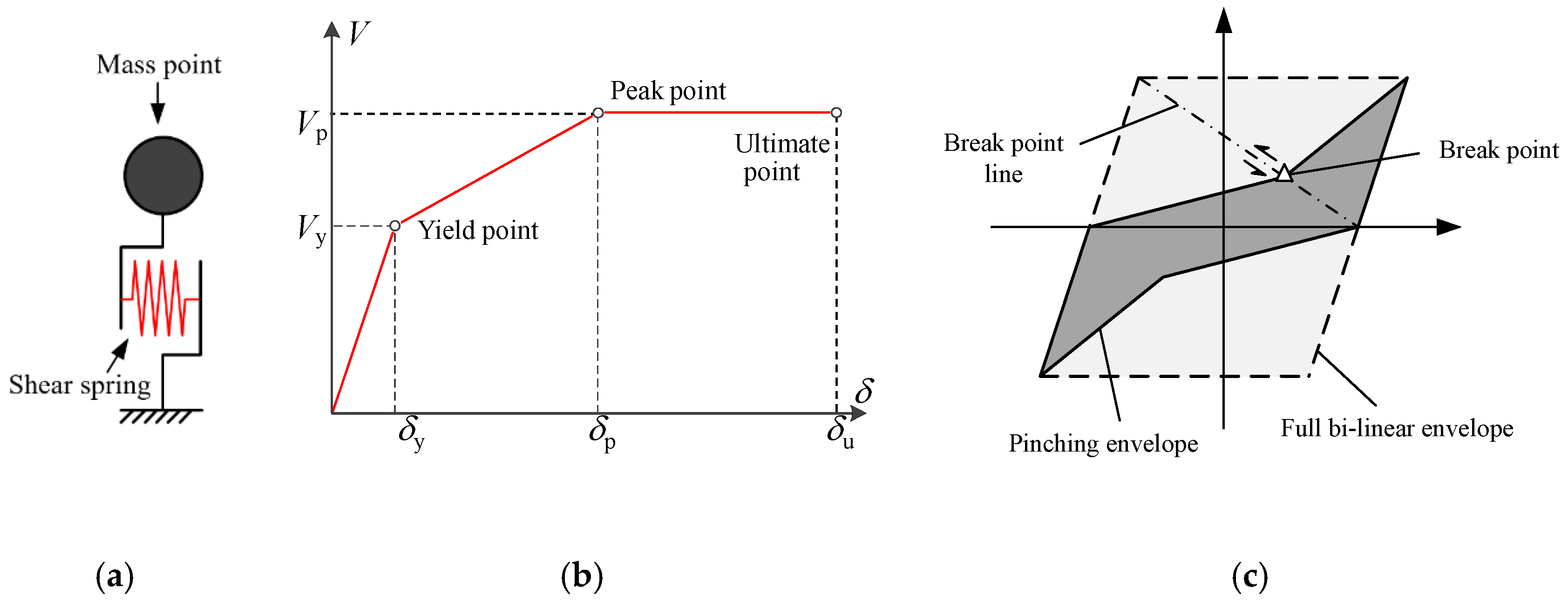
In this study, a relatively simple structural model named elasto-plastic single degree-of-freedom (SDOF) model is adopted, as shown in Figure 2a. The model can capture the elasto-plastic mechanical properties of multi-story buildings and simple girder bridges [31,32]. The elastic parameters of the SDOF model include the natural vibration period and the elastic damping ratio. A tri-linear backbone curve is adopted for the interstory performance of the SDOF model, as shown in Figure 2b [4]. The parameters of the backbone curve parameter include yield strength to weight ratio, peak to yield strength ratio, and the secondary stiffness ratio. The secondary stiffness ratio is defined by the ratio of post-yield stiffness to the elastic stiffness. A single-parameter hysteretic model is adopted for the SDOF system (Figure 2c). The hysteretic parameters reflect the ratio of the hysteretic area of the pinching model to that of the full bi-linear model (Figure 2c). The parameters of the elasto-plastic SDOF model adopted in this paper are shown in Table 2.
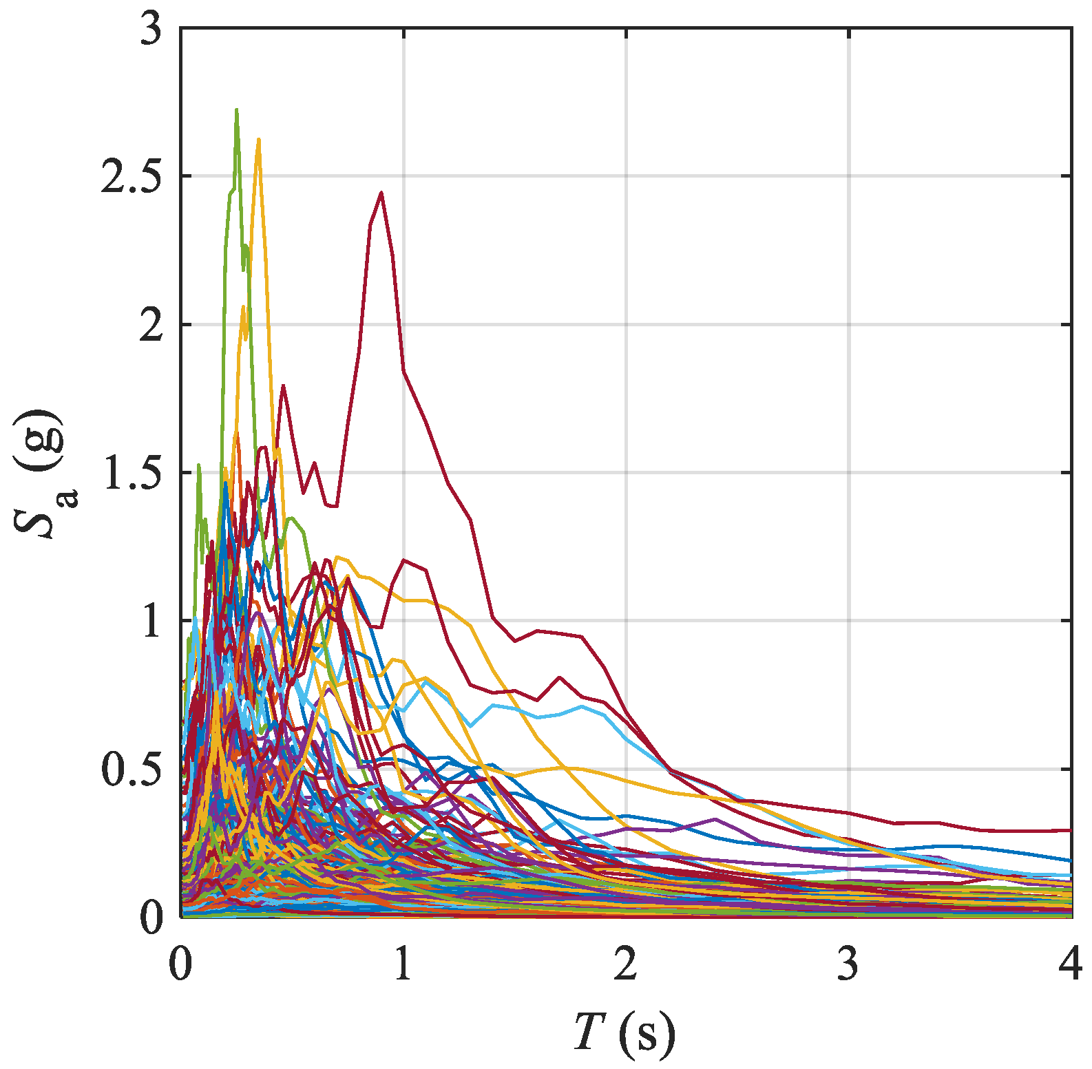
Considering that the characteristics of different ground motions vary significantly, to cover different types of ground motions as much as possible, 5057 ground motion records were collected from the pacific earthquake engineering research (PEER) center ground motion database [33]. The obtained ground motions were recorded from 1935 to 2003, of which earthquake magnitude ranges from 4.2 to 7.9. Most of the ground motions were recorded in the US and Japan. Some typical earthquakes are Chi-Chi, El Centro, Northridge, Landers, and Kobe earthquakes. The acceleration response spectra of some selected ground motions are shown in Figure 3. As evident in Figure 3, the randomness of different ground motions is significant. To expand the training data for better generalization of the machine learning model, the ground motion records are normalized and rescaled to ten different peak ground accelerations (PGA) (i.e., PGA = 1 − 10 m/s2), respectively. As a result, 50,570 ground motion acceleration sequences are obtained. Subsequently, THAs are performed to obtain the maximum response displacements of the SDOF model subjected to 50,570 ground motions. Finally, 50,570 ground motion acceleration sequences, together with the corresponding maximum response displacements, are taken as the dataset for model training.
The dataset is divided into a training set, a validation set, and a test set. According to the research of Ng [34], the test set should be large enough to give high confidence in the overall performance of the model. In this study, sample split experiments show that a test set size of 1000 can reasonably reflect the performance of the prediction model. Therefore, the original sample set is divided into 48,570, 1000, and 1000 samples for the training, validation, and test sets, respectively. It is worth noting that the original 50,570 sample set is generated using 5057 ground motion records in ten different PGAs. To makes sure that the ground motions in the test and validation sets are completely different from those in the training set, 4857, 100, and 100 ground motion records are randomly selected to generate the training, validation, and test sets, respectively.

4. Backpropagation Neural Network

The backpropagation neural network (BPNN) is a feed forward neural network, which has a backpropagation process. The backpropagation process repeatedly adjusts the weights of connections in the network, to minimize the difference between the actual output vector and the desired output vector [28].
The structure of the classic the BPNN usually consists of three layers, namely, the input layer, the hidden layer, and the output layer. The log-sigmoid function and the tan-sigmoid function are usually used as activation functions [18,35,36]. The BPNN has been widely used for its advantages of simple structure, stable performance, and easy to implement.

4.1. Feature Extractions

Ground motion records contain a large number of acceleration time-history data, which is well beyond the size of input suitable for the BPNN. Therefore, it is necessary to use appropriate methods to extract the features of ground motion data. The extracted features should contain enough information to reflect the destructive power of ground motion to structures. The size of the extracted feature should also be suitable for the implementation of the BPNN.
In the literature, the acceleration response spectrum of ground motion is usually used to characterize the destructive power of ground motion to structures [23]. The calculation of the response spectrum requires a large number of time-history analyses for SDOF systems with different natural vibration periods, which is computationally intensive. In a real post-earthquake scenario, many ground motion sequences will be recorded, and the calculation of the response spectra of many ground motion records is time-consuming. Compared with response spectrum analysis, the fast Fourier transform (FFT) algorithm is efficient and can extract the frequency-domain features of complex signals, which is widely used in various fields [37,38,39,40,41,42].
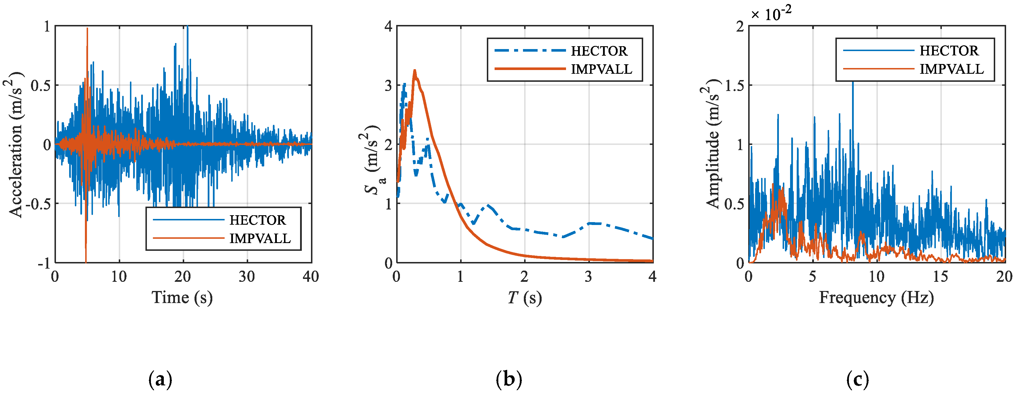
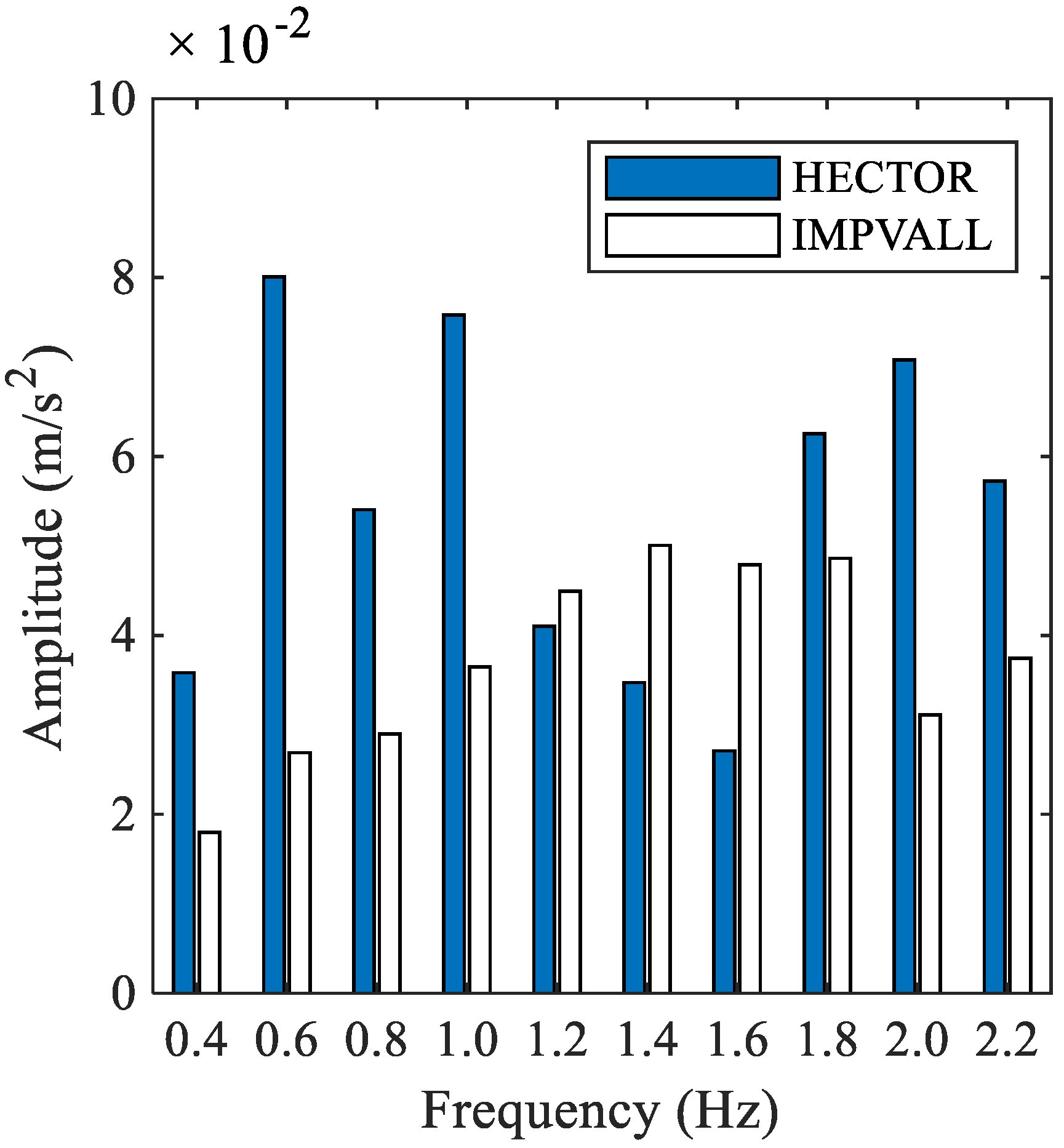
The feature extraction of two ground motions named HECTOR-0515A360 (hereinafter referred to as HECTOR) and IMPVALL-A-E06140 (hereinafter referred to as IMPVALL) (Figure 4a) [33] are discussed. Both ground motion records are normalized to 1 m/s2 for comparison. HECTOR’s vibration is strong in the whole 40 s range, while IMPVALL’s vibration mainly concentrates in the range of 3–7 s. By comparing the response spectra of the two ground motions (Figure 4b), it is found that the spectral acceleration of IMPVALL in the range of 0.3–1 s is greater than that of HECTOR. Considering that the natural vibration periods of multi-story buildings are usually within 0.3–1 s [43], the IMPVALL ground motion exhibits greater destructive power to these structures than the HECTOR ground motion. Nevertheless, the FFT spectrum (Figure 4c) indicates that the amplitude of IMPVALL is less than that of HECTOR in almost the entire frequency range. The difference between the response spectrum and FFT spectrum is that the seismic energy of the IMPVALL ground motion is released in a relatively short time. Therefore, the IMPVALL ground motion is very destructive to structures, even if its relatively low FFT spectrum compared to that of the HECTOR ground motion.
Previous studies have shown that the short-time Fourier transform (STFT) has a good performance in time-frequency domain analysis [44]. Therefore, this study proposes a ground motion feature extraction method based on the STFT algorithm. In consideration of the duration difference of ground motion records, all ground motions are truncated to the duration of 20 s. The specific process includes the following four steps:
  • Ground motion data truncation. Find the time point of the peak acceleration in a ground motion record, and truncate a 20 s signal with 10 s in both forward and backward. When the signals are less than 10 s in the front or back of the peak acceleration time point, the 20 s signal range should be shifted backward or forward to ensure that the peak acceleration is close to the center of the truncated signal.
  • STFT analysis. Considering that the selection of window size will affect the resolution of the STFT spectrum, the rectangular window length of 5 s and step length of 5 s are selected for the STFT analysis. Therefore, four frequency spectra of the 20 s truncated signal will be obtained.
  • Feature extraction. In this study, the natural vibration period of the adopted SDOF system is 0.5 s (Table 2). Considering that the period of the structure will be prolonged after entering the plastic state, the frequency range of interest is selected as 0.3–2.3 Hz. The interested frequency range of an STFT spectrum is divided into 10 frequency bands, and the corresponding spectral value of each frequency band is adopted as a feature value. Therefore, the feature extraction of four 5 s-windows yields 40 STFT spectral feature values.
  • Dimension setting of features. Considering that the number of feature values will affect the learning effect of the BPNN, two different dimensions of the feature are discussed in this study. One is to directly take the 40 STFT spectral values obtained in step (3). The other is to compute the maximum value of feature values in the same frequency range of four windows, which yields 10 feature values.
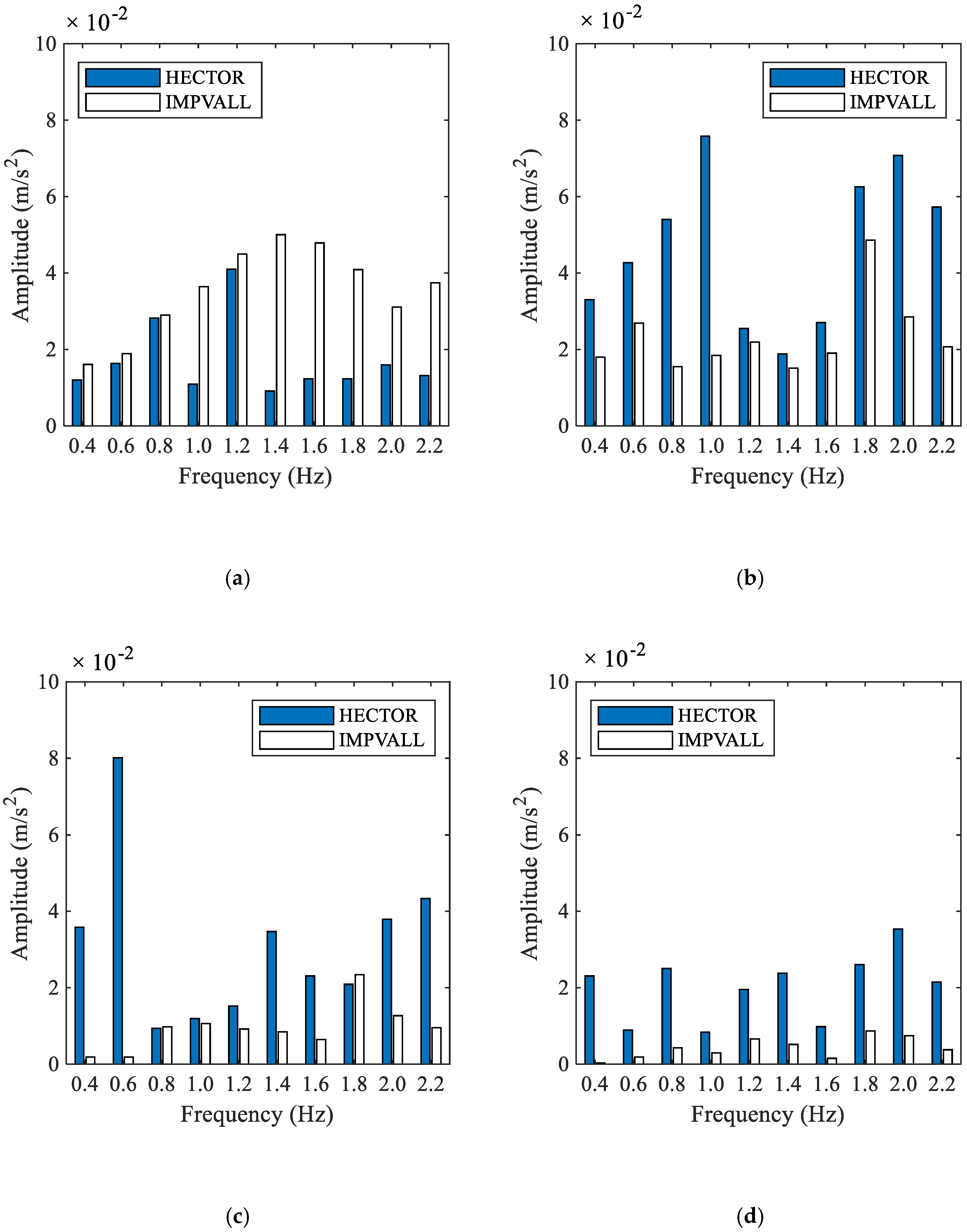
Based on the above methods, the ground motion features of HECTOR and IMPVALL are extracted, as shown in Figure 5 and Figure 6.
Figure 5a shows that the amplitude of IMPVALL in the range of 1.2–2.2 Hz is much higher than that of HECTOR. This result is consistent with the response spectrum results in Figure 4, and well reflects the destructive power of IMPVALL to structures in this frequency range. Figure 5b–d shows that the amplitude of IMPVALL is significantly lower than that of HECTOR. This is because the ground motion acceleration of IMPVALL is significantly lower than that of HECTOR in the time range of 7–20 s. From the above, the proposed feature extraction method based on STFT analysis can well reflect the frequency-/time-domain characteristics of ground motion sequences.
The 40 feature values of ground motion are further condensed by computing the maximum amplitude value of feature values in the same frequency band from four STFT spectra, which yields 10 feature values. As shown in Figure 6, the 10 feature values can still reflect the great destructive power of the IMPVALL ground motion to structures in the frequency range of 1.2–1.6 Hz. Therefore, the following section will discuss the training results using 40 and 10 feature values, respectively.

4.2. BPNN Architecture

The network structure, together with the input dimension, can greatly influence the prediction accuracy of a BPNN model [45,46]. Therefore, the influences of the number of hidden layers and nodes, as well as the dimension of features, are discussed to obtain the optimal BPNN architecture.
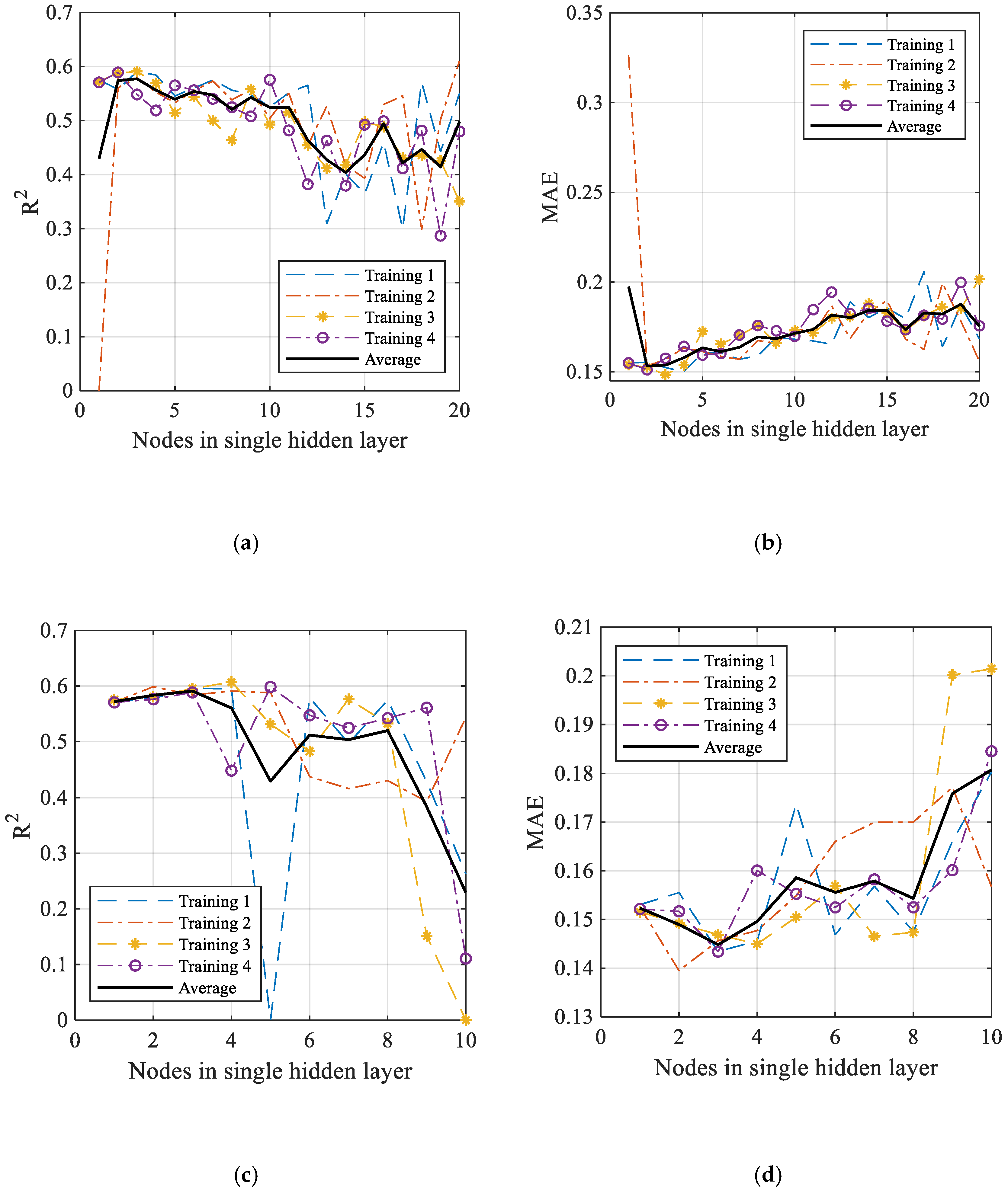
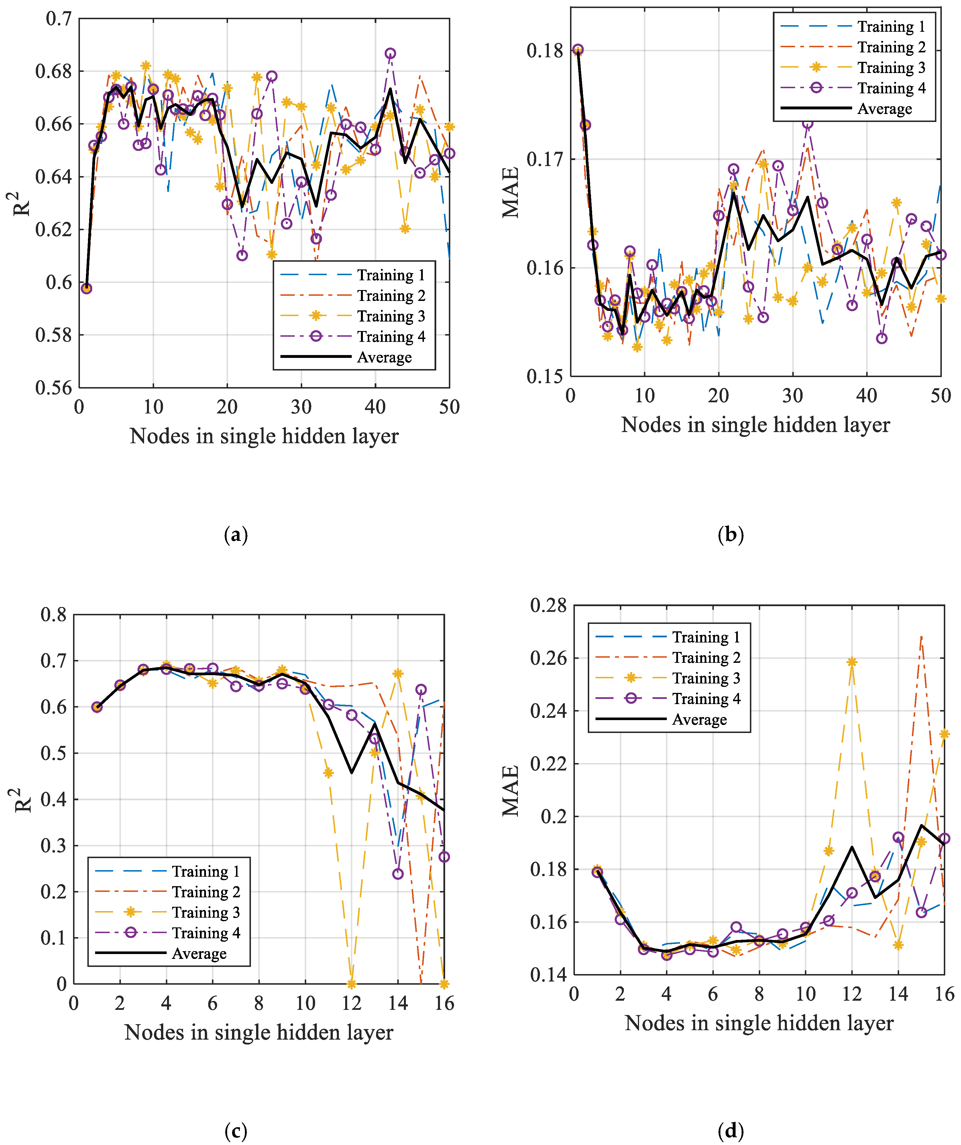
The R2 and mean absolute error (MAE) are used as evaluation indexes to select the optimal BPNN structure. The random initial weights are used for training, therefore, the results of each training are different. In this section, each BPNN structure was trained four times, respectively, the results are shown in Figure 7 and Figure 8.
For the cases with 40 feature values as input (Figure 7), with the increase of the number of nodes in the hidden layers, the prediction accuracy increases and then decreases. When the number of nodes reaching a certain number, the increase of nodes in the hidden layer can no longer improve the BPNN model.
The BPNN with a single hidden layer achieves the best prediction accuracy when the number of nodes is 3, of which the average R2 equals 0.5771, and the average MAE equals 0.1537. The BPNN with two hidden layers has the best prediction effect when the number of nodes in each layer is 3, with the average R2 equals 0.5910, and the average MAE equals 0.1448.
For the cases with 10 feature values as input, the result in Figure 8 indicates that with the increase of the number of nodes in the hidden layer, the accuracy of the model increases and then decreases. Moreover, if the number of nodes in the hidden layers further increases, the R2, and MAE indexes become unstable.
The BPNN with a single hidden layer achieves the best prediction accuracy when the number of nodes is 7, of which the average R2 equals 0.6740, and the average MAE equals 0.1539. The BPNN with two hidden layers has the best prediction effect when the number of nodes in each layer is 4, with the average R2 equals 0.6848, and the average MAE equals 0.1488.

4.3. Results of the BPNN

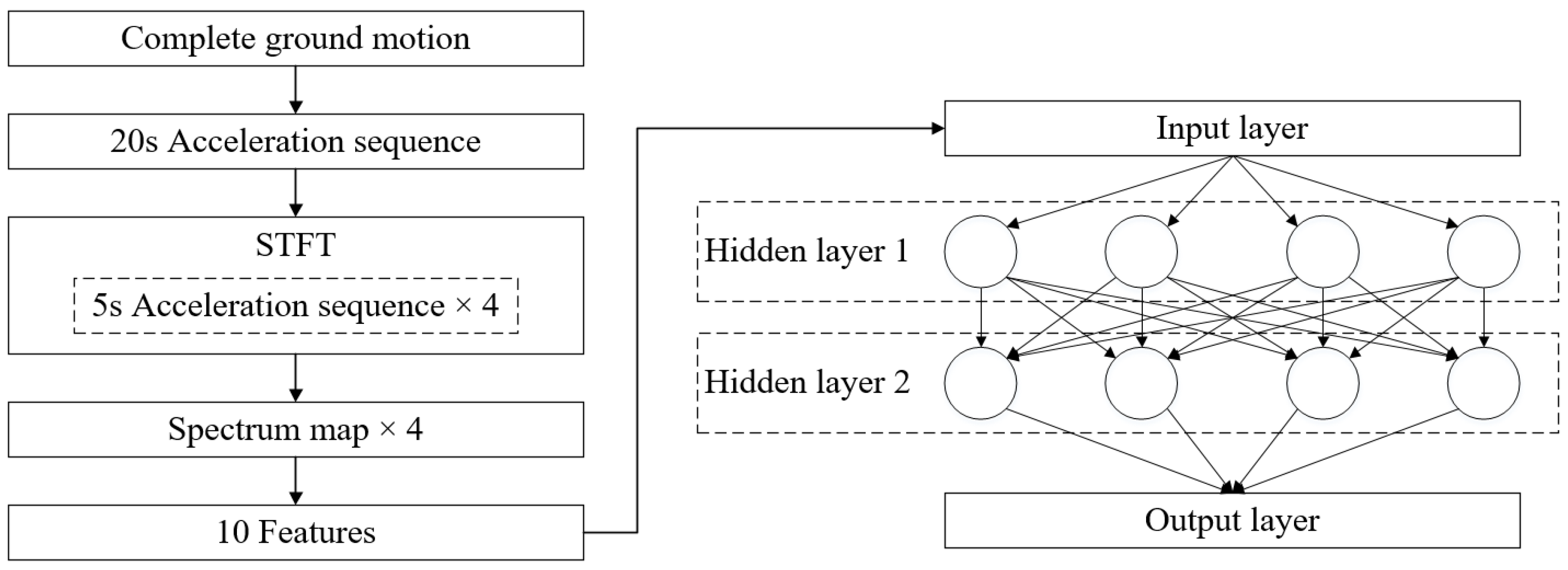
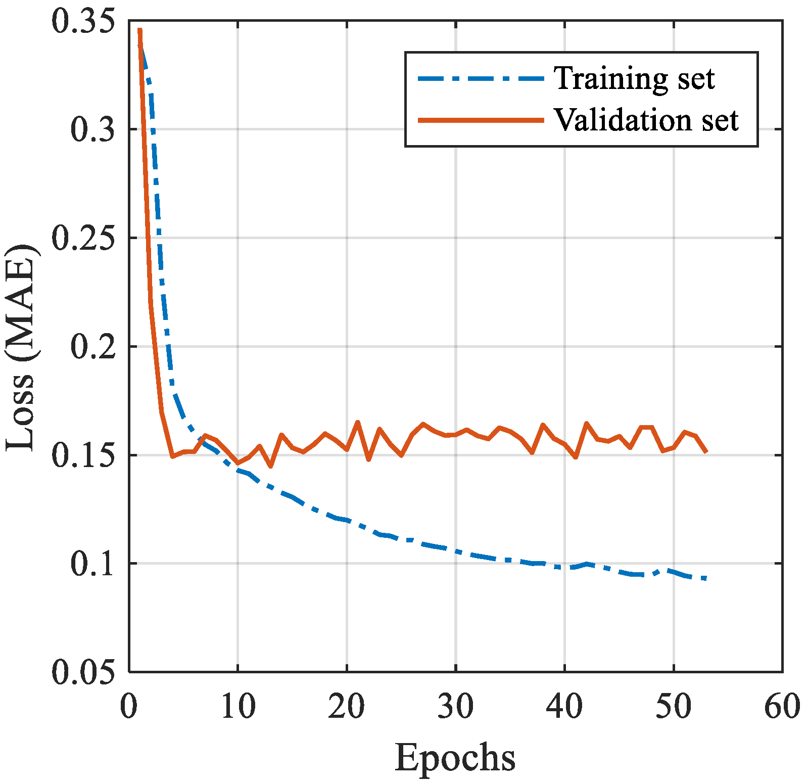
According to the discussion in Section 4.2, the 10-dimensional features are selected as the input. Moreover, the BPNN structure with two hidden layers and four nodes in each layer is selected. The schematic diagram of the feature extraction and network structure is illustrated in Figure 9. In the hidden layer of the BPNN, the nodes adopted the ReLU function as the activation function and Bayesian regularization algorithm as the training algorithm [47,48]. The learning algorithm is gradient descent with momentum [49], the loss function is MAE, the learning rate is 0.01, and the maximum training epochs is set to 500. The program adopts the EarlyStopping function [50], which can stop the training and output of the previous optimal model if the loss of validation cannot be improved in 40 epochs. The loss history of training and validation are shown in Figure 10.
The results show that in the early stage of training, the loss of training decreases with the increase of epoch. The loss of validation reaches the minimum (MAE = 0.1475) when the epoch is 13, and the program stopped training at the end of the 53rd epoch.
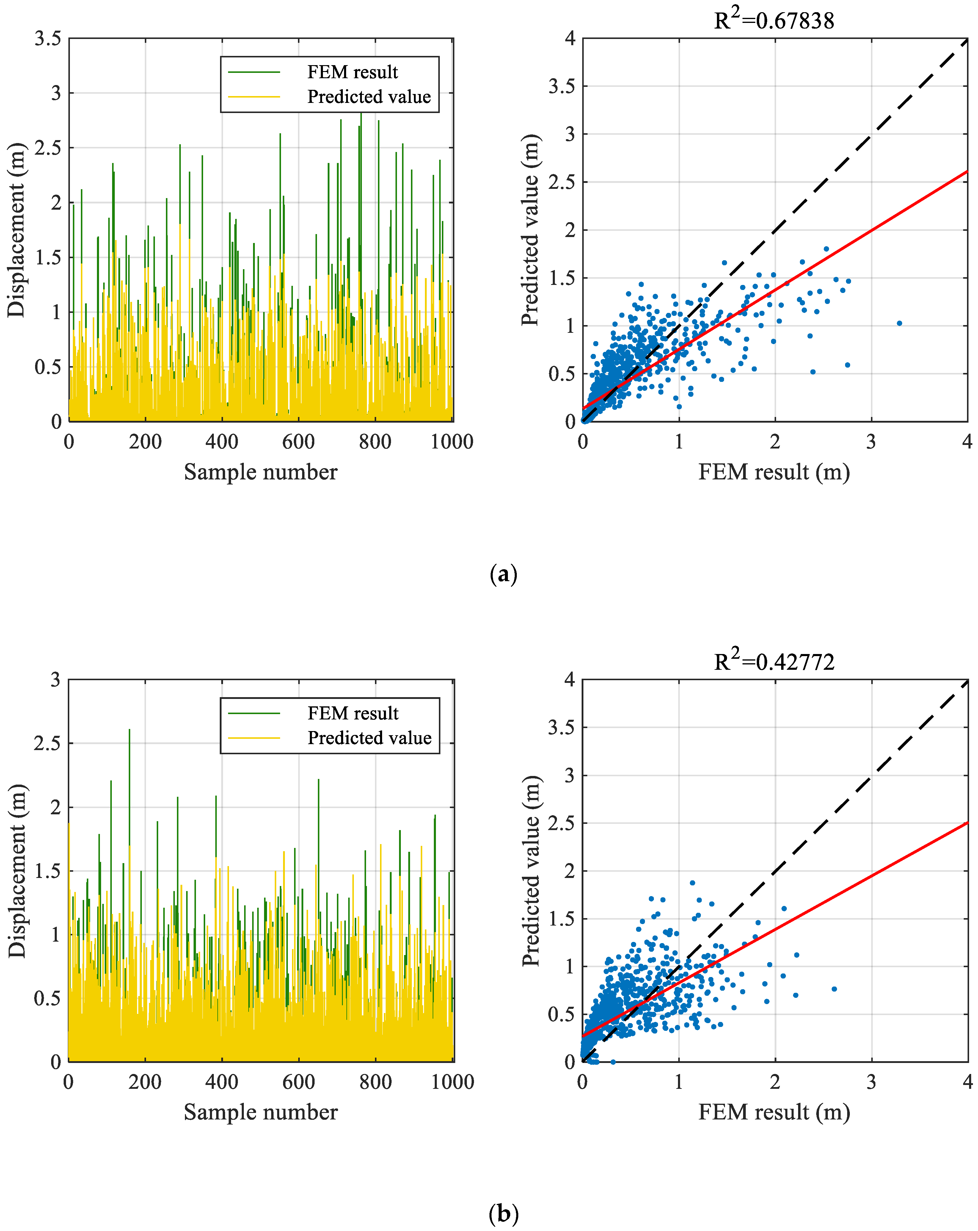
Finally, the test set is input into the optimal model, and the prediction results are shown in Figure 11. The statistical indexes of prediction errors are shown in Table 3. Evidently, the prediction results of the BPNN based on the STFT features are significantly better than those based on the FFT features. Nevertheless, both prediction results are poor. This is because the BPNN model is not capable of capturing the strong nonlinearity of the studied scenario. Therefore, a model based on the convolutional neural network is discussed in the subsequent section.

5. Convolutional Neural Network

Convolutional neural network (CNN) is also a feed forward neural network, which has excellent performance in image recognition [13] and the evaluation of one-dimensional sequences (such as sound signals) [51,52]. Therefore, the CNN is well suited for the feature extraction and evaluation of ground motion records.
The feature extraction process of the CNN is not designed by human engineers, but learned from data in the training process [14]. Therefore, features of ground motions can be learned in the convolutional layers, and manual feature extraction of ground motion data is not required.

5.1. CNN Architecture

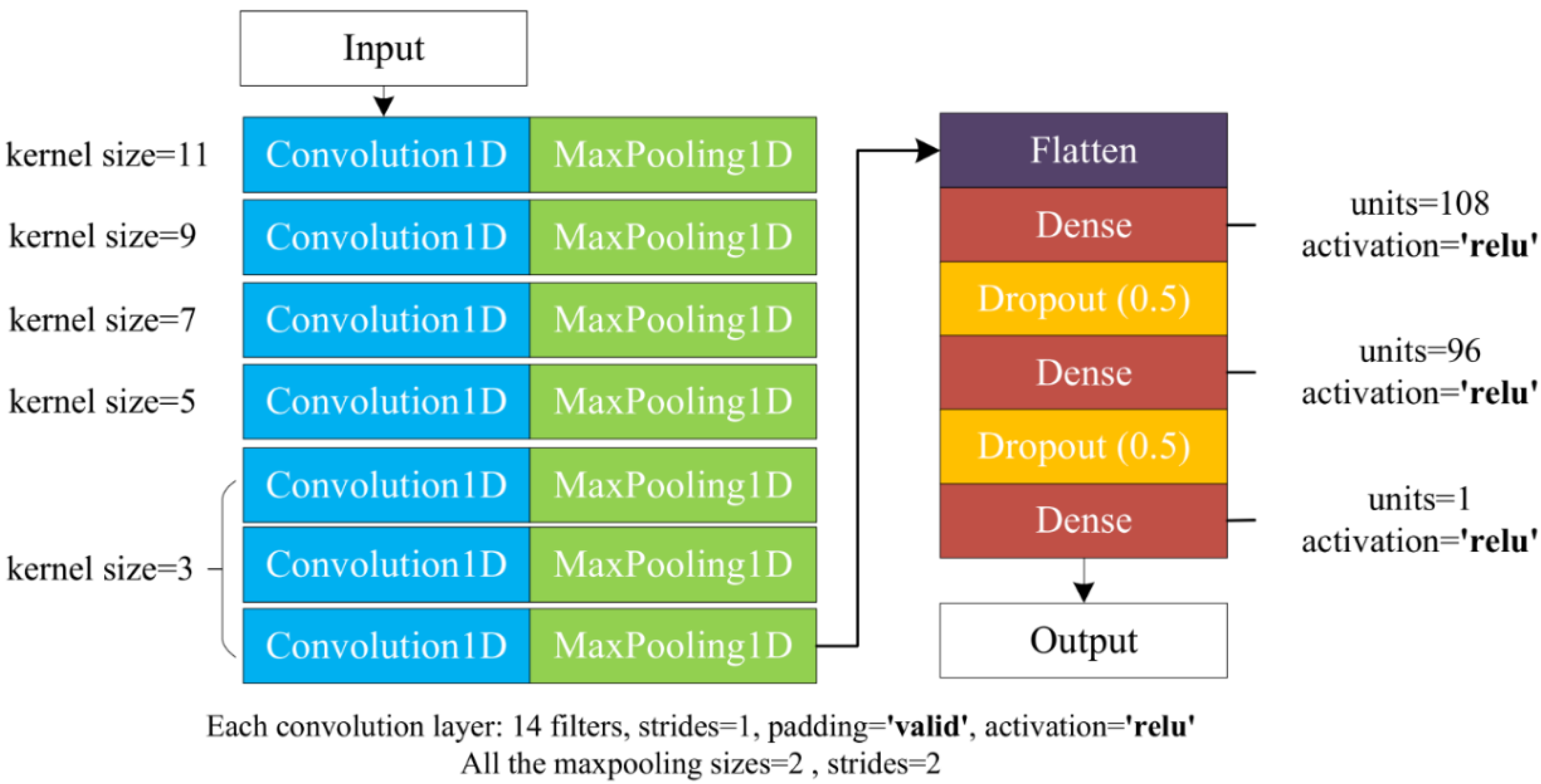
The architecture of some classical the CNN model, such as LeNet-5 [53], AlexNet [13], and Visual Geometry Group (VGG) [54] models are adopted as references to build the CNN architecture for ground motion evaluation. The CNN structure used in this study is illustrated in Figure 12.
All ground motion records are down sampled to 50 Hz and processed to 20 s signal sequences according to the method presented in Section 4.1. Therefore, 1000 data points of each ground motion are taken as the input for the proposed CNN model. The maximum response displacement of the structure under the action of ground motion is taken as the output. Adam algorithm was adopted as the optimization algorithm [55]. The loss function of MAE is adopted, the learning rate is set to 0.05, the maximum training epoch is set to 200, and the batch size is set to 4000.

5.2. Results of CNN

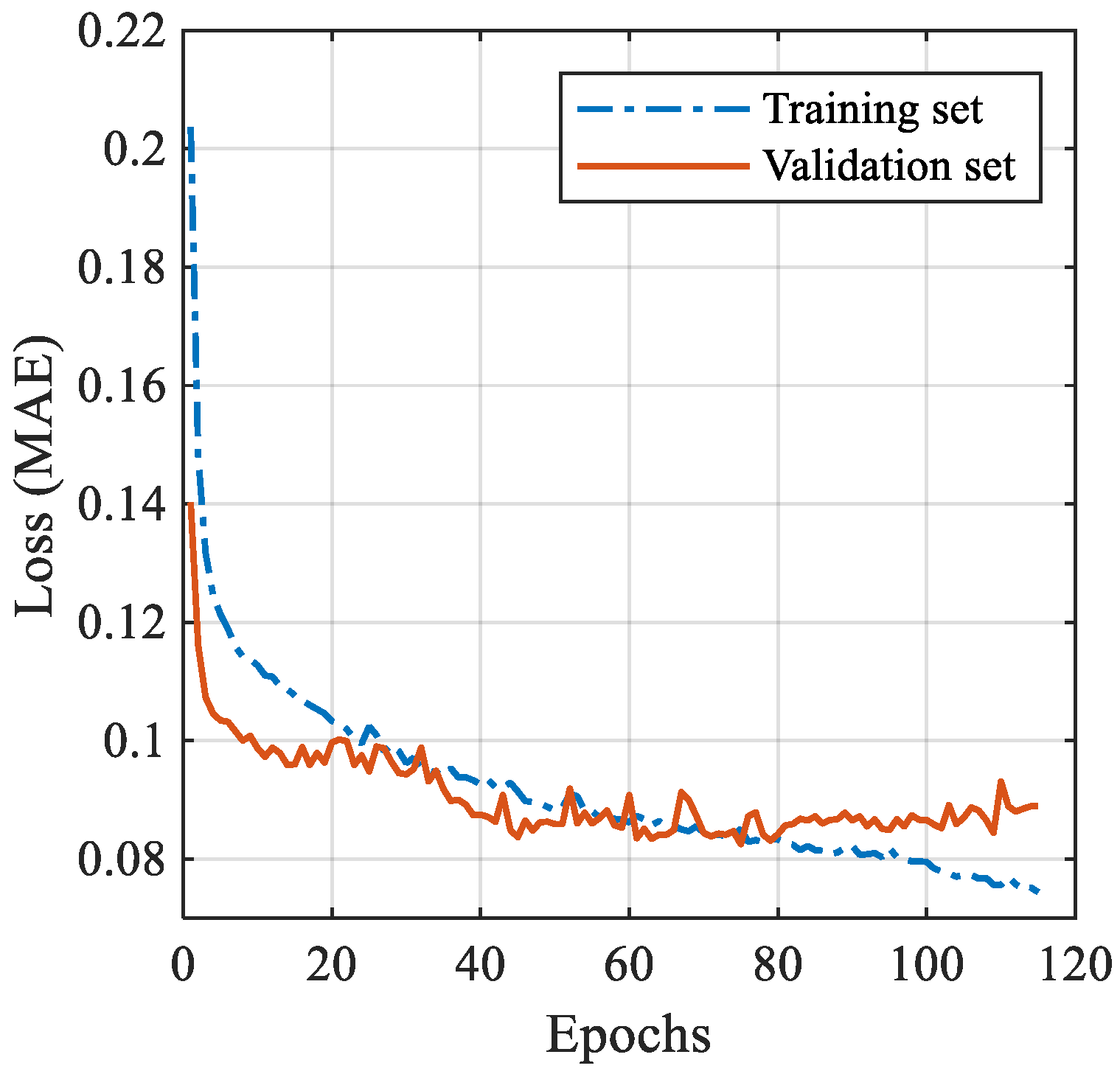
The training of the CNN adopts the EarlyStopping function [47]. The loss history of training and validation are shown in Figure 13. The results show that at the beginning of training, with the increase of epoch, the loss of training decreases rapidly. Subsequently, the loss of validation reaches the minimum (MAE = 0.0825) when the epoch is 75, and the program stopped training at the end of the 115th epoch. The prediction based on the CNN model takes 0.762 s using a laptop platform (i5-4210H, RAM 8G, GTX 960M), which is over 650 times faster than that using the THA-based method (507.81 s).
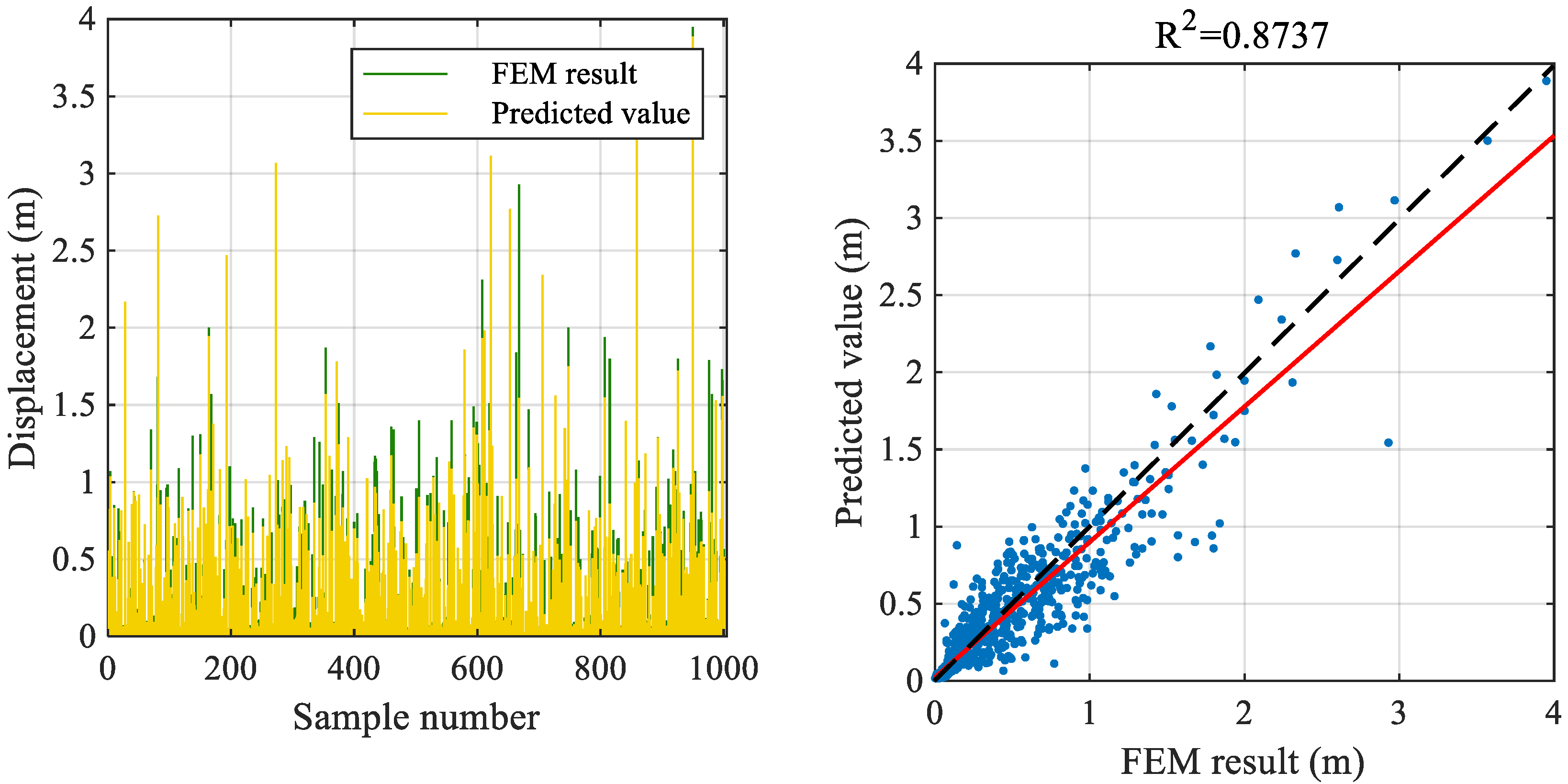
The test set is input into the optimal model, and the prediction result is shown in Figure 14 and Table 4. As evident in the result, the CNN model exhibits a good prediction accuracy, which outperforms the BPNN model (Figure 11). LeCun et al. [14] mentioned that conventional machine learning techniques (such as the BPNN used in this study) have limitations in processing raw forms of natural data. Therefore, build pattern recognition and machine learning system requires considerate and comprehensive engineering design of the feature extractor, which converts the raw data into a suitable internal representation or feature vector. When the feature extractor is not effective, the BPNN can learn very limited information. The CNN model, on the other hand, can extract more representative features of raw material through the training process, which can be used to solve more complex problems. Therefore, to further demonstrate the feature extraction process of the proposed CNN model, the visualization of extracted features in convolutional layers is discussed in the following section.

5.3. Feature Visualization of the CNN

As mentioned earlier, the CNN has better feature extraction performance compared with the BPNN. The CNN can directly extract effective features from ground motion data and avoid information loss caused by manual feature extraction. The convolutional layer extracts various features from the previous layer, and the pooling layer makes features robust to noise and deformation [14].
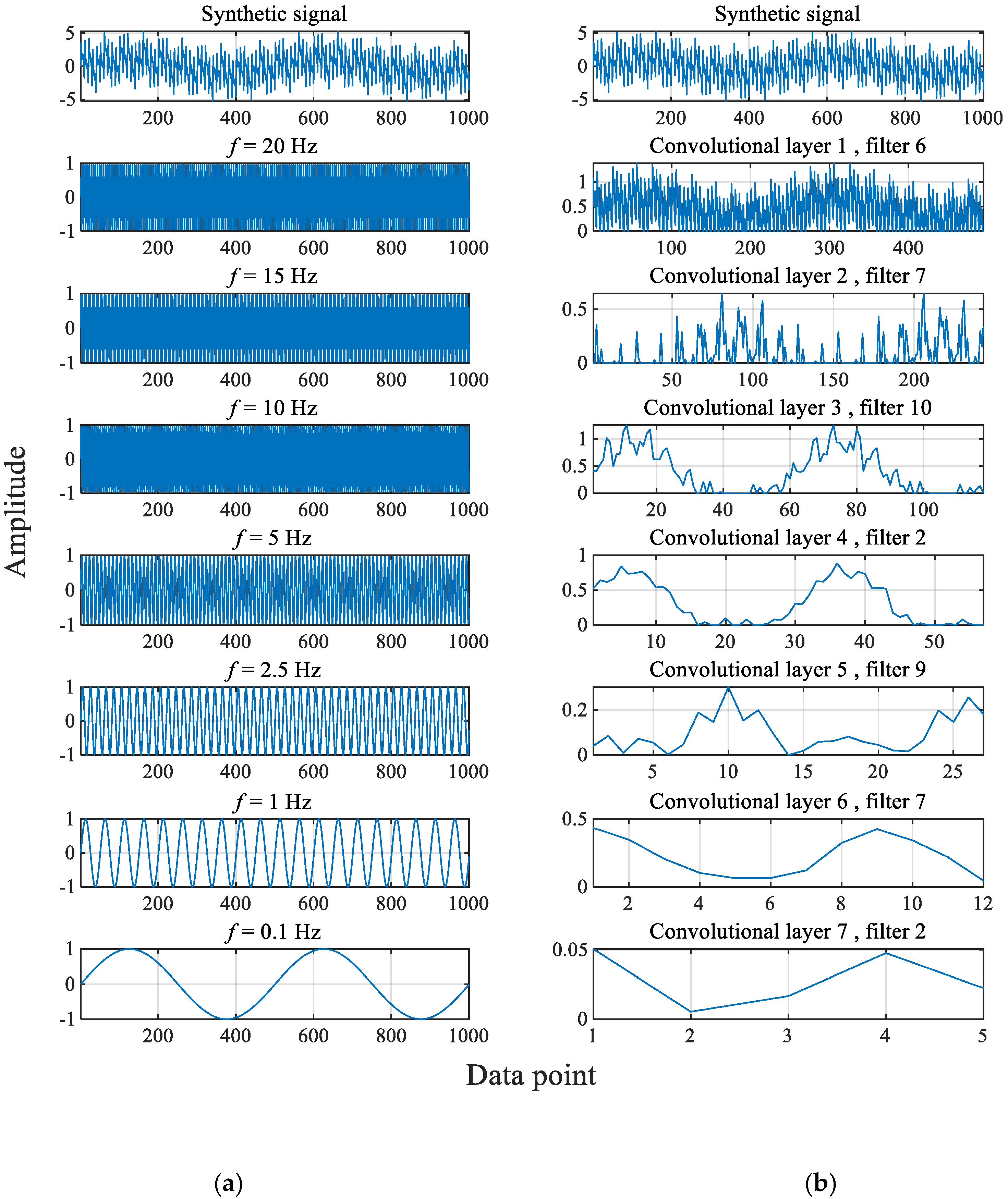
Visualizing the output of each convolutional layer (including the process of convolution and pooling) is helpful to understand the features extraction mechanism of the CNN. To clearly demonstrate the extracted feature of each convolutional layer, a synthetic signal is input into the CNN model. The synthetic signal is composed of seven simple harmonics with frequencies range from 0.1–20 Hz (Figure 15a). The output of each convolutional layer is presented in Figure 15b.
As shown in the right-hand side of Figure 15, the output of the first convolutional layer is similar to the synthetic signal, which not only capture the high-frequency features, but also carries the information of the overall trend (low-frequency). With the increase of convolution depth, the length of output data decreases continuously, and the proportion of low-frequency content increases gradually. For example, the result of the convolutional filter No. 2 in the fourth convolutional layer is very similar to the shape of the simple harmonic with the frequency of 0.1 Hz. The above results show that the shallow convolutional layers of the CNN model mainly extract the high-frequency features of a signal, while the deep convolutional layers primarily extract the low-frequency features of a signal. In addition, the features extracted by the CNN model can also reflect the time-domain features of a signal. Therefore, the CNN model can extract effective features of ground motions and yields better prediction than that of the BPNN model.
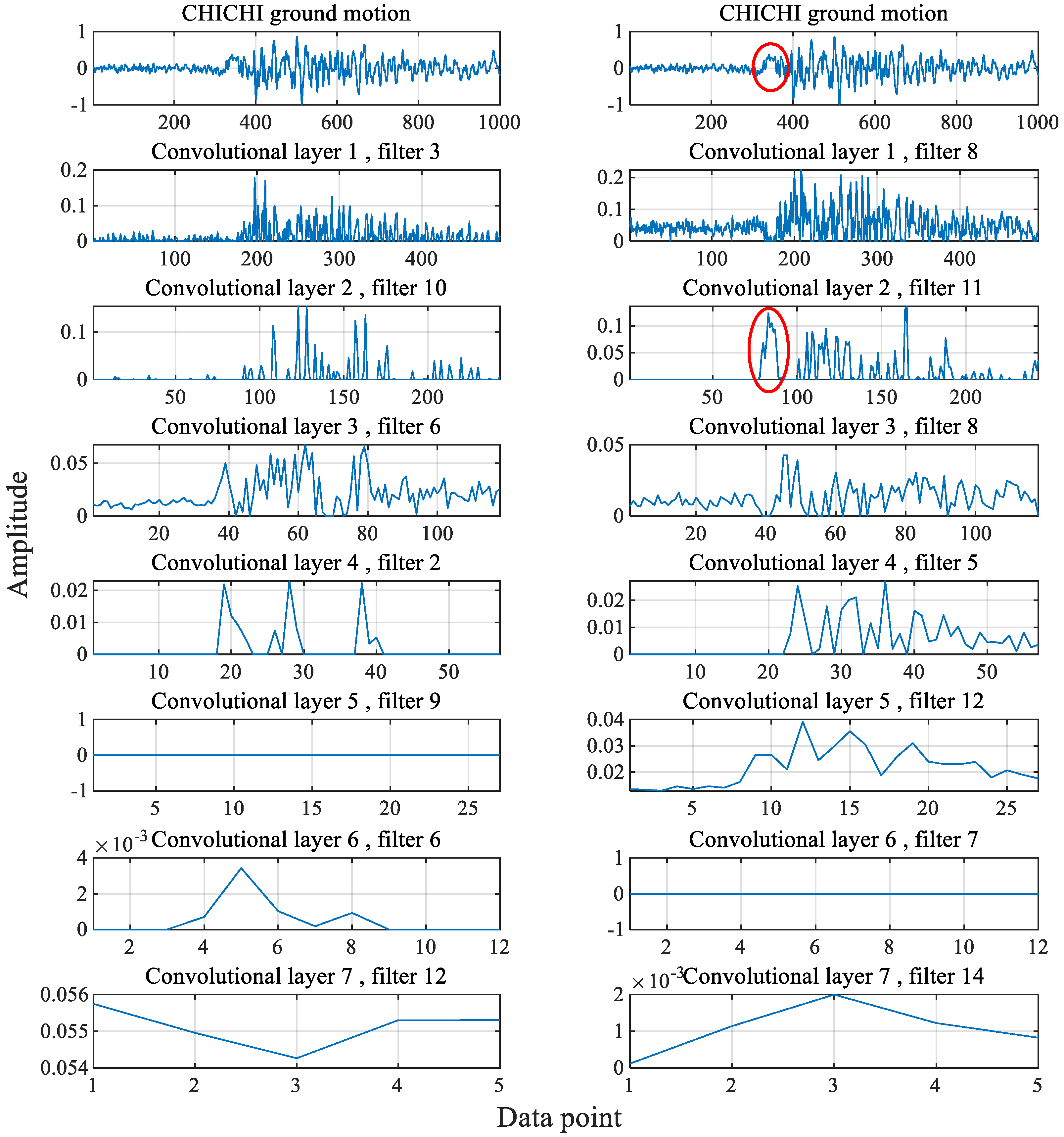
Subsequently, the Chichi05_CHY060-e ground motion (hereafter referred to as CHICHI) was input into the well-tuned the CNN model, and the outputs of seven convolutional layers are shown in Figure 16. Similar to the result of the synthetic signal, the outputs of shallow convolutional layers contain more high-frequency information. As the convolutional layer deep in, the outputs contain more low-frequency information. For example, in Figure 16, filter No. 11 of the second convolutional layer can well capture the location and shape of the feature in the red circles.
It is worth mentioning that the output of filter No. 9 in the fifth convolutional layer is null, which means this ground motion does not contain the corresponding feature. Because the CNN model is learning from a large number of ground motions, and different ground motions are so random that a feature extracted from one ground motion may not necessarily exist in another. This is why multiple filters are adopted in each convolutional layer of the CNN model. Multiple filters enable the model of learning more information on different ground motions and improve the generalization of the model.

6. Conclusions

In this study, a machine learning-based destructive power assessment method of earthquake to structures is proposed. The method is proposed based on the backpropagation neural network (BPNN) and convolutional neural network (CNN). The results of 50,570 numerical simulations are used as samples to train the machine learning models, and some conclusions can be drawn as follow:
  • For the feature extraction of ground motion time-history data, STFT can well reflect the frequency-/time-domain features of ground motions. The prediction using STFT as feature extractor yield higher accuracy (R2 = 0.6784) than that using FFT (R2 = 0.4277).
  • The selection of the number of layers and nodes of the BPNN is related to the features. In this study, in the case of 40 features as input, the optimal model is the BPNN with two hidden layers and three nodes in each layer. For the case of 10 features as input, the optimal model is the BPNN with two hidden layers and four nodes in each layer.
  • The model based on the CNN exhibits better prediction accuracy (R2 = 0.8737) than the BPNN model (R2 = 0.6784). This is because the convolution layer of the CNN can identify the frequency-/time-domain information of a signal, and avoid the bias caused by artificial feature extraction in the meantime. The advantage of the CNN is magnified for its deep network architecture and multiple filters in each layer.
  • Feature visualization of convolutional layers reveals that the shallow convolutional layers of the CNN model mainly extract the high-frequency features of a signal, while the deep convolutional layers primarily extract the low-frequency features of a signal. In addition, the features extracted by the CNN model can reflect the time-domain features of a signal.
  • The CNN model exhibits remarkable computational efficiency compared with THA-based method. For example, using a laptop platform (i5-4210H, 8G of RAM, GTX 960M), the prediction of 1000 structures using the CNN model takes 0.762 s, which is over 650 times faster than that using the THA-based method (507.81 s). The high computational efficiency of the CNN-based seismic response prediction makes it promising for use in the timely assessment of regional structures.
The research proves that the CNN model can make a significantly faster prediction of engineering demand parameters compared with THA-based method. The predicted engineering demand parameters can be used to assess the damage, economic loss, and downtime of regional structures based on damage assessment methods [9,56], to assist in emergency response and rapid disaster relief.

Author Contributions

Conceptualization, C.X.; Data curation, R.Z.; Funding acquisition, C.X.; Investigation, R.Z., X.D. and Q.L.; Methodology, R.Z. and C.X.; Project administration, C.X.; Resources, C.X. and Y.L.; Software, R.Z. and C.X.; Supervision, C.X. and Y.L.; Writing–original draft, R.Z. and C.X.; Writing–review & editing, R.Z., C.X., X.D. and Q.L. All authors have read and agreed to the published version of the manuscript.

Funding

This research was funded by National Key Research and Development Program (Grant No. 2019YFC1511003), Intellectual Innovation Program of Shenzhen Science and Technology Innovation Committee (Grant No. JCYJ20180305123919731) and National Natural Science Foundation of China (Grant No. 51708361).

Conflicts of Interest

The authors declare no conflict of interest.

References

  1. Ye, L.; Lu, X.; Li, Y. Design objectives and collapse prevention for building structures in mega-earthquake. Earthq. Eng. Eng. Vib. 2010, 9, 189–199. [Google Scholar] [CrossRef]
  2. Gordon, P.; Richardson, H.W.; Davis, B. Transport-related impacts of the Northridge earthquake. J. Transp. Stat. 1998, 1, 21–36. [Google Scholar]
  3. Applied Technology Council (ATC). ATC-40: The Seismic Evaluation and Retrofit of Concrete Buildings; Applied Technology Council: Redwood, CA, USA, 1996. [Google Scholar]
  4. Federal Emergency Management Agency (FEMA). Multi-Hazard Loss Estimation Methodology Earthquake Model. HAZUS-MH 2.1 Technical Manual; Federal Emergency Management Agency: Washington, DC, USA, 2012.
  5. Lin, Y.; Chang, K.; Wang, Y. Comparison of displacement coefficient method and capacity spectrum method with experimental results of RC columns. Earthq. Eng. Struct. Dyn. 2003, 33, 35–48. [Google Scholar] [CrossRef]
  6. Tantala, M.W.; Nordenson, G.J.P.; Deodatis, G.; Jacob, K. Earthquake loss estimation for the New York City metropolitan region. Soil Dyn. Earthq. Eng. 2008, 28, 812–835. [Google Scholar] [CrossRef]
  7. Xiong, C.; Lu, X.; Guan, H.; Xu, Z. A nonlinear computational model for regional seismic simulation of tall buildings. Bull. Earthq. Eng. 2016, 14, 1047–1069. [Google Scholar] [CrossRef]
  8. Xiong, C.; Deng, X.; Liang, Y.; Li, Q.; Huang, J.; Lin, X.; Li, D. Regional seismic damage simulation of corroded RC frame structures: A case study of Shenzhen city. Appl. Sci. 2020, 10, 4818. [Google Scholar] [CrossRef]
  9. Xiong, C.; Huang, J.; Lu, X. Framework for city-scale building seismic resilience simulation and repair scheduling with labor constraints driven by time–history analysis. Comput. Aided Civ. Infrastruct. Eng. 2020, 35, 322–341. [Google Scholar] [CrossRef]
  10. Lu, X.; Mckenna, F.; Cheng, Q.; Xu, Z.; Mahin, S.A. An open-source framework for regional earthquake loss estimation using the city-scale nonlinear time history analysis. Earthq. Spectra 2020, 36, 806–831. [Google Scholar] [CrossRef]
  11. Xiong, C.; Lu, X.; Huang, J.; Guan, H. Multi-LOD seismic-damage simulation of urban buildings and case study in Beijing CBD. Bull. Earthq. Eng. 2019, 17, 2037–2057. [Google Scholar] [CrossRef]
  12. Lu, X.; Lu, X.; Guan, H.; Ye, L. Collapse simulation of reinforced concrete high-rise building induced by extreme earthquakes. Earthq. Eng. Struct. Dyn. 2013, 42, 705–723. [Google Scholar] [CrossRef] [Green Version]
  13. Krizhevsky, A.; Sutskever, I.; Hinton, G.E. ImageNet classification with deep convolutional neural networks. Commun. ACM 2017, 60, 84–90. [Google Scholar] [CrossRef]
  14. LeCun, Y.; Bengio, Y.; Hinton, G. Deep learning. Nature 2015, 521, 436–444. [Google Scholar] [CrossRef] [PubMed]
  15. Dankovičová, Z.; Sovák, D.; Drotár, P.; Vokorokos, L. Machine learning approach to dysphonia detection. Appl. Sci. 2018, 8, 1927. [Google Scholar] [CrossRef] [Green Version]
  16. Lee, J.; Park, J.; Kim, K.L.; Nam, J. SampleCNN: End-to-end deep convolutional neural networks using very small filters for music classification. Appl. Sci. 2018, 8, 150. [Google Scholar] [CrossRef] [Green Version]
  17. Xu, Z.; Wu, Y.; Qi, M.Z.; Zheng, M.; Lu, X. Prediction of structural type for city-scale seismic damage simulation based on machine learning. Appl. Sci. 2020, 10, 1795. [Google Scholar] [CrossRef] [Green Version]
  18. Mangalathu, S.; Heo, G.; Jeon, J.S. Artificial neural network based multi-dimensional fragility development of skewed concrete bridge classes. Eng. Struct. 2018, 162, 166–176. [Google Scholar] [CrossRef]
  19. Nguyen, H.; Moayedi, H.; Foong, L.K.; Al Najjar, H.A.H.; Jusoh, W.A.W.; Rashid, A.S.A.; Jamali, J. Optimizing ANN models with PSO for predicting short building seismic response. Eng. Comput. 2019, 36, 823–837. [Google Scholar] [CrossRef]
  20. Zhang, R.; Liu, Y.; Sun, H. Physics-guided convolutional neural network (PhyCNN) for data-driven seismic response modeling. Eng. Struct. 2020, 215, 110704:1–110704:13. [Google Scholar] [CrossRef]
  21. Kiani, J.; Camp, C.; Pezeshk, S. On the application of machine learning techniques to derive seismic fragility curves. Comput. Struct. 2018, 218, 108–122. [Google Scholar] [CrossRef]
  22. Xiong, C.; Li, Q.; Lu, X. Automated regional seismic damage assessment of buildings using an unmanned aerial vehicle and a convolutional neural network. Autom. Constr. 2020, 109, 102994:1–102994:14. [Google Scholar] [CrossRef]
  23. Mangalathu, S.; Sun, H.; Nweke, C.C.; Yi, Z.; Burton, H.V. Classifying earthquake damage to buildings using machine learning. Earthq. Spectra 2020, 36, 183–208. [Google Scholar] [CrossRef]
  24. Mangalathu, S.; Hwang, S.; Choi, E.; Jeon, J. Rapid seismic damage evaluation of bridge portfolios using machine learning techniques. Eng. Struct. 2019, 201, 109785:1–109785:12. [Google Scholar] [CrossRef]
  25. Zhang, R.; Chen, Z.; Chen, S.; Zheng, J.; Buyukozturk, O.; Sun, H. Deep long short-term memory networks for nonlinear structural seismic response prediction. Comput. Struct. 2019, 220, 55–68. [Google Scholar] [CrossRef]
  26. Hochreiter, S.; Schmidhuber, J. Long short-term memory. Neural Comput. 1997, 9, 1735–1780. [Google Scholar] [CrossRef] [PubMed]
  27. Zhang, Y.; Wang, C.; Gong, L.; Lu, Y.; Zhou, X. A Power-Efficient Accelerator Based on FPGAs for LSTM Network. In Proceedings of the IEEE International Conference on Cluster Computing 2017, Honolulu, HI, USA, 5–8 August 2017. [Google Scholar]
  28. Rumelhart, D.E.; Hinton, G.E.; Williams, R.J. Learning representations by back-propagating errors. Nature 1986, 323, 533–536. [Google Scholar] [CrossRef]
  29. Federal Emergency Management Agency (FEMA). NEHRP Guidelines for the Seismic Rehabilitation of Buildings: FEMA 273; Federal Emergency Management Agency (FEMA): Washington, DC, USA, 1997.
  30. Applied Technology Council (ATC). Earthquake Damage Evaluation Data for California. ATC-13 Report; Applied Technology Council: Redwood, CA, USA, 1985. [Google Scholar]
  31. Hiroshi, K.; Masaomi, T.; Norihide, K.; Hiroshi, I. Conversion of multi-story building into equivalent SDOF system and its predictability for earthquake response. J. Struct. Constr. Eng. 2001, 66, 79–85. (In Japanese) [Google Scholar] [CrossRef] [Green Version]
  32. Irie, T.; Mazda, T.; Sumaya, A.D. Application of an estimation method for response of structures by equilibrium energies. In Proceedings of the 12th World Conference on Earthquake Engineering (WCEE 2000), Auckland, New Zealand, 30 January–4 February 2000. [Google Scholar]
  33. PEER Center. PEER Ground Motion Database; PEER NGA-West2 Database 2013/03; Pacific Earthquake Engineering Research Center Headquarters at the University of California: Berkeley, CA, USA, 2013. [Google Scholar]
  34. Ng, A. The Deeplearning.ai Blog/BOOKS/Machine Learning Yearning. Available online: https://www.deepLearning.ai/machine-learning-yearing (accessed on 7 August 2020).
  35. Funahashi, K. On the approximate realization of continuous mappings by neural networks. Neural Netw. 1989, 2, 183–192. [Google Scholar] [CrossRef]
  36. Setti, S.; Rao, R. Artificial neural network approach for prediction of stress–strain curve of near β titanium alloy. Rare Met. 2014, 33, 249–257. [Google Scholar] [CrossRef]
  37. Corinthios, M.J. A fast fourier transform for high-speed signal processing. IEEE Trans. Comput. 1971, C-20, 843–846. [Google Scholar] [CrossRef]
  38. Fessler, J.A.; Sutton, B.P. Nonuniform fast Fourier transforms using min-max interpolation. IEEE Trans. Signal Proc. 2003, 51, 560–574. [Google Scholar] [CrossRef] [Green Version]
  39. Enochson, L.D.; Piersol, A.G. Application of fast Fourier transform procedures to shock and vibration data analysis. In Proceedings of the Aeronautic and Space Engineering Manufacturing Meeting, Los Angeles, CA, USA, 2–6 October 1967. [Google Scholar]
  40. Cooley, J.W.; Lewis, P.A.W.; Welch, P.D. The fast Fourier transform and its applications. IEEE Trans. Educ. 1969, 12, 27–34. [Google Scholar] [CrossRef] [Green Version]
  41. Petrellis, N. Undersampling in orthogonal frequency division multiplexing telecommunication systems. Appl. Sci. 2014, 4, 79–98. [Google Scholar] [CrossRef]
  42. Ho, T.-J.; Chung, M.-J. Information-aided smart schemes for vehicle flow detection enhancements of traffic microwave radar detectors. Appl. Sci. 2016, 6, 196. [Google Scholar] [CrossRef] [Green Version]
  43. Xu, P.; Xiao, C.; Li, J. Research on relationship between natural vibration periods and structural heights for high-rise buildings and its reference range in China. Int. J. High Rise Build. 2014, 3, 49–64. [Google Scholar] [CrossRef]
  44. Gu, Y.H.; Bollen, M.H.J. Time-frequency and time-scale domain analysis of voltage disturbances. IEEE Trans. Power Deliv. 2000, 15, 1279–1284. [Google Scholar] [CrossRef]
  45. Atiya, A.; Ji, C. How initial conditions affect generalization performance in large networks. IEEE Trans. Neural Netw. 1997, 8, 448–451. [Google Scholar] [CrossRef] [Green Version]
  46. Drucker, H.; Le Cun, Y. Improving generalization performance using double backpropagation. IEEE Trans. Neural Netw. 1992, 3, 991–997. [Google Scholar] [CrossRef]
  47. Nair, V.; Hinton, G.E. Rectified linear units improve restricted boltzmann machines. In Proceedings of the 27th International Conference on Machine Learning, Haifa, Israel, 21–24 June 2010; pp. 807–814. [Google Scholar]
  48. Williams, P. Bayesian regularization and pruning using a Laplace prior. Neural Comput. 1995, 7, 117–143. [Google Scholar] [CrossRef]
  49. Masood, S.; Doja, M.N.; Chandra, P. Analysis of weight initialization methods for gradient descent with momentum. In Proceedings of the 2015 International Conference on Soft Computing Techniques and Implementations(ICSCTI), Faridabad, India, 8–10 October 2015; pp. 131–136. [Google Scholar]
  50. Yao, Y.; Rosasco, L.; Caponnetto, A. On early stopping in gradient descent learning. Constr. Approx. 2007, 26, 289–315. [Google Scholar] [CrossRef]
  51. Sujadevi, V.G.; Soman, K.P.; Vinayakumar, R.; Sankar, A.U.P. Anomaly detection in phonocardiogram employing deep learning. Comput. Intell. Data Min. 2019, 711, 525–534. [Google Scholar] [CrossRef]
  52. Raza, A.; Mehmood, A.; Ullah, S.; Ahmad, M.; Choi, G.S.; On, B.-W. Heartbeat Sound Signal Classification Using Deep Learning. Sensors 2019, 19, 4819. [Google Scholar] [CrossRef] [PubMed] [Green Version]
  53. LeCun, Y.; Bottou, L.; Bengio, Y.; Haffner, P. Gradient-based learning applied to document recognition. Proc. IEEE. 1998, 86, 2278–2324. [Google Scholar] [CrossRef] [Green Version]
  54. Simonyan, K.; Zisserman, A. Very deep convolutional networks for large-scale image recognition. In Proceedings of the International Conference on Learning Representations 2015 (ICLR 2015), San Diego, CA, USA, 7–9 May 2015. [Google Scholar]
  55. Kingma, D.P.; Ba, J.L. Adam: A method for stochastic optimisation. arXiv 2014, arXiv:1412.6980. [Google Scholar]
  56. Federal Emergency Management Agency (FEMA). Seismic Performance Assessment of Buildings Volume 1—Methodology; Technical Report FEMA-P58; Federal Emergency Management Agency: Washington, DC, USA, 2012.
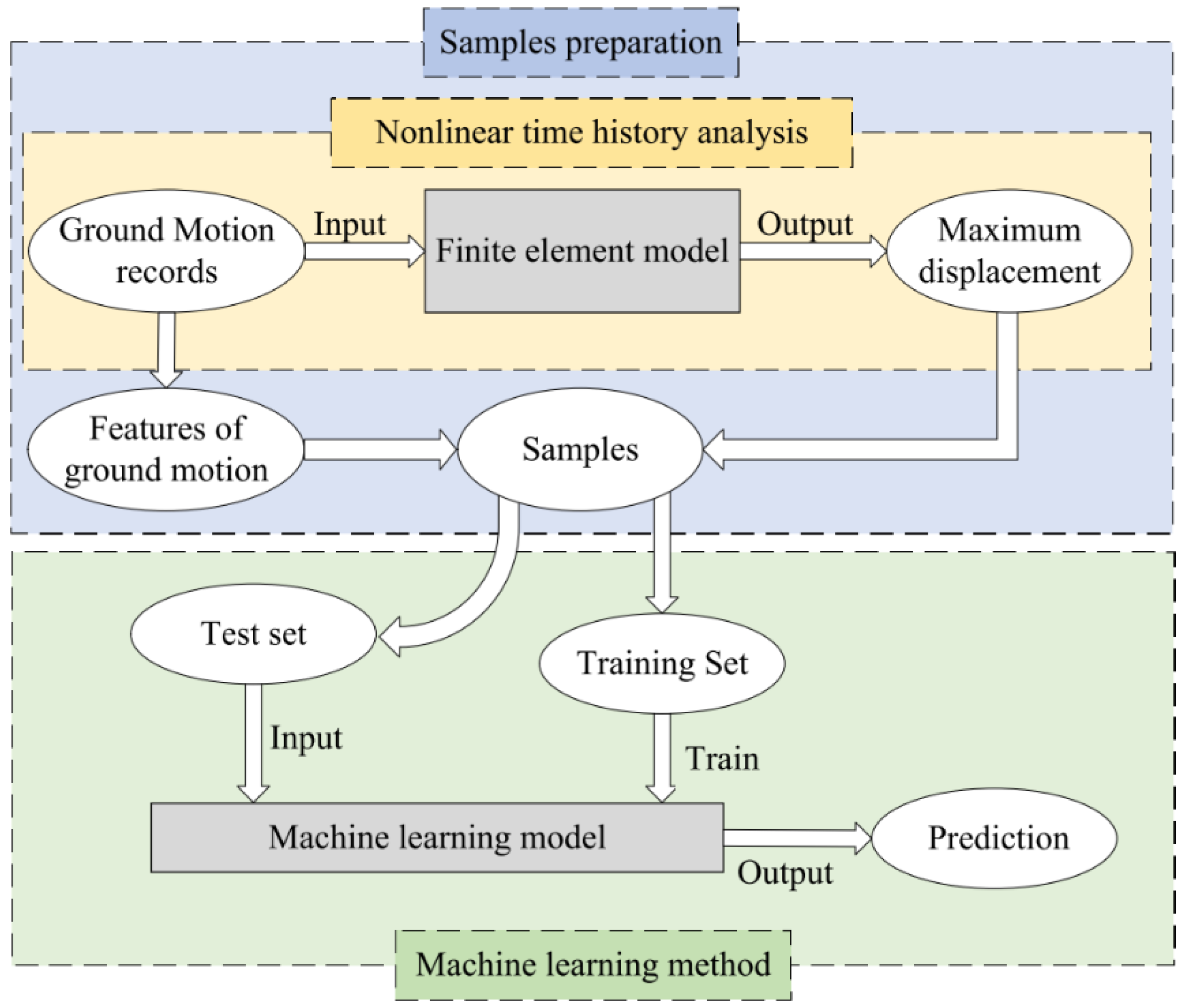
Figure 1. Analysis procedure of the proposed method.
Applsci 10 06210 g001
Figure 2. Single degree-of-freedom (SDOF) shear model: (a) SDOF shear model; (b) tri-linear backbone curve; (c) single-parameter hysteretic model.
Applsci 10 06210 g002
Figure 3. Acceleration response spectra of partial ground motions.
Applsci 10 06210 g003
Figure 4. Comparison of ground motions: (a) Acceleration time histories; (b) acceleration response spectra; (c) frequency spectra.
Applsci 10 06210 g004
Figure 5. Forty feature values of ground motions: (a) Features of 0~5 s time interval; (b) features of 5~10 s time interval; (c) features of 10~15 s time interval; (d) features of 15~20 s time interval.
Applsci 10 06210 g005
Figure 6. Ten feature values of ground motions.
Applsci 10 06210 g006
Figure 7. Optimization of the BPNN structure (40 feature values): (a) R2 of validation set (one hidden layer); (b) mean absolute error (MAE) of validation set (one hidden layer); (c) R2 of validation set (two hidden layers); (d) MAE of validation set (two hidden layers).
Applsci 10 06210 g007
Figure 8. Optimization of the BPNN structure (10 feature values): (a) R2 of validation set (one hidden layer); (b) MAE of validation set (one hidden layer); (c) R2 of validation set (two hidden layers); (d) MAE of validation set (two hidden layers).
Applsci 10 06210 g008
Figure 9. Feature extraction and network architecture.
Applsci 10 06210 g009
Figure 10. Loss (MAE) history of the BPNN.
Applsci 10 06210 g010
Figure 11. Test results of the BPNN model: (a) Test results of the BPNN based on the STFT features; (b) Test results of the BPNN based on FFT features.
Applsci 10 06210 g011
Figure 12. The architecture of the adopted the CNN model.
Applsci 10 06210 g012
Figure 13. Loss (MAE) history of the CNN.
Applsci 10 06210 g013
Figure 14. Test results of the CNN model.
Applsci 10 06210 g014
Figure 15. Comparison of synthetic signal components and extracted features: (a) Synthetic signal and its simple harmonic components; (b) features extracted from different convolutional layers.
Applsci 10 06210 g015
Figure 16. Features extracted from different convolutional layers.
Applsci 10 06210 g016
Table 1. Comparison of machine learning-based seismic response simulation methods. LSTM, long-short-term memory; BPNN, backpropagation neural network; CNN, convolutional neural network; EDP, engineering demand parameters.
LiteraturesSimulation OutputsProblem TypeComputational WorkloadMachine Learning Methods
Mangalathu et al. [23,24]Structural damage statesClassificationLightDiscriminant analysis, k-nearest neighbors, decision trees, random forests
Zhang et al. [25]Structural time-history responseTime series predictionModerateLSTM network
This studyEDPValue predictionLightBPNN, CNN
Table 2. Structural parameters of the elasto-plastic SDOF model.
Natural Period (s)Damping RatioYield Strength to Weight RatioPeak to Yield Strength RatioSecondary Stiffness RatioHysteretic Parameter
0.50.050.0972.610.250.4
Table 3. Statistical indexes of prediction results. STFT, short-time Fourier transform; FFT, fast Fourier transform.
Feature Extraction MethodMAEMSERMSER2
STFT0.14990.08130.28520.6784
FFT0.24360.09380.30630.4277
Table 4. Statistical indexes of prediction result.
MAEMSERMSER2
0.08830.02630.16210.8737