Effects of Inclination Angles on Stepped Chute Flows

Abstract

Owing to its effective energy dissipation and aeration, a stepped spillway is commonly used for flood release in hydraulic projects. Its conventional design features horizontal step surfaces. Designed for certain flow rates, it does not function satisfactorily at larger discharges. To improve this, layouts with inclined step surfaces, both downward and upward, are proposed. Computational fluid dynamics (CFD) modelling in 3D is performed to examine and compare their flow properties in the skimming flow. The results suggest that a shift from a downward to an upward layout leads to a gradual decrease in the flow velocity at the chute end; the latter exhibit higher energy dissipation efficiency. Moreover, equations are developed to estimate the velocity and energy loss. The flow velocity in the developing zone, described by a power law, shows a decline with an increase in the angle of inclination. The downward layout is subjected to somewhat higher risk of cavitation if implemented in a prototype. The extreme pressure loads acting upon an upward layout are larger, and a correlation is proposed for its prediction. On an inclined surface, either upward or downward, the pressure demonstrates an S-shaped distribution. On a vertical surface, the flow pressure increases, after an initial decline over a short distance, towards the chute bottom.

1. Introduction

A spillway is a flood discharge structure that has been applied in hydropower and irrigation projects for decades. Particularly, in the area with narrow river width, a stepped spillway is an alternative to a large energy dissipater [1]. The steps act as roughness elements and heighten the bottom friction, thanks to which more kinetic energy is dissipated in comparison with the smooth layout. As a result, the required extent of the downstream energy dissipation arrangement is reduced, leading to lower total engineering costs [2]. In addition, owing to the advances in roller-compacted concrete (RCC) techniques, stepped chutes have, over the past decades, found wide applications in handling extreme floods [3].

Despite the advantages, traditional stepped spillways are, in certain situations, insufficient to effectively dissipate energy and prevent cavitation risk. In countries including Sweden, the criteria for design-flood determinations for dams are re-evaluated; new flood guidelines have come into force [4]. For many existing dams, this leads to higher flood magnitudes, which requires that the spillway discharge capacity should be enlarged. Another contributing factor is the climate changes. Improved spillway design is necessary to meet the new flood standards.

Zhang and Chanson examined the air–water properties on a stepped spillway with modified steps and cavities [5]. It was concluded that partial cavity blockages have little effect on air entrainment, but were linked to an increased presence of large-scale structures in the overflow. Ghaderi et al. performed numerical simulations on a spillway with trapezoidal labyrinth-shaped steps [6]. Relative to the conventional layout, a lower residual head and a larger friction factor were found in the labyrinth one. Wüthrich and Chanson proposed a stepped chute formed with gabions [7]. Compared with a layout with smooth surface, it led to less air entrainment and lower turbulence intensity. Felder and Chanson conducted model tests on a pooled stepped spillway and examined its two-phase air–water flow properties [8]. Gonzalez and Chanson performed experiments of a large stepped chute equipped with triangular vanes and longitudinal ribs [9]. In comparison with the conventional one, larger flow resistance and more energy dissipation are evidenced. In a chute with upward inclined steps, Chinnarasri and Wongwises looked into its flow regimes and proposed an empirical formula for energy loss prediction [10].

The focus of the previous investigations is mainly on examinations of energy loss in stepped chutes. Though the studies are fewer in number, they contribute to the understanding of the importance of step layouts. Despite this, insights into the step effects and cavitation behaviors are limited. Based on the geometrical layout of a stepped chute spillway examined elsewhere, CFD modelling in 3D is made, with emphasis on the step angling of the horizontal surfaces. With several typical layouts included, the study examines the characteristics of flow pressure and velocity and illustrate their differences in cavitation potential. The purpose is to identify their pros and cons, evaluate their suitability and provide guidance for improved step design in engineering applications. The upward layout is found an effective alternative to improve energy dissipation and mitigate cavitation risks.

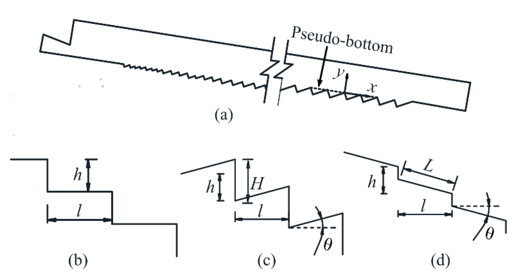
2. Geometrical Layout of Steps

Bai et al. [11] performed both numerical modelling and laboratory tests, and documented the hydraulic properties of flows in a stepped spillway with both V-shaped and conventional steps. It is the latter that is adopted in this study. By conventional steps, we mean steps of rectangular shape (Figure 1a,b).

In their studies, a sufficiently large water tank conveys water to the test rig. On one side of the tank, an overflow weir is installed to guarantee constant water stage at a given flow rate. From the tank, the water flows, via a short conduit, into the spillway chute, with a width B = 0.40 m. The conduit is rectangular in cross-section, converging vertically and covering the whole flume width. The downstream cross-section of the conduit, where the flow transits from pressurized to free surface, is at a 0.80 m distance from the first step and 0.12 m in height (measured perpendicular to the flume bottom). The spillway chute has a slope of φ = 26.6° and 56 steps. It features two types of steps, first with 28 transitional steps of a linearly enlarged step size and then with 28 major steps of a constant step dimension. Let h and l denote step height and length. From the twenty-ninth step and downward, h = 0.06 m and l = 0.12 m. This longitudinal step layout is maintained in the study.

Let θ be the inclination angle (in degree) of step surfaces with the horizontal. Five geometrical layouts are devised through changes in the step angling, i.e., θ = −20°, −10°, 0°, 10° and 20°. A positive and negative θ value denotes an upwards and downwards sloping surface, respectively (Figure 1c,d). For the conventional steps, θ = 0°. The equivalent step height is defined as H = h + l × tanθ; the equivalent step surface length is L = l/cosθ. The range of H = 0.016–0.104 m and L = 0.120–0.108 m. The pseudo-bottom refers to the straight line running through the step vertices (Figure 1). An x-y coordinate system is also set up. The x-axis coincides with the pseudo-bottom; the perpendicular y-axis has its origin on it. The layouts are simulated to look into the effects of θ on hydraulic behaviors expressed in terms of flow velocity, flow pressure and energy dissipation.

3. Numerical Simulations

CFD modelling is performed of the two-phase flows of water and air in the flume. The k-ε turbulence model and the volume of fluid (VOF) method are combined to reproduce the flow features. The simulations are made in three dimensions, covering the whole flume width.

3.1. Turbulence Model

Free-surface flows in a stepped spillway feature high turbulence intensity and air entrainment. A proper numerical model is essential to obtain reasonable simulation results. Investigations [12,13,14] show that the k-ε turbulence model is suitable for simulations of the spillway flows. Bai et al. [11] used this model in examinations of the flow and pressure field in the conventional stepped spillway (θ = 0). Thus, this model is used to reproduce the hydraulic features of the proposed layouts. The governing equations read:

The turbulence kinetic energy (k) equation:

$$\frac{\partial \left(\rho k\right)}{\partial t}+\frac{\partial }{\partial x_i}\left(\rho u_{i}k\right)=\frac{\partial }{\partial x_i}\left[\left(\mu +\frac{{\mu }_t}{{\sigma }_k}\right)\frac{\partial k}{\partial x_i}\right]+G_k+G_b-\rho \epsilon -Y_M+S_k$$

(1)

The turbulence kinetic energy dissipation rate (ε) equation:

$$\frac{\partial \left(\rho \epsilon \right)}{\partial t}+\frac{\partial \left(\rho u_i\epsilon \right)}{\partial x_i}=\frac{\partial }{\partial x_i}\left[\left(\mu +\frac{{\mu }_t}{{\sigma }_{\epsilon }}\right)\frac{\partial \epsilon }{\partial x_i}\right]+C_{1\epsilon }\frac{\epsilon }{k}\left(G_k+G_{3\epsilon }{G}_b\right)-C_{2\epsilon }\rho \frac{{\epsilon }^2}{k}+S_{\epsilon }$$

(2)

where ρ = flow density, u_i = velocity component, t = time, μ = dynamic viscosity, μ_t = turbulent dynamic viscosity, G_k = generation of turbulent kinetic energy due to mean velocity gradients, G_b = generation of turbulent kinetic energy due to buoyancy, Y_M = contribution of the fluctuating dilatation in compressible turbulence to the overall dissipation rate, σ_k, σ_ε = turbulent Prandtl numbers for k and ε, and S_k and S_ε = user-defined source terms. The model constants are C_μ = 0.09, σ_k = 1.0, ε = 1.3, C_1ε = 1.44, C_2ε = 1.92 and C_3ε = 1.0. Although Longo et al. [15] and Di Federico et al. [16] suggested that model sensitivity be tested, the often-used default settings are adopted in the model.

In combination with the k-ε model, the VOF method is employed to track air–water interfaces with the geometric reconstruction scheme

$$\frac{\partial {\alpha }_w}{\partial t}+\frac{\partial \left({\alpha }_w{u}_i\right)}{\partial x_i}=0$$

(3)

The continuity and momentum equations are

$$\frac{\partial \rho }{\partial t}+\frac{\partial \rho u_i}{\partial x_i}=0$$

(4)

$$\frac{\partial \rho u_i}{\partial t}+\frac{\partial \rho u_i{u}_j}{\partial x_j}=-\frac{\partial P}{\partial x_i}+\frac{\partial }{\partial x_j}\left(\mu +{\mu }_t\right)\left(\frac{\partial u_i}{\partial x_j}+\frac{\partial u_j}{\partial x_i}\right)$$

(5)

where u_j = velocity component, α_w = volume fraction of water and P = pressure. The max. and min. values of α_w are 1 and 0, corresponding to full water and only air in a cell, respectively.

The simulations are performed in ANSYS Fluent. Based on the finite-volume method, the governing equations are solved with the SIMPLE algorithm for the coupling of pressure and velocity. The least-square cell-based method models the gradient. For solutions of P and α_w, the PRESTO! and Geo-Reconstruct techniques are used. The second-order upwind scheme is applied for the momentum; the first-order upwind scheme for the turbulent kinetic energy and dissipation rate.

3.2. Boundary and Flow Conditions

As described above, the flow transits from pressurized to free surface in the upper flume. The starting cross-section of the pressurized flow forms the upstream boundary of the computational domain. Downstream, the domain ends up with a cross-section (exit) 0.4 m from the last step (i.e., step no. 56). The drop height from the inlet to the outlet is H_T ≈ 3.0 m. The domain’s upper boundary is parallel to the chute bottom and well above the water surface. The whole flume width is included in the domain.

The 3D domain is meshed with structural grids. The upstream inlet is set as water velocity inlet, at which the turbulence conditions are expressed in terms of turbulence intensity level and turbulence viscosity ratio. Their embedded values in the program are 3% and 5, respectively, which are typical for flume inlet conditions [17]. The downstream and upper boundaries are defined as pressure outlet. The flume bottom and sidewalls are treated as solid wall.

Five flow rates are examined in the study (i.e., Q = 124.77 to 239.57 L/s). The corresponding unit discharge q = Q/B = 0.31–0.60 m²/s. The inlet water velocity V_in = 2.6–5.0 m/s, Froude number F = 4.41–8.47, and Reynolds number R = (1.19–2.28) × 10⁵.

3.3. Grid-Independent Solution

The simulations are made in 3D. The discretization error is a factor affecting the accuracy of CFD modelling. To produce grid-independent results, the grid reliability must be checked on the basis of grid density. The grid convergence index (GCI) method is used to estimate the discretization error [18], achieved in the steps that follow:

1.

Let n denote cell number of the domain. Generate, for a 3D domain, three grids with n cells and calculate their reprehensive grid size (S)

$$S={\left[\frac{1}{n}{\displaystyle \sum _{i=1}^n\Delta V_i}\right]}^{1/3}$$

(6)

where $\Delta V_i$ = cell volume.

2.

Calculate apparent order p,

$$p=\frac{1}{\ln \left(r_{21}\right)}\left|\ln \left|{\epsilon }_{32}/{\epsilon }_{21}\right|+\ln \left(\frac{r_{21}^p-\mathrm{sgn}\left({\epsilon }_{32}/{\epsilon }_{21}\right)}{r_{32}^p-\mathrm{sgn}\left({\epsilon }_{32}/{\epsilon }_{21}\right)}\right)\right|$$

(7)

where ${\varphi }_{i=1,2,3}$ = solutions by different grids, ${\epsilon }_{21}={\varphi }_2-{\varphi }_1$, ${\epsilon }_{32}={\varphi }_3-{\varphi }_2$, $r_{21}=S_2/S_1$, and $r_{32}=S_3/S_2$. The refinement is made around the steps, with refinement factor S_coarse/S_fine = 1.31.

3.

Determine the GCI,

$$\mathrm{GCI}=\frac{1.25\left|\left({\varphi }_1-{\varphi }_2\right)/{\varphi }_1\right|}{{\left(S_2/S_1\right)}^p-1}$$

(8)

In the study, n = 1.00, 0.68 and 0.30 million. Define V = flow velocity, V_max = max. velocity, g = gravitational acceleration, and d_c = (q²/g)^1/3 = critical flow depth, two dimensionless parameters, V/V_max and P/(ρgd_c), are selected to check the grid independence.

Table 1. Showcased calculations of grid convergence index (GCI) in P/(ρgd_c).

	X/L = 0.10	X/L = 0.25	X/L = 0.40	X/L = 0.60
r21	1.14	1.14	1.14	1.14
r32	1.31	1.31	1.31	1.31
ϕ1	0.0926	−0.0663	0.1066	0.6643
ϕ2	0.0933	−0.0658	0.1063	0.6644
ϕ3	0.0928	−0.0661	0.1086	0.6675
p	0.63	1.38	1.33	0.85
GCI (%)	10.68	4.00	1.70	0.04

and

Table 2. Showcased calculations of GCI in V/V_max.

	y/ymax = 0.2	y/ymax = 0.4	y/ymax = 0.6	y/ymax = 0.8
r21	1.14	1.14	1.14	1.14
r32	1.31	1.31	1.31	1.31
ϕ1	0.5807	0.7790	0.9007	0.9719
ϕ2	0.5818	0.7797	0.9011	0.9721
ϕ3	0.5813	0.7792	0.9007	0.9719
p	2.55	0.70	0.08	0.04
GCI (%)	0.57	1.03	4.42	2.60

show the discretization errors in terms of P/(ρgd_c) and V/V_max, respectively. Let S₁ < S₂ < S₃; define r₂₁ = S₂/S₁ and r₃₂ = S₃/S₂. Let X be the distance along an inclined step face, with its origin at the step corner, X/L = 1.0 corresponding to the step vertex, and y_max = the maximum value of y. Four X locations are selected to check GCI. The results show that the GCI values are below 4.5% for V/V_max at all locations and 4% for P/(ρgd_c) except for at X/L = 0.10. The differences between the three grids are insignificant. For the sake of the computational efficiency, the medium-sized grid with n = 0.68 million is chosen.

4. Results and Analysis

Depending on flow conditions, the flow over a stepped spillway is usually categorized into three regimes: nape, transition and skimming [19,20]. In engineering practice, the skimming flow regime is more relevant than the other two [21,22]. In the present study, skimming flows occur at all discharges. R varies within the range (1.19–2.28) × 10⁵, implying that the viscous effects can be neglected [11]. Simulations of the whole flume width are made. The results show; however, the flows are predominantly two-dimensional. At a given step, the central part of the transverse flow sees hardly any changes in, for example, velocity and pressure. Therefore, the discussions are based on the results along the chute’s symmetry plane. The effects of the step angling on the flow are evaluated in terms of velocity distribution, flow pressure and efficiency of energy dissipation.

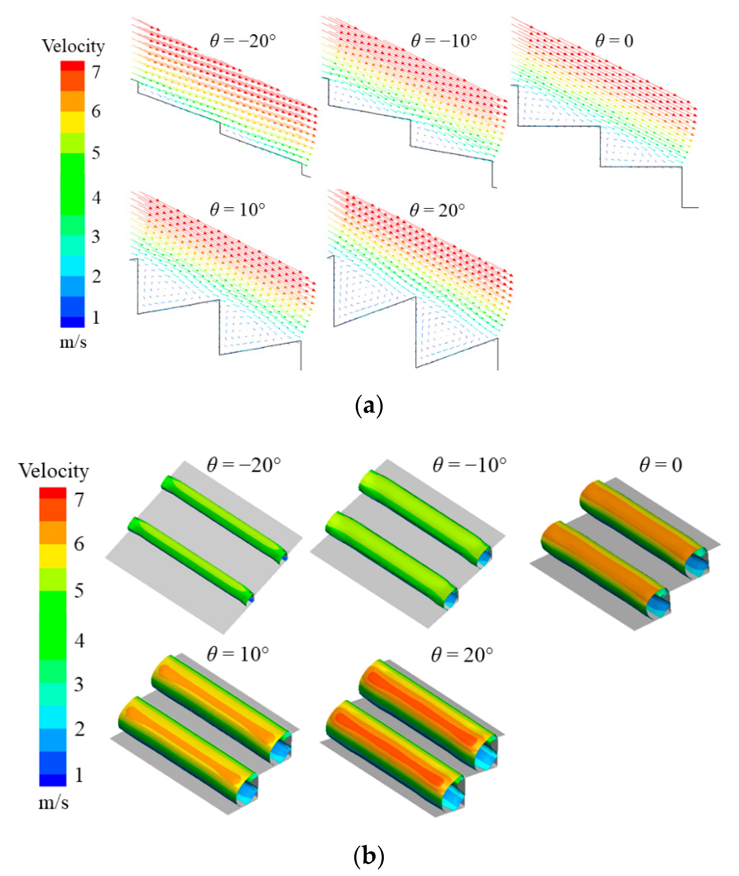
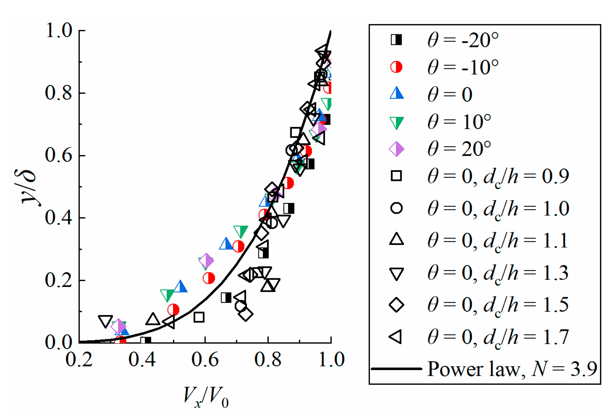
4.1. Vortex Formation and Velocity Distribution

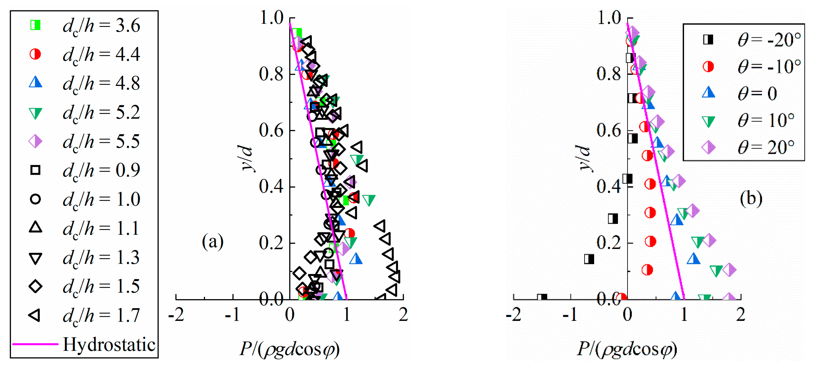
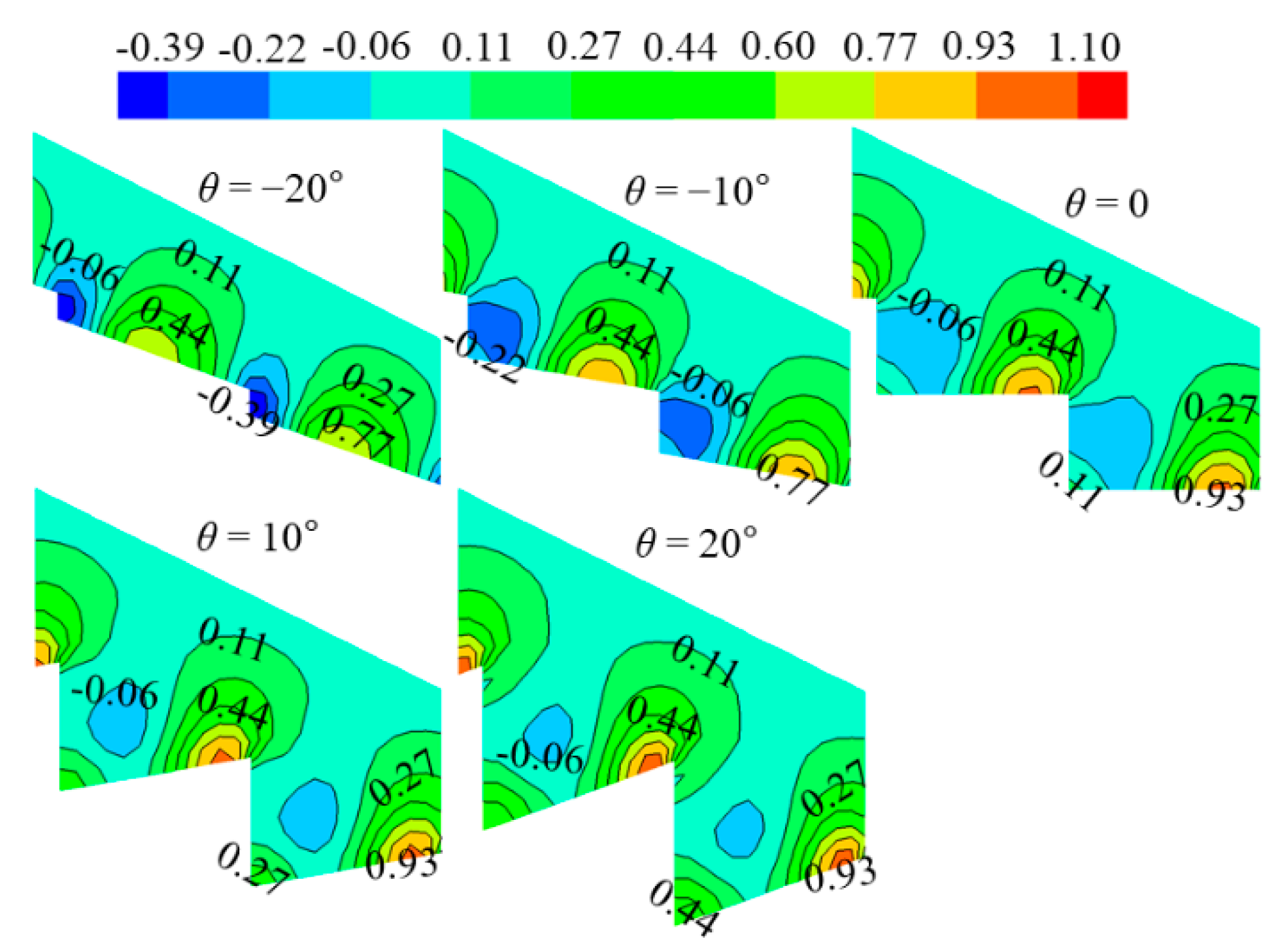
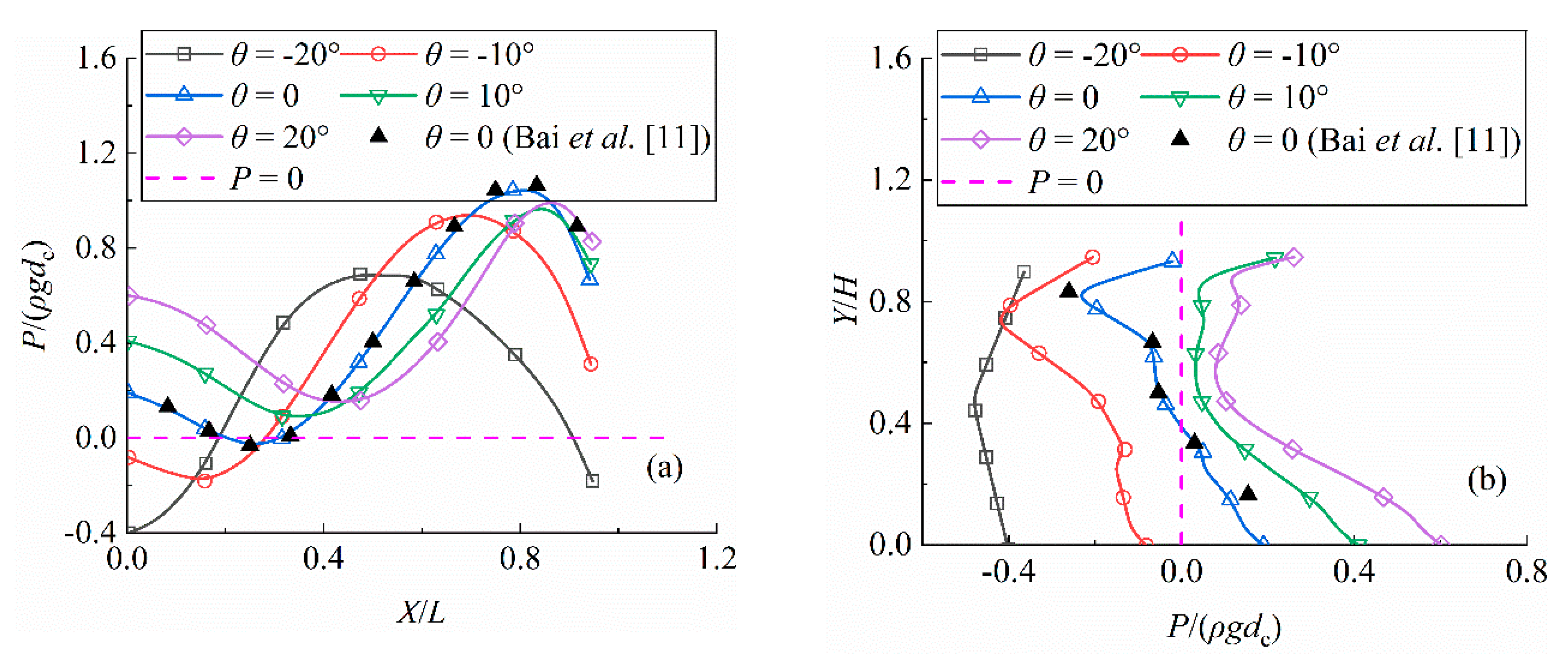
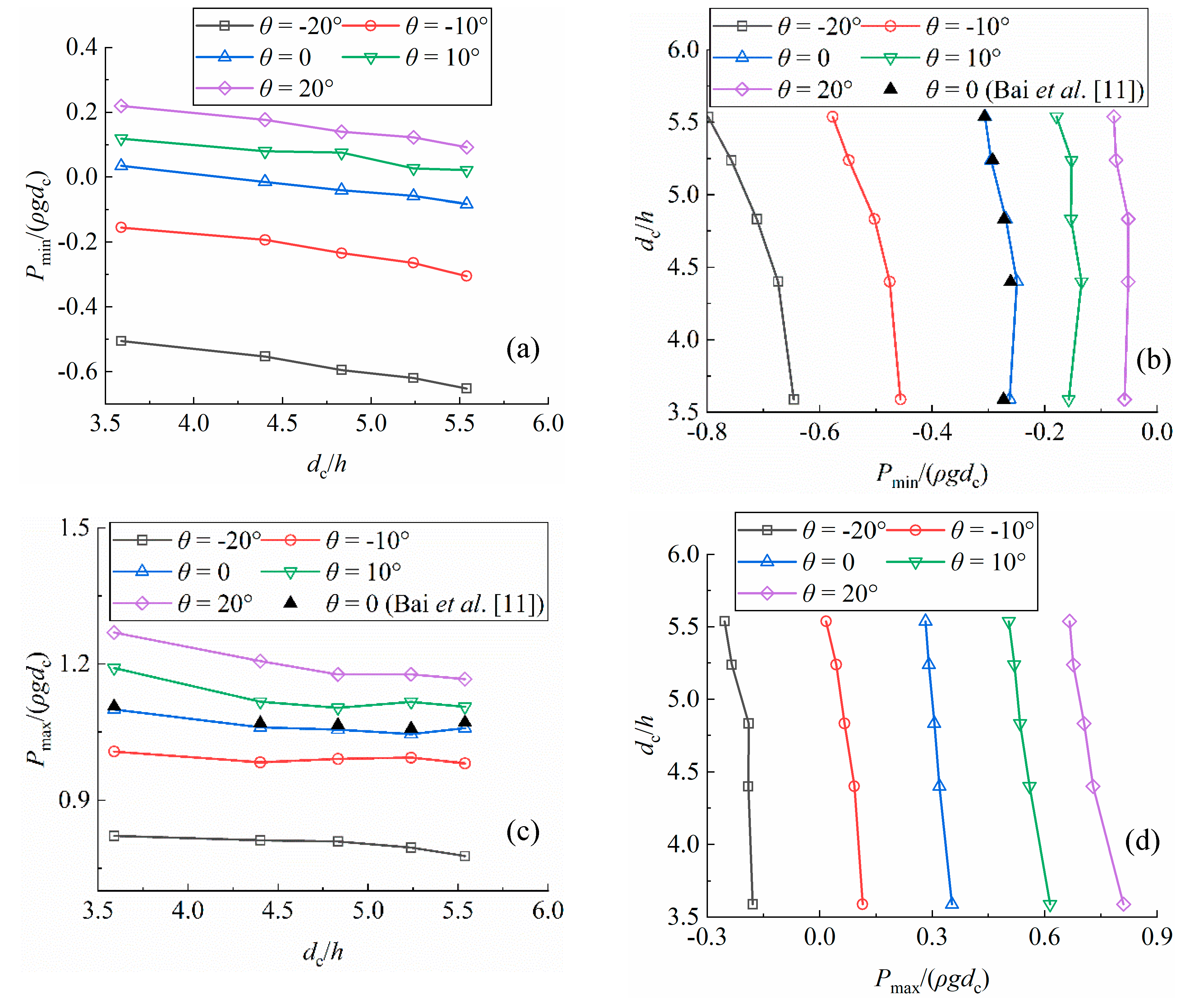
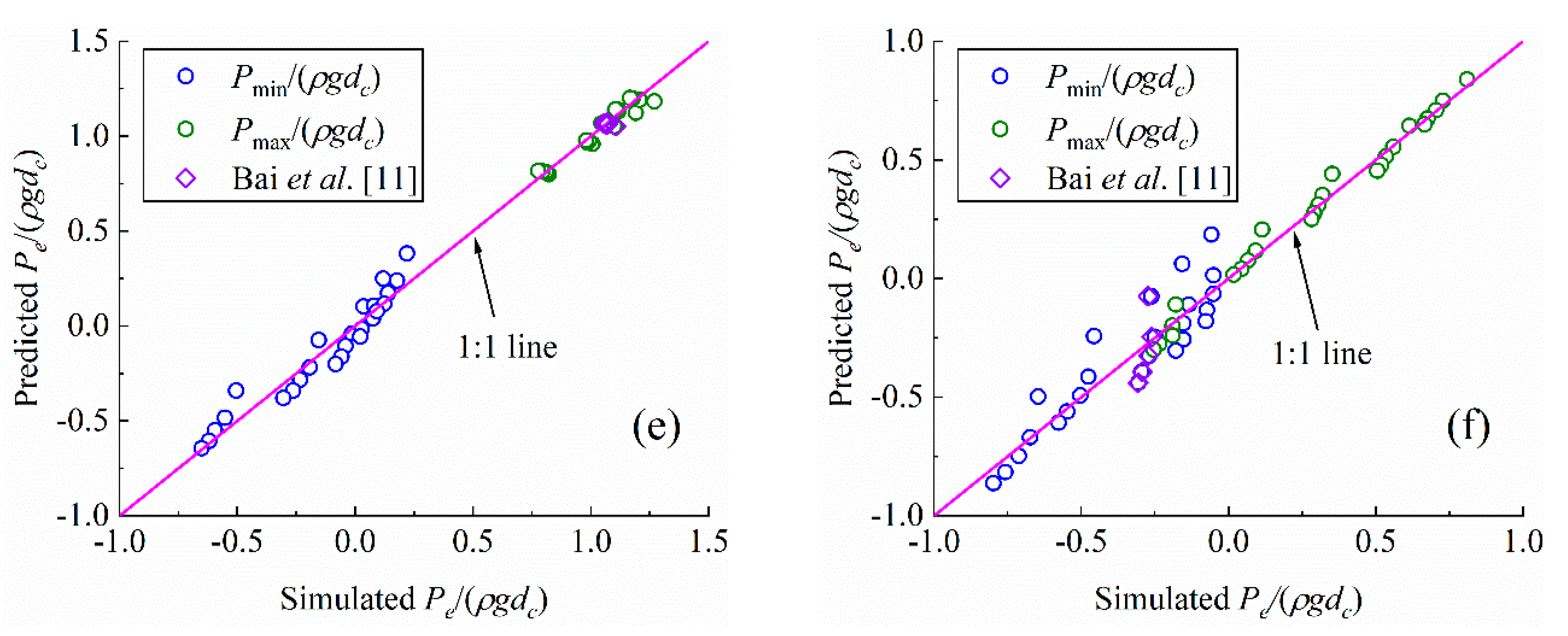
Along the symmetry plane, Figure 2a showcases, at d_c/h = 4.8, the flow fields at different θ values. The illustrated steps are no. 42 and 43. Over the steps, the flow exhibits a coherent structure with vortex formation in the step cavities. The flow patterns of the step layouts are similar. However, the vortex structures in the cavities differ in extent. The extent of the vortex flow becomes larger with an increase in θ. A larger vortex structure enhances the momentum exchange and energy dissipation. The vortices almost disappear if the step inclination gets larger downwards (e.g., θ = −20°), which is due to the fact that the roughness effects becomes smaller. The vortex characteristics affect the degree of energy loss of the flow [14]. To visualize the vortex structures, the Q-criterion, Q_c, is introduced

$$Q_c=\frac{1}{2}\left({\Vert {\mathsf{\Omega }}_{ij}\Vert }^2-{\Vert S_{ij}\Vert }^2\right)$$

(9)

in which

$${\mathsf{\Omega }}_{ij}=\frac{1}{2}\left(\frac{\partial u_i}{x_j}-\frac{\partial u_j}{x_i}\right)$$

(10)

$$S_{ij}=\frac{1}{2}\left(\frac{\partial u_i}{x_j}+\frac{\partial u_j}{x_i}\right)$$

(11)

Ω_ij = rate of rotation tensor, and S_ij = rate of strain tensor. They represent pure rotational motion and irrotational motion, respectively. In the fluid, if Q_c > 0, rotation is the dominant motion. If Q_c < 0, deformation is the main motion pattern. However, due to experimental error and viscous diffusion, Q_c = 0 cannot indicate the existence of vortex. Based on this method, the iso-surface of the vortex is identified in each layout, shown in Figure 2b (d_c/h = 4.8, Q_c = 100). The primary vortex characteristics are captured by Q-criterion. The vortex structures appear immediately downstream the vertical step faces. They cover an approximately cylindrical area in the step cavities and span across the channel width. There is a small region below the step vertices without vortex, which is possibly caused by the collision between the overlaying flow and up-climbing circulating flow. To compare the scale of the vortex, the area of its cross-section A is evaluated. Generally, A increases from downward to upward cases. For instance, compared with the conventional model, a 20° downward inclination leads to a 78% decrease, while a 20° upward inclination results in a 59% increase.

The flow over the steps features a developing boundary layer, above which there is an ideal flow region [23]. In this region down the spillway, the flow accelerates due to gravity and the velocity varies significantly. For the boundary layer, an analytical approach is used to predict the velocity distribution [24,25]. At a step’s vertex, the power law provides an approximation:

$$\frac{V_x}{V_0}={\left(\frac{y}{\delta }\right)}^{1/N}$$

(12)

where V_x = velocity component in the x-direction, V₀ = free stream velocity, δ = boundary layer thickness defined in terms of 0.99 V₀, and N = exponent. For all the θ and q values, the velocity profile of this study is best fitted with N = 3.9.

In the developing flow region, the numerical results are also compared with those by Zhang and Chanson [23], in which experiments were conducted for a stepped spillway sloping at 45° and with horizontal steps (θ = 0). Six flow discharges were examined. Figure 3 shows comparisons of the velocity distributions in a normalized form (V_x/V₀). The results in this study refer to d_c/h = 4.8 at the five θ values; the data from Zhang and Chanson [23] correspond to d_c/h = 0.9–1.7 at the same θ value (θ = 0). The latter is best fitted with N = 4.5. A similar distribution pattern is observed in the present research. Furthermore, at larger downward inclination (e.g., θ = −20°), the velocity gets larger for y/δ < 0.5, which is associated with the reduced bottom roughness. At y/δ > 0.5, the velocity difference is insignificant.

4.2. Flow Pressure

Due to the abrupt change in the channel bed, a stepped spillway features flow separations and significant pressure drop, which may give rise to cavitation damages. Caused by flow acceleration, the pressure fluctuates significantly in the developing flow region [23]. Along the y direction at the vertex of step no. 10, Figure 4a shows the pressure distributions, P/(ρgdcosφ), at θ = 0 and the different d_c/h values, where d denotes the water depth. For comparison, the results from Zhang and Chanson [23] are also included. Despite the difference in the step layouts, the numerical results exhibits the same trend as the experimental ones (open symbols), all with a larger ∂P/∂y gradient than the hydrostatic near the water surface. Figure 4b compares the effects of θ on the P/(ρgdcosφ) distribution. In the near-surface (ideal flow) region, the pressure distributions for all examined angles, except for θ = −20°, exhibit approximately a linear trend. The θ = −20° layout leads to the lowest P/(ρgdcosφ) values, which is attributable to the smallest step heights. The discrepancy from the hydrostatic distribution is presumably caused by the large velocity gradients. In addition, the flow pressure becomes higher with an increase in θ.

Along the symmetry plane, Figure 5 presents the pressure contours, P/(ρgd_c), at steps no. 42 and 43. The sudden change in the bed profile results in flow circulations and substantial pressure drop downstream of the vertical step face. Therefore, the pressures in the step cavities are low; the effects of θ on the low-pressure extents are also evident. If the downward inclination is significant (e.g., θ = −20°), negative pressure occurs on the entire vertical step face. For the downward angles, the low-pressure area in the step cavity becomes smaller if the inclination gets larger. For the upward angles, its size declines with an increase in θ. The dimensionless pressure, P/(ρgd_c), near the cavity corner becomes higher with an increasing θ. On the horizontal step surface, a high-pressure region is also observed, which is associated with the reattachment of the mainstream.

Along the step surfaces, both horizontal and vertical, Figure 6 compares the pressure distributions along the symmetry plane, in which Y = distance along a vertical step surface with its origin at the cavity corner. In the study made by Bai et al. [11], the θ = 0 layout is also numerically examined at d_c/h = 4.8, and their results are included in the diagram. Obviously, the differences in between are negligibly small. Along the horizontal steps, moderately inclining the steps, either downward or upward, exerts insignificant impacts on the pressure patterns. An S-shaped variation is seen with its max. values at X/L = 0.7–0.9, exclusive of the θ = −20° layout that has smallest steps close to the bottom. Along the vertical steps, the pressures in all cases demonstrate a descending trend, followed by an upward increase. The pressure gets larger as θ increases, with its min. occurring approximately at Y/H = 0.8 (except for θ = −20°).

On the step surfaces, the min. and max. pressures, denoted as P_min and P_max, provide insight into cavitation status and hydraulic loads. The extreme pressure P_e (or P_min and P_max) is associated with the flow condition (q), step geometry (h, l, and θ), flow property (ρ), and gravity (g). Therefore, these parameters are selected to describe P_e

$$P_e=f_1(q,h,l,\theta ,\rho ,g)$$

(13)

As d_c = (q²/g)^1/3 and θ is dependent on H, Equation (13) is expressed in a dimensionless form

$$\frac{P_e}{\rho g{d}_c}=f_2\left(\frac{d_c}{h},\frac{h}{l},\frac{H}{h}\right)$$

(14)

where h/l represents the channel slope and is a constant in a given spillway. Thus, P_e/(ρgd_c) is a function of d_c/h and H/h. Figure 7a–d present correlation of P_min and P_max with d_c/h under different θ. On the horizontal step surface (Figure 7a,c), both P_min and P_max become larger as the flow rate increases, which is consistent with the findings by Bai et al. [11]. The pressures at θ = −20° correspond to the lowest values. If implemented in a prototype, a large downward angle is more prone to cavitation, as its P_min is more likely to drop below the vapour pressure. The layout at θ = 20° exhibits the highest pressures. Ranging from θ = −20° to 20°, the P_max values differ on average by 49.4%. On the vertical step surface, the extreme pressures are compared in Figure 7b,d. For a fixed θ value, both P_min and P_max become higher if d_c/h gets smaller, which is in agreement with the results by Bai et al. [11]. Similar to the horizontal steps, to gradually change from a downward to upward angle contributes to an ascending P_min. However, an increase in θ also leads to an increase in the maximum pressure load. It is even noted that P_max at θ = −20° is negative, indicating that the entire vertical face is subjected to sub-pressure.

Based on the dimensional analysis from Equation (14), a correlation is proposed to estimate the extreme pressures on the horizontal and vertical step face

$$\frac{P_e}{\rho g{d}_c}=a\ln \left(\frac{d_c}{h}\right)+{\left(\frac{H}{h}\right)}^b$$

(15)

where a and b are coefficients. Their values are shown in

Table 3. Coefficients in Equation (15).

	Pmin		Pmax
	a	b	a	b
Horizontal face	−0.7016	0.4501	0.0410	0.2244
Vertical face	−0.8408	0.4225	−0.4377	0.6136

. For P_e on the horizontal step surface (Figure 7e), Equation (15) presents a satisfactory estimation, with the coefficient of determination R² > 0.91. The discrepancy of most data points is less than 10%. For P_e on the vertical step surface (Figure 7f), its prediction by Equation (15) shows a generally good agreement with the simulation (R² > 0.80).

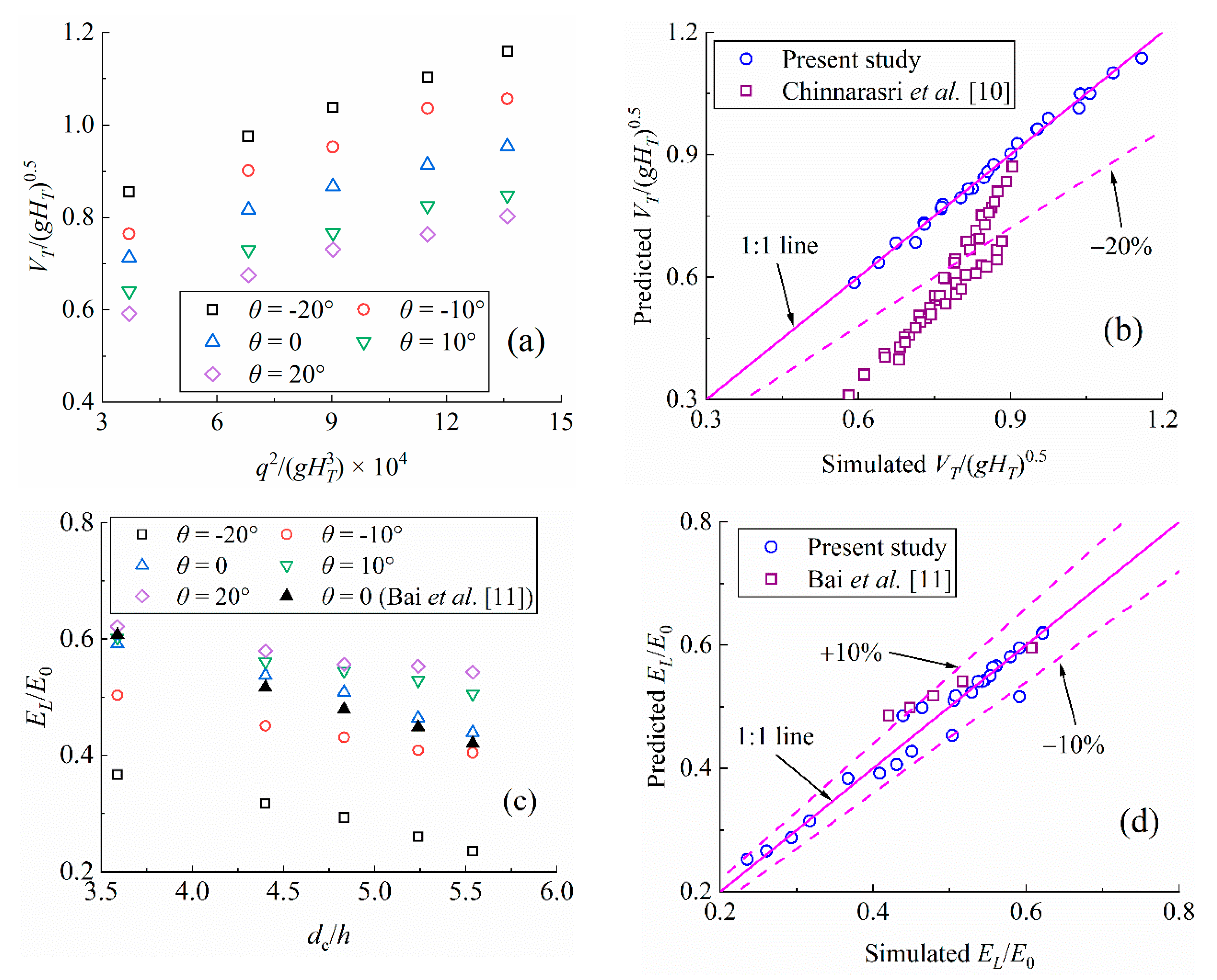
4.3. Energy Dissipation

Effective energy dissipation is essential for the protection of downstream riverbeds and structures. To estimate the residual energy downstream of the spillway, the averaged flow velocity at the chute end V_T is analyzed. V_T is an indicator of the energy dissipation. If more energy is dissipated by the steps, both the residual kinetic energy and V_T are smaller. V_T is dependent on H_T, q, h, l, θ, and g. It is expressed as

$$V_T=f_3\left(H_T,q,h,l,\theta ,g\right)$$

(16)

Based on Buckingham Pi theory, Equation (16) is rewritten in a dimensionless form as

$$\frac{V_T}{{\left(g{H}_T\right)}^{0.5}}=f_4\left(\frac{q^2}{g{H}_T^3},\frac{h}{l},\theta \right)$$

(17)

Define V_T/(gH_T)^0.5 = velocity ration, and $q^2/\left(g{H}_T^3\right)$ = drop number. For a given spillway chute, h/l represents its slope and is a constant. Therefore, the velocity ratio is a function of the drop number and inclination angle. Figure 8a illustrates the variation of V_T/(gH_T)^0.5 with $q^2/\left(g{H}_T^3\right)$ for different θ. The simulations indicate that at, for example, q = 0.31 m²/s, V_T ranges from 4.64 m/s at θ = −20° to 3.21 m/s at θ = 20°. Moreover, at a given θ value, the velocity ratio exhibits an almost linear upward trend with an increase in the drop number, showing that a larger discharge gives rise to higher residual energy. At a fixed drop number, the velocity ratio descends with an increase in θ. Shifting from θ = −20° to 20°, the velocity ratio drops on average by 44.0%. Compared to the upward layouts, the residual energy of the downward ones is larger.

Herein, based on Equation (17), an empirical equation is developed to estimate the velocity ratio. It is

$$\frac{V_T}{{\left(g{H}_T\right)}^{0.5}}={\lambda }_1\ln \left(\frac{q^2}{g{H}_T^3}\right)+{\lambda }_2\theta +{\lambda }_3$$

(18)

where λ₁, λ₂ and λ₃ are coefficients. Their values are listed in

Table 4. Coefficients in Equations (18), (20) and (21).

	λ1	λ2	λ3	α1	α2	β1	β2
θ ≤ 0	0.2136	−0.0087	2.3731	0.1745	1.2072	−0.3784	−0.2083
θ > 0	0.1602	−0.0049	1.9210	0.7519	1.8548	−0.5718	−0.2284

. In comparison with the experimental data on an upward inclined stepped chute [10], Figure 8b shows the predicted velocity ratios against the simulated ones. Equation (18) gives an acceptable estimation of the velocity ratio, with R² > 0.98. Nevertheless, it generally overestimates the physical results, which is likely associated with the difference in the chute slope.

The relative energy loss, defined as E_L/E₀, is another parameter to quantify the energy dissipation of a stepped spillway, in which E_L = energy loss between two cross-sections and E₀ = total energy head at the upper cross-section. Together with the θ = 0° results by Bai et al. [11], Figure 8c shows the variation of E_L/E₀ with d_c/h. The agreement is generally good. Similar to the findings by Chen et al. [26], Zare and Doering [27] and Felder and Chanson [28], E_L/E₀ exhibits a downward trend with an increasing d_c/h. For the θ = −20° chute, E_L/E₀ is much smaller than for the other layouts, which is ascribed to the smaller bottom friction elements. Under the same flow conditions, a progressive transition from a down- to upward step surface enhances the roughness effect and boosts the energy dissipation. This is because the inclined steps obstruct the flow, producing more spray and trapping recirculation vortices in the step cavities. Compared with θ = 0°, the θ = 20° layout results, for example, in 6.3% more energy dissipation, while the θ = −20° layout leads to about 21.3% less dissipation.

As shown in Figure 8c, all data follow a similar tendency. E_L/E₀ is proportional to d_c/h, and a correlation is presented to desirable their relationship.

$$\frac{E_L}{E_0}=\eta {\left(\frac{d_c}{h}\right)}^{\zeta }$$

(19)

where η and ζ = coefficients. Based on the simulated results, they are determined by

$$\eta ={\alpha }_1\ln \left(\frac{h}{l}·\frac{h}{H}\right)+{\alpha }_2$$

(20)

$$\zeta ={\beta }_1\ln \left(\frac{l}{H}\right)+{\beta }_2$$

(21)

where α₁, α₂, β₁ and β₂ are coefficients. Their values are shown in Table 4. Figure 8d compares the simulated E_L/E₀ values with the predicted ones. Equation (19) gives a reasonable estimation of the calculated E_L/E₀, as well as the reference data [11]. Most data fall within the ±10% error limit. The average and max. discrepancy is 3.3% and 12.7%, respectively.

5. Conclusions

A stepped spillway is a flood release structure with effective aeration and energy dissipation. Along with the rapid construction of roller-compacted concrete (RCC) dams, many such spillways have been built. Conventionally, the stepped chute features horizontal step surfaces. Due to large dam heights, the cavitation risk associated with local low pressure is often an issue of concern in design. Revised flood criteria might require that a dam spillway should safely discharge extreme floods higher than the original design flood.

With an aim to overcome the shortcomings of the conventional layout, a few step arrangements are devised with modifications in the step angling. CFD modelling is performed to evaluate how they affect the flow behaviors. The results are analyzed to look into flow velocity, pressure, cavitation potential and level of energy dissipation. The major conclusions are as follows:

• In the step cavities, the extent of flow circulations becomes larger with an increase in inclination angle. At a step vertex in the developing flow region, the power law gives a good description of the flow velocity above the pseudo-bottom, exhibiting an inverse correlation with the inclination angle.
• Along the horizontal step surface, the flow pressures exhibits an S-shaped change, except for at the 20° downward inclination. The min. and max. pressures become lower at a larger flow discharge and higher at a smaller inclination angle. A high-pressure zone is observed on the step surface, with a smaller pressure magnitude in the downward layouts than in the upward ones. A correlation is suggested to estimate the extreme pressures.
• Along the vertical step surface, the water pressure declines from the bottom, followed by a slight increase. The entire vertical face is subjected to negative pressure if the downward step angle is large (i.e., −20°). Both the min. and max. pressure demonstrates a descending trend with an increase in flow discharge. In the small-angle layouts, the extreme pressures are lower than in the large-angle ones.
• An increase in the drop number leads to an increase in the velocity ratio at the chute end. With an increase in flow discharge at a given step angle, the energy dissipation becomes less effective (lower energy loss). A gradual change from a downward to an upward step results in more energy loss. In comparison with the conventional layout, the 20° upward inclination dissipates 6.3% more energy, while a 20° downward angle dissipates 21.3% less energy. Empirical equations are presented to predict the velocity and energy dissipation.

This study shows that it is feasible to improve the hydraulic behaviors of a stepped chute if the horizontal step angling is modified. A layout with a moderately upward step (e.g., 10°) is recommended if energy dissipation is a major issue of concern. For example, compared with the horizontal steps, the 10° upward step reduces the end velocity by 10.7% and enhances on average the energy dissipation by 8.0%. Meanwhile, the lowest pressures on both the horizontal and vertical step surfaces are improved, which mitigates the cavitation risk in a prototype. Because of its less effective energy dissipation and low-pressure on the whole vertical surface, the downward steps are not advisable to use.

References

1. Chanson, H. Hydraulics of stepped spillways: Current status. J. Hydraul. Eng. 2000, 126, 636–637. [Google Scholar] [CrossRef]
2. Peyras, L.; Royet, P.; Degoutte, G. Flow and energy dissipation over stepped gabion weirs. J. Hydraul. Eng. 1992, 118, 707–717. [Google Scholar] [CrossRef]
3. Boes, R.M.; Hager, W.H. Hydraulic design of stepped spillways. J. Hydraul. Eng. 2003, 129, 671–679. [Google Scholar] [CrossRef] [Green Version]
4. Guenther, P.; Felder, S.; Chanson, H. Flow aeration, cavity processes and energy dissipation on flat and pooled stepped spillways for embankments. Environ. Fluid Mech. 2013, 13, 503–525. [Google Scholar] [CrossRef] [Green Version]
5. Zhang, G.; Chanson, H. Air-water flow properties in stepped chutes with modified step and cavity geometries. Int. J. Multiphas. Flow 2018, 99, 423–436. [Google Scholar] [CrossRef] [Green Version]
6. Ghaderi, A.; Abbasi, S.; Abraham, J.; Azamathulla, H.M. Efficiency of trapezoidal labyrinth shaped stepped spillways. Flow Meas. Instrum. 2020, 72, 101711. [Google Scholar] [CrossRef]
7. Wüthrich, D.; Chanson, H. Hydraulics, air entrainment, and energy dissipation on a Gabion stepped weir. J. Hydraul. Eng. 2014, 140, 04014046. [Google Scholar] [CrossRef]
8. Felder, S.; Chanson, H. Effects of step pool porosity upon flow aeration and energy dissipation on pooled stepped spillways. J. Hydraul. Eng. 2014, 140, 04014002. [Google Scholar] [CrossRef] [Green Version]
9. Gonzalez, C.; Chanson, H. Turbulence and cavity recirculation in air–water skimming flows. J. Hydraul. Res. 2008, 46, 65–72. [Google Scholar] [CrossRef]
10. Chinnarasri, C.; Wongwises, S. Flow regimes and energy loss on chutes with upward inclined steps. Can. J. Civ. Eng. 2004, 31, 870–879. [Google Scholar] [CrossRef]
11. Bai, Z.; Wang, Y.; Zhang, J. Pressure distributions of stepped spillways with different horizontal face angles. Ice-Water Manag. 2017, 171, 299–310. [Google Scholar] [CrossRef]
12. Bayon, A.; Toro, J.P.; Bombardelli, F.A.; Matos, J.; López-Jiménez, P.A. Influence of VOF technique, turbulence model and discretization scheme on the numerical simulation of the non-aerated, skimming flow in stepped spillways. J. Hydro-Environ. Res. 2018, 19, 137–149. [Google Scholar] [CrossRef] [Green Version]
13. Bai, Z.; Peng, Y.; Zhang, J. Three-dimensional turbulence simulation of flow in a V-shaped stepped spillway. J. Hydraul. Eng. 2017, 143, 06017011. [Google Scholar] [CrossRef]
14. Chen, Q.; Dai, G.; Liu, H. Volume of fluid model for turbulence numerical simulation of stepped spillway overflow. J. Hydraul. Eng. 2002, 128, 683–688. [Google Scholar] [CrossRef]
15. Longo, S.; Di Federico, V.; Archetti, R.; Chiapponi, L.; Ciriello, V.; Ungarish, M. On the axisymmetric spreading of non-Newtonian power-law gravity currents of time-dependent volume: An experimental and theoretical investigation focused on the inference of rheological parameters. J. Non Newton. Fluid 2013, 20, 69–79. [Google Scholar] [CrossRef]
16. Di Federico, V.; Longo, S.; King, S.E.; Chiapponi, L.; Petrolo, D.; Ciriello, V. Gravity-driven flow of Herschel–Bulkley fluid in a fracture and in a 2D porous medium. J. Fluid Mech. 2017, 821, 59–84. [Google Scholar] [CrossRef] [Green Version]
17. Shi, Q.S. High-Velocity Aerated Flow, 1st ed.; Water & Power Press: Beijing, China, 2007; pp. 68–75. (In Chinese) [Google Scholar]
18. Celik, I.B.; Ghia, U.; Roache, P.J.; Freitas, C.J. Procedure for estimation and reporting of uncertainty due to discretization in CFD applications. J. Fluid Eng. Trans. ASME 2008, 130, 078001. [Google Scholar]
19. Boes, R.M.; Hager, W.H. Two-phase flow characteristics of stepped spillways. J. Hydraul. Eng. 2003, 129, 661–670. [Google Scholar] [CrossRef]
20. Chanson, H. Air-water flow measurements with intrusive, phase-detection probes: Can we improve their interpretation? J. Hydraul. Eng. 2002, 128, 252–255. [Google Scholar] [CrossRef] [Green Version]
21. Chanson, H. Hydraulics of skimming flows over stepped channels and spillways. J. Hydraul. Res. 1994, 32, 445–460. [Google Scholar] [CrossRef] [Green Version]
22. Rajaratnam, N. Skimming flow in stepped spillways. J. Hydraul. Eng. 1990, 116, 587–591. [Google Scholar] [CrossRef]
23. Zhang, G.F.; Chanson, H. Hydraulics of the developing flow region of stepped spillways. II: Pressure and velocity fields. J. Hydraul. Eng. 2016, 142, 04016016. [Google Scholar] [CrossRef] [Green Version]
24. Chanson, H. The Hydraulics of Open Channel Flow: An Introduction, 1st ed.; Edward Arnold: London, UK, 1999; pp. 66–71. [Google Scholar]
25. Chanson, H. The Hydraulics of Stepped Chutes and Spillways, 1st ed.; Balkema: Lisse, The Netherlands, 2001; pp. 210–213. [Google Scholar]
26. Chen, Q.; Dai, G.; Zhu, F. Influencing factors for the energy dissipation ratio of stepped spillways. J. Hydrodyn. 2005, 17, 50–57. [Google Scholar]
27. Zare, H.K.; Doering, J.C. Energy dissipation and flow characteristics of baffles and sills on stepped spillways. J. Hydraul. Res. 2012, 50, 192–199. [Google Scholar] [CrossRef]
28. Felder, S.; Chanson, H. Aeration, flow instabilities, and residual energy on pooled stepped spillways of embankment dams. J. Irrig. Drain. Eng. 2013, 139, 880–887. [Google Scholar] [CrossRef] [Green Version]
Figure 1. Sketch of the spillway (a) stepped spillway, (b) conventional layout θ = 0, (c) upward step θ > 0, and (d) downward step θ < 0.
Applsci 10 06202 g001
Figure 2. Flow fields at the steps at different θ values (for dc/h = 4.8 at steps no. 42 and 43): (a) velocity vectors, and (b) vortex structures (Qc = 100).
Applsci 10 06202 g002
Figure 3. Velocity distributions in the boundary layer at vertices of step no. 10. A half-filled symbol refers to numerical results (this study), and an open one to experimental ones [23].
Applsci 10 06202 g003
Figure 4. Pressure distributions at the step vertex (step no. 10): (a) θ = 0, and (b) dc/h = 4.8. A half-filled symbol refers to numerical results of this study, and an open one to experimental ones by Zhang and Chanson [23].
Applsci 10 06202 g004
Figure 5. Pressure contours (P/ρgdc) at different θ values at steps no. 42 and 43 (dc/h = 4.8).
Applsci 10 06202 g005
Figure 6. Flow pressure distribution along step surfaces at step no. 43 (dc/h = 4.8): (a) horizontal and (b) vertical.
Applsci 10 06202 g006
Figure 7. Extreme pressures acting on step surfaces at step no. 43: (a,c,e) horizontal face, and (b,d,f) vertical face.
Applsci 10 06202 g007aApplsci 10 06202 g007b
Figure 8. Energy dissipation characteristics: (a) Velocity ratio, (b) simulated against predicted velocity ratio, (c) relative energy loss and (d) simulated against predicted energy loss.
Applsci 10 06202 g008