GIS Spatial Optimization for Corridor Alignment Using Simulated Annealing

Featured Application

This research allows tracing optimized routes in corridors of long lengths and is applied to the installation of pipelines that transport valuable liquids, which can be oil or petroleum.

Abstract

Planning corridors for new facilities such as pipeline or transmission lines through geographical spaces is a topographical constraint optimization problem. The corridor planning problem requires finding an optimal route or a set of alternative paths between two locations. This article presents a simulated-annealing-based (SA) approach applying a variable neighborhood strategy in a continuous space to generate competitive and different alternative paths to solve the corridor planning problem. The variable neighborhood method randomly selects two points from a variable interval of the current solution generated by SA creating pseudo-random paths inside a corridor and finding spatially different alternatives. The proposed approach is evaluated with three practical problems using real topographic data from the Veracruz Basin in Mexico. The experimental results show that this approach obtains efficient and competitive solutions with improvements above 18% over those gotten by the compared method.

1. Introduction

Corridor is an indispensable requirement to build linear installations such as pipelines, electric transmission lines, communications ways, etc. [1,2]. The corridor planning process must consider legal, social, political, environmental, and economic factors interfering and making the corridor design complex [3]. However, proper corridor planning involves identifying alternative routes and selecting the best one based on design specifications, environmental laws, and good practices [4]. The corridor planning problem is generally addressed by one or more selection criteria such as distance, environmental impact, and safety, and it is modeled as an optimization problem subject to several topographical constraints [2,5].

According to [6], locating an optimal corridor is analogous to identifying the shortest or least expensive path between two points. Traditional approaches generate a set of alternative routes using enumerative methods with penalty techniques or by specifying one or multiple intermediate points where the path must pass [7,8,9]. The running time of these methods tends to grow exponentially, depending on the size of the geographical study area. In addition, the generation of near-optimal alternative routes in reasonable times using exact methods is hard since they find only one solution in their searching process [10].

Nowadays, the creation of new corridors to provide different services through linear facilities is growing for the emergence and expansion of urban areas. However, their construction can be delayed due to poor planning, so generating alternative routes for evaluating and comparing candidate solutions is crucial in the corridor planning process. The problem of making alternative routes has led researchers to develop diverse solution methods using different problem representations and applying several deterministic shortest-path-search algorithms such as the Dijkstra algorithm [11] and its variants. However, generating alternative routes requires exploring the geographical study area, and exact methods only get one route at a time. Thus, an efficient method must include mechanisms allowing the examination of alternative routes spatially dispersed, in reasonable computing time. On the other hand, non-deterministic approaches such as swarm and evolutionary algorithms, and the simulated annealing can find near-optimal solutions in a reasonable time due to their exploration and exploitation skills.

This paper presents a simulated-annealing-based optimization method applying a variable-neighborhood structure to generate and evaluate alternative corridor routes and select the best one. The proposed algorithm starts its search process with a feasible solution obtained by a greedy uninformed search strategy, the breadth-first-search (BFS) algorithm, which does not use some cost function for exploring possible routes, and not necessarily find the optimal global path. Then, the variable neighborhood mechanism randomly selects two points in the corridor for exploring alternative routes through prohibited and guided movements. The results obtained with the simulated annealing method are compared with the BFS algorithm, to show the effectiveness in improving the solutions obtained by the proposed algorithm. The experimental analysis compares the variable-neighborhood mechanism on three real problem scenarios. It suggests that the proposed mechanism explores and improves the initial solution. Likewise, the neighborhood structure permits creating and evaluating alternative corridor routes and selecting the best one, based on the objective value. Improvements are reported above 18% on the greedy algorithm in the solution quality.

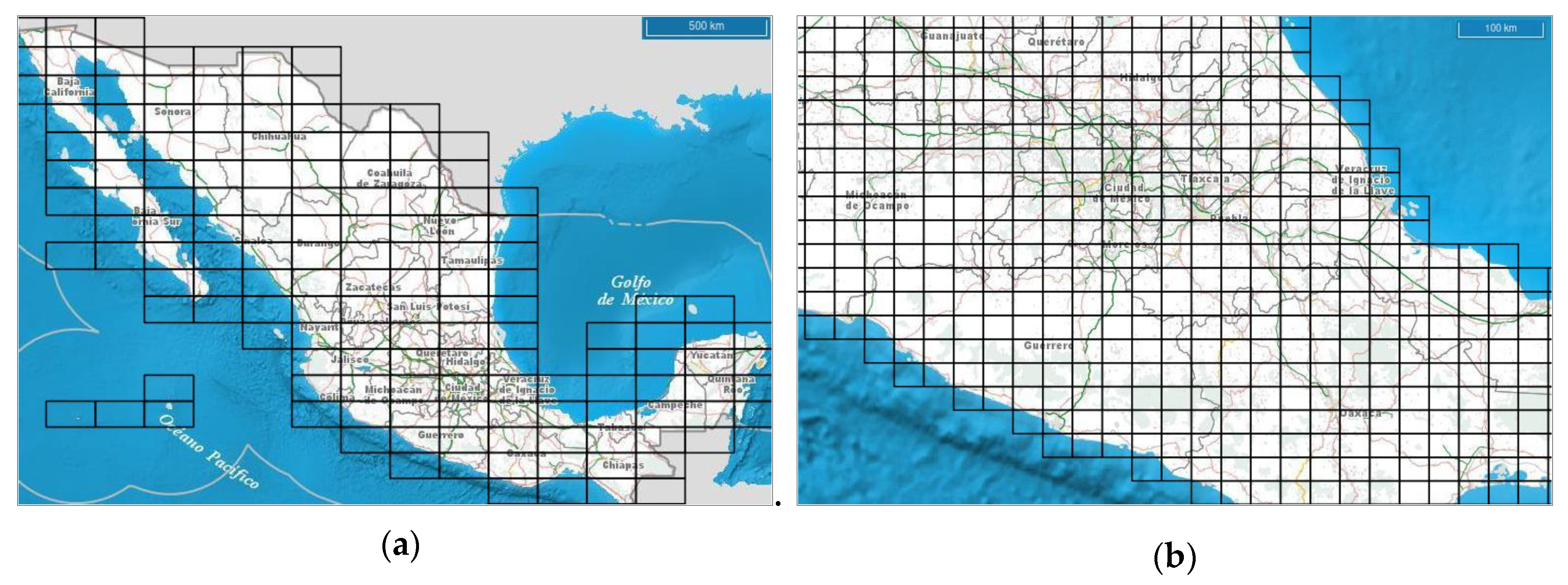
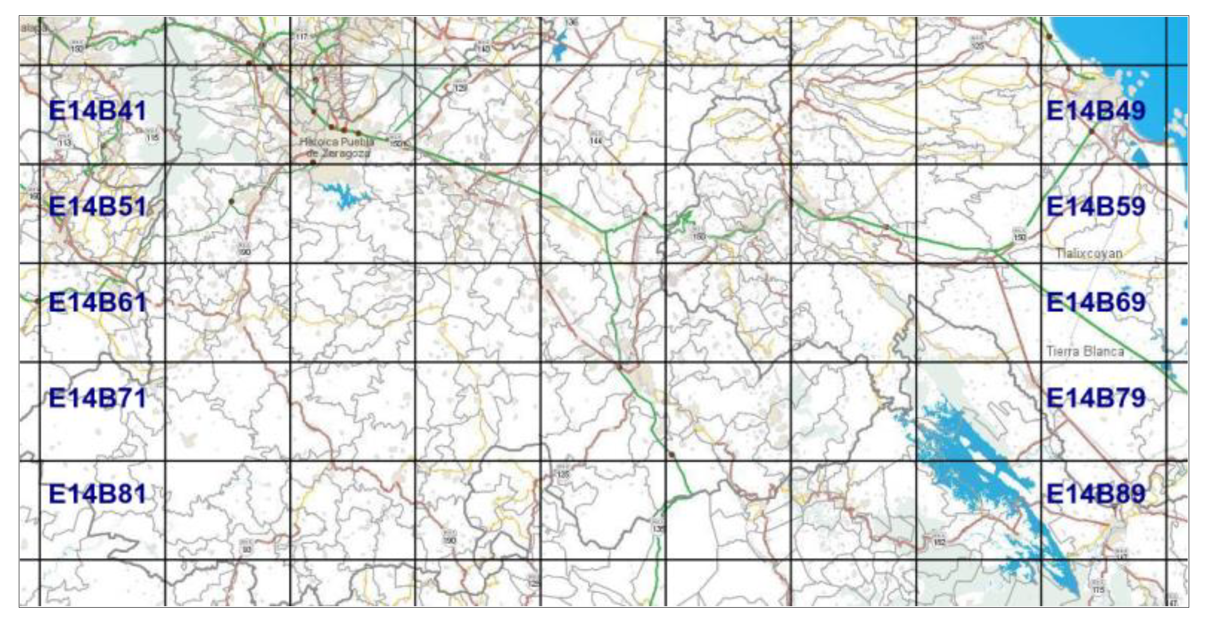
The main contribution of this work is the implementation of a variable-search mechanism generating alternative routes inside a corridor. The proposed algorithm dynamically selects the best route considering topographic information collected from three Mexican regions located in the Veracruz Basin. It is a prominent oil and gas extraction area of excellent quality where several production fields are currently located.

The rest of the document is structured as follows: Section 2 describes the corridor planning problem and the optimization model of the shortest route. Section 3 depicts the simulated annealing algorithm elements: The initial solution creation procedure and the details of the variable-neighborhood structure. Section 4 provides details of the test scenarios, and the experimental results obtained with the SA algorithm. Finally, Section 5 shows the conclusions and future work.

2. Problem Statement

This section describes the corridor planning problem in general, and the related works proposed to address this problem. Finally, the optimization model used to find the shortest path on which this work is based is shown as well.

2.1. Problem Description

Research in the construction of linear facilities such as pipelines, transmission lines, and communication routes is essential to define the land corridor where they will be placed. A corridor is a geographic area between two points joined using several intermediate points, providing the necessary space for guaranteeing the right conditions for the construction and use of the facilities. In particular, the corridor-width depends on local regulations, according to the installation type. The corridor planning problem can be modeled as an optimization problem subject to topographical constraints [1,5,12]. Corridors are usually addressed by one or more selection criteria such as distance, environmental impact, safety, etc. The design of a topographical network representing the study region is part of the corridor planning process. Once this network is defined, a corridor between two points is selected from all possible paths.

The corridor planning process considers numerous factors affecting the project proposal [3,12]. In general, an initial corridor route is first determined and then refined using the design criteria [13]. In the first phase, the parties involved in the project must approve the proposed route according to the input data used in the spatial analysis [14]. This route can be modeled using a geographic information system (GIS) to assign the impact costs in the study area. GIS provides several algorithms to find the shortest path, but what is required in this work is to find multiple optimized routes within a corridor near the shortest route which is the global optimum. Therefore, a route refinement is necessary, where other competitive and near-optimal but spatially different solutions are considered [14]. The shortest path can be obtained by penalizing the distance of each step taken when crossing the region. However, a real problem may have obstacles complicating the movements in certain directions. Therefore, it is crucial to exploit the knowledge of the study region through spatial exploration and analysis [15], to classify the factors being part of the route selection criteria. Some of them are the ground elevation, soil type, vegetation type, and the presence of water bodies, roads, and archaeological zones. Other factors that should be considered are those disturbing humans and wild animals. Once the constraints have been defined using these factors, a feasible route can be found.

2.2. Existing Methodologies to Generate Alternate Routes

Several techniques to evaluate the number of alternate routes and solve the corridor planning problem have been described in the existing literature. The iterative penalty method [7] assigns penalty parameters to graph arcs once they are selected to be part of a candidate solution. This method is initially proposed for road design, but it has also been used for routing hazardous materials [16], among other applications. In [8], the gateway shortest path (GSP) method based on a constrained shortest path problem is introduced. The Global Positioning System (GPS) generates the shortest route between two points without passing through points known as gateways. GPS allows the identification of different acceptable alternative paths with less computational effort concerning penalty methods. The k-shortest-path algorithm [17] and the near-shortest path method [18] are two methods generating a set of lower-cost paths based on small variations of their initial solution.

Furthermore, the k-differentiated-path (kDP) algorithm proposed in [19] uses a minimax approach to find k-differentiated-shortest paths that are relatively different from one another, but not necessarily disjoint. On the other hand, the p-dispersion algorithm in [20] first creates a broad set of candidate routes, and then it selects a subset of them using a dispersion model, maximizing the minimum difference between any pair of selected routes. In [21], the authors locate corridors as a collection of adjacent polygons based on a quantitative criterion measuring the corridor length. This method selects one corridor to cross the polygons using the Dijkstra algorithm. In contrast, in [9], the authors use multiple gateways to generate more complex paths. This approach is similar to the GPS method, except for allowing that the route uses more than one gateway. Other proposed strategies use parallel computing to run their procedures, such as the kth-shortest path and the near-shortest path method [22,23]. The main disadvantage of these methods is that the needed time to reach an optimal solution grows exponentially as the problem size increases [24].

An alternative to deal with these problems is applying some non-deterministic heuristic capable of generating near-optimal solutions in a reasonable computation time. In [25,26,27,28,29], the authors use genetic algorithms (GAs) to optimize two and three-dimensional highway alignments. These approaches only differ in the objective function elements, such as right-of-way cost, travel-time cost, earthwork cost, structure cost, and socioeconomic cost. This formulation is also used by [30,31] to solve the rail transit alignment problem. In [32], a parallel GA to solve the intercity railway alignment problem is used. In [6], a multi-objective GA, named MOGADOR, for solving the general corridor alignment problem is applied, and the authors in [33,34] also use a multi-objective GA to solve the highway alignment problem. On the other hand, scarce application of other heuristics for the corridor planning problem has been described in the existing literature, such as the tabu search for alignment of forest roads [35] and simulated annealing [36], particle swarm optimization [37], and ant colony optimization [38] for the highway alignment problem.

2.3. Mathematical Model

The corridor planning problem is concerning finding the shortest path joining two specific nodes in an undirected weighted graph [6]. The mathematical model of the corridor routes is described by relations (1)–(5). The topographical network (rectangular mesh or grid) representing the study area is encoded using a graph (N, A), where N = {u₁, …, u_n} is the set of n nodes, and A = {(u₁, v₁), …, (u_m, v_m)} is the set of m edges connecting the nodes. A node represents the center of a cell in the rectangular mesh (matrix of visited nodes), and each edge is associated with a viability cost (penalty) $c_{u,v}^p\in R$ of passing from node u to node v in the graph. Furthermore, each edge has associated an elevation value $c_{u,v}^{DEM}$, based on a digital elevation model (DEM). In this model, s and t are the source and destination nodes connected by the corridor, respectively, and a binary variable $x_{uv}$ is used to indicate if the edge (u,v) is or not part of the route.

$$minz\left(x\right)=min{\displaystyle \sum }_{\left(u,v\right)\in A}{x}_{u,v}\left({\displaystyle \sum }_{l=1}^{l=Nl}p{l}_{u,v}+c_{u,v}^{DEM}\right),u\ne v$$

(1)

s.t.

$${\displaystyle \sum }_{\left(u,v\right)\in A}{x}_{uv}-{\displaystyle \sum }_{\left(v,u\right)\in A}{x}_{vu}=\{\begin{array}{cc}1& ifu=s\\ -1& ifu=t\\ 0& ifu\ne s,t\end{array}$$

(2)

$$x_{u,v}=\left\{0,1\right\},\forall \left(u,v\right)\in A$$

(3)

$$\left(u,v\right)\in corridor,\forall \left(u,v\right)\in A$$

(4)

$$c_{u,v}^{DEM}\le e_{max}$$

(5)

The goal, shown in Equation (1), is to find the lowest cost route from s to t, accomplishing the constraints expressed in (2)–(5). In this work, the route cost is a combination of the viability costs of the edges (u,v) belonging to the proposed route and the elevation of the visited nodes in the corridor. The route between nodes s = 0 and t = k is a finite sequence of nodes n = {u₀, ⋯, u_k}. The accumulated costs matrix represents the feasibility of passing between two nodes, using a feasibility scale of 1 to 10, where 1 represents the lowest penalty cost, i.e., there exists a priority to pass on the path, while value 10 means that it is prohibited. For creating this matrix, a feasibility cost p (penalty) for each topographic l (layer) is assigned according to its relevance. The values of the Nl layers involved in the corridor design are added and weighted in Equation (1). Equation (6) shows the weighting operation of a raster cell $c_{uv}^p$ in the accumulated cost matrix. Elevation on the ground is also penalized with higher values of $c_{uv}^{DEM}$ in Equation (1). Constraints (2) guarantees that s and t are only used as the initial and final node in the route, respectively, as well as no cycles are in the solution, fulfilling the constraints (3). Furthermore, constraints (4) indicates that edge (u, v) must be located within the corridor. The corridor is given in units of length and has as its midpoint the shortest route found by an exact algorithm such as the Dijkstra algorithm. Finally, constraint (5) establishes that e_max is the maximum elevation allowed on the ground.

$$c_{u,v}^p={{\displaystyle \sum }}_{l=1}^{l=Nl}p{l}_{u,v}$$

(6)

The optimization model presented in (1) to (5) is used to find cost-optimized routes located in the corridor generated by the shortest route. These optimized routes are obtained by the simulated annealing algorithm, which creates neighboring routes to the shortest route.

3. Simulated Annealing Approach for the Corridor Planning Problem

The shortest and least expensive routes between two geographical locations can be obtained applying exact methods, and a GIS facilitates their computation, as well as the spatial analysis and the management of geographic information by using robust data models [39,40,41]. Since a GIS commonly uses Dijkstra-based algorithms, the corridor width is not considered in their calculations, and alternative routes to the best one cannot be obtained [42]. The corridor width can be conceptualized in different ways based on the map scale, but one additional mechanism is needed to generate more than one route. In this case, heuristics are applied to reach near-optimal solutions in a reasonable time, since they are reliable and straightforward strategies for solving complex problems.

The simulated annealing (SA) algorithm is a heuristic technique finding near-optimal solutions for combinatorial problems with large solution spaces [43]. SA is based on a thermal treatment for solids, named annealing, where one material is exposed to high temperatures to the melting point and is cooled gradually to a cooling point. Annealing allows the molecules to organize themselves to reach minimal potential energy, thereby achieving higher resistance. The SA algorithm is used to solve complex optimization problems such as the traveling salesman problem [44], the automatic design of integrated circuits, and the noise suppression in digital images [45], as well as in image compression [46], among other problems. SA implements an iterative local search guided through a stochastic process with a given probability [47]. First, SA starts with an initial candidate solution s, and a high-temperature T. With an iterative structure, SA disturbs s until T reaches a value less than the stop criterion. During this process, in each iteration, a new candidate solution s’ is selected from the neighborhood of the current solution. These solutions are compared, and the best one is chosen as the new current solution. In some cases, a not improved solution is accepted to escape a local optimum and to continue searching for better solutions. 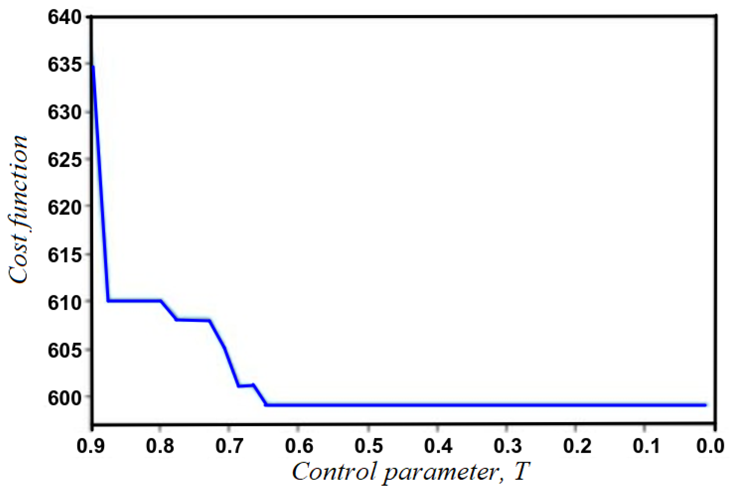The probability of taking not improved solutions depends on the T parameter, which decreases in each algorithm iteration using a control coefficient β. Since T starts with a high value, random changes are allowed. However, as the temperature is lowered slowly, the number of accepted changes decreases until the procedure reaches a stationary state. SA adopts different stochastic methods to determine the acceptance probability of a new solution but commonly uses the algorithm proposed by [48], where the energy change in a cooling process of a physical system is simulated. Thermodynamics laws state that at a temperature T, the probability of energy rise of magnitude ∆E is determined by the expression P(∆E) = e^−∆E/kT, where k is the Boltzmann constant.

It is clear that when SA perturbs only one solution in each stage of its iterative process, it promotes the solution space exploitation. Furthermore, by the use of its acceptance criteria, the solution space exploration is encouraged. Although other heuristics, such as swarm and evolutionary algorithms, have demonstrated to reach near-optimal solutions for diverse optimization problems, they consume more computational resources than that used by SA. These algorithms disturb a set of candidate solutions in each step of their iterative process, and this implies the evaluation of several solutions, unlike SA, evaluating only one candidate solution.

The SA algorithm applied in this paper to locate corridors explores alternative routes between the origin and destination node on each iteration, until the best one is found. The objective function considers both the minimum distance and the feasibility costs of passing on the study region. For improving the search procedure, diverse neighborhood structures are used, allowing found approximate solutions, adjusted to the complexity and nature of the problem [49]. Algorithm 1, shows the procedure to locate a near-optimal corridor. In this algorithm, s_i is the initial solution, m is the counter increasing until reaching the Markov chain length (L_markov) defining the Metropolis cycle. P_tam is the size of a partial route where a random segment is altered, and s_opt is the optimal solution found by the algorithm. T₀ is the control parameter in SA, T_f is the stopping criterion, and β is the control coefficient.

Algorithm 1. The SA algorithm to solve the corridor planning problem.
	Data: corridor, ptam, T0, Tf, Lmarkov, β
	Result:sopt
1	do
2	si ← random solution
3	while si not in corridor
4	s ← si
5	while T0 ≤ Tf do
6	for m ← {1, …, Lmarkov} do
7	do
8	s’ ← perturbation(s, ptam)
9	ptam ← modify(ptam)
10	while s’ not in corridor
11	ΔE ← f(s’)–f(s)
12	if ΔE < 0 then
13	s ← s’
14	else
15	P(∆E) ← e−∆E/kT
16	α ← Randomly selected value in (0,1]
17	if α ≤ P(∆E) then
18	s ← s’
19	endif
20	endif
21	end for
22	T0 ← βT0
23	end while
24	sopt ← s

In this algorithm, lines 1–3 point out that a randomly created solution is accepted as the initial solution if it is inside the corridor. The SA external cycle is shown in lines 5–23. In particular, lines 6–21 represent the Metropolis cycle: First, lines 7–10 describe the creation of an alternative solution, in which all nodes must be inside the corridor. If a segment of the path has some node outside the corridor, it is modified with the variable P_tam (lines 8–9), until the entire route is within the corridor. Then, line 11 computes the difference in energy cost. Finally, the acceptance criteria is shown in lines 12–20. Line 22 indicates the updated criterion for the temperature control parameter. At the end of the external cycle, the best solution is returned as the algorithm solution.

SA can distribute optimized routes along the corridor, which is only possible with other algorithms if they modify their search procedure. The SA algorithm can generate alternate routes close to the shortest one in the corridor with optimized costs when solving the optimization model presented in relations (1)–(5). Since the SA algorithm generates local optimal solutions, it can find one or more optimal global solutions, where some can be the same found by deterministic procedures such as the Dijkstra procedure, since the problem may have more than one global optimal solution. The SA-based algorithm proposed in this work seeks the optimal global route and finds a variety of optimized local optimal routes meeting the restriction of being inside the corridor. The use of SA is a simpler alternative to find optimized routes within a corridor, independently of the shortest route, which gives a choice of alternative optimized routes for a pipeline installation if the shorter one is challenging to use in the corridor for various unforeseen reasons.

The corridor planning problem solved in this work is encoded in a rectangular mesh of n rows and m columns, where each node connects with eight neighboring nodes with constant distance. The search space is determined based on the number of nodes in the network, z = n x m, such as it is 8^z [50]. However, the mesh contour conditions should be considered to determine the total number of feasible routes connecting the origin and destination nodes. If reverse walks are restricted, the search domain is reduced to 8 × 7^z [51].

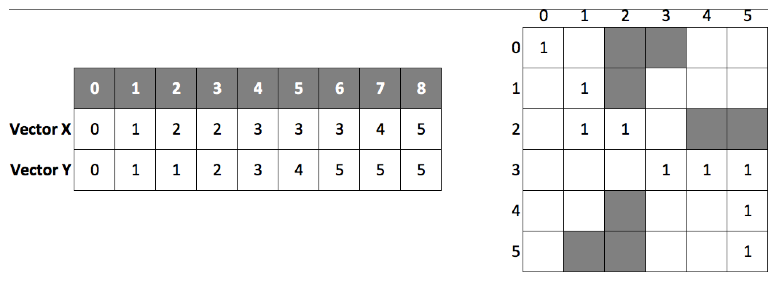
The initial solution used by the SA algorithm is created using the cumulative penalty costs matrix, where indices correspond with the point coordinates. The rectangular mesh is generated using the universal transversal Mercator (UTM) system. A greedy uninformed search procedure is used to create the initial solution encoded by two integer-valued vectors containing the coordinates of the nodes being part of the route. Figure 1 shows a candidate solution representing a path between (0,0) and (5,5) points.

The mechanism to find neighboring solutions builds pseudo-random paths between two points selected at random in the current solution. The search for alternatives routes uses a matrix of visited nodes to avoid using those that have been part of previous solutions. This procedure applies the following steps:

• Randomly select a point r₁ from s.
• Randomly select a second point r₂ from s. The distance between r₁ and r₂ cannot exceed a maximum distance previously defined.
• Copy the points of s in locations 0 to r1 − 1 in s’.
• Generate a pseudo-random path in s’ between nodes r₁ and r₂, through an informed search, giving priority to the least visited cells.
• Update the values of the cells that have been visited in the path pseudo-random between nodes r₁ and r₂.
• Copy the second part of s from locations r₂ + 1 up to n − 1 in s’.

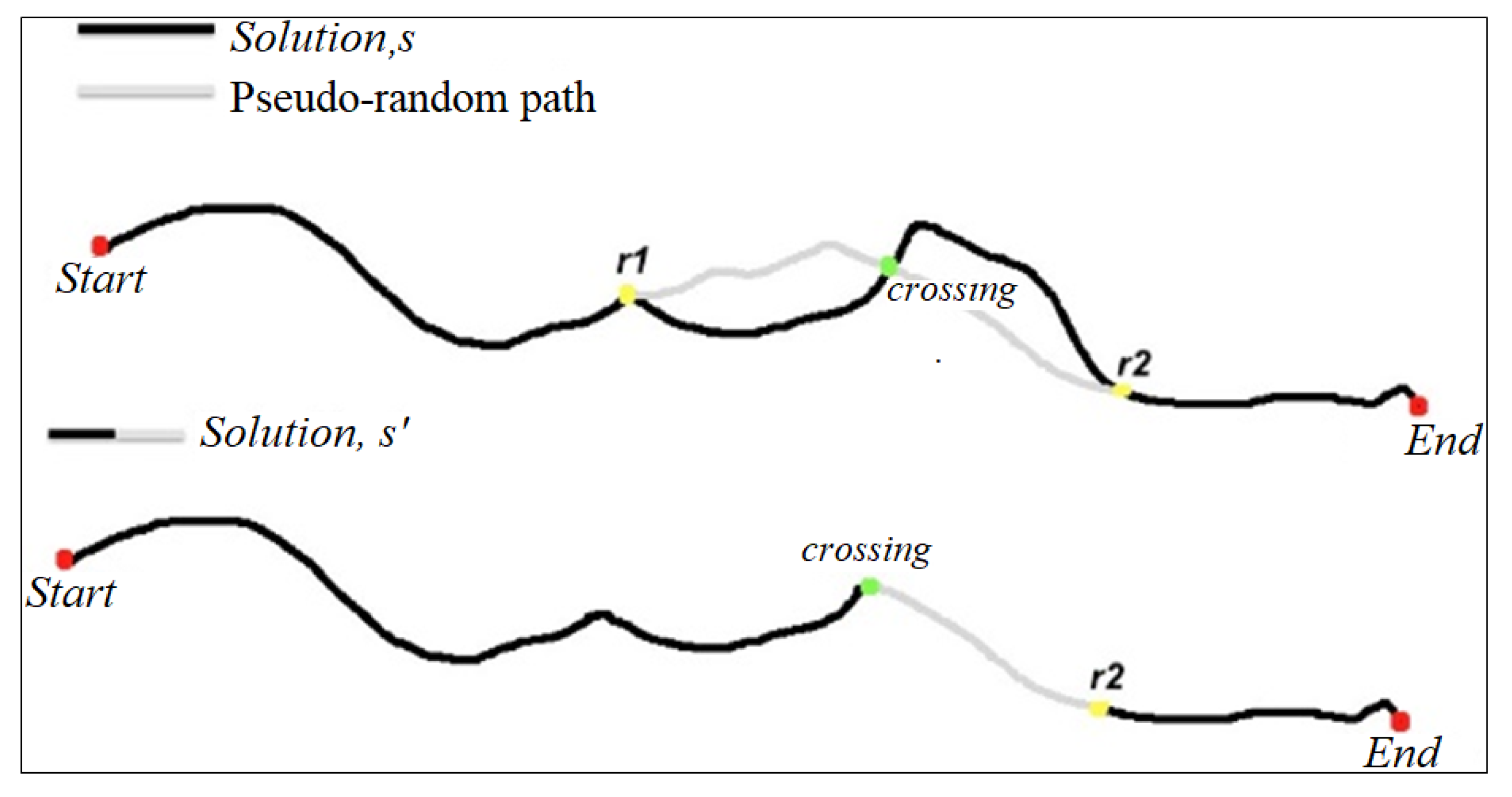
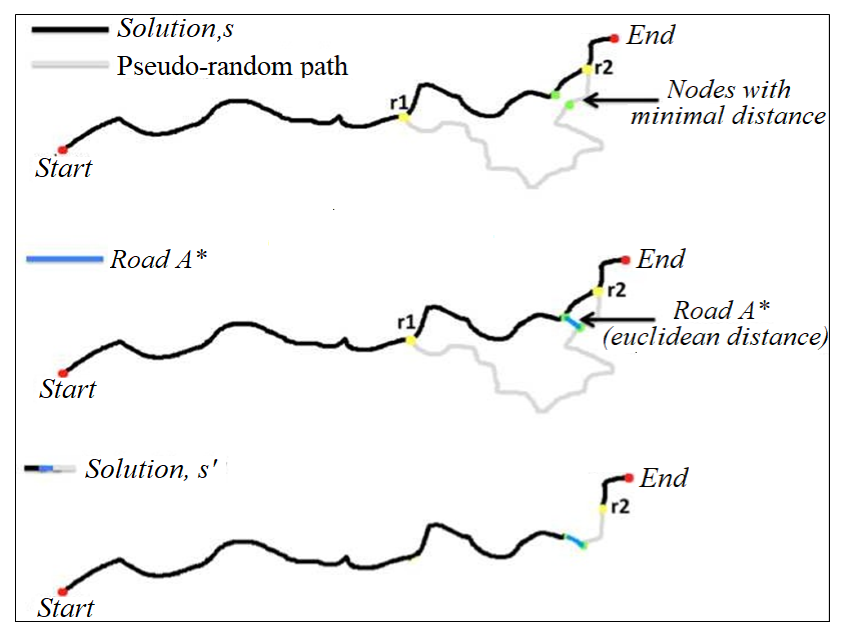
Two conditions must be considered to avoid repeated movements, considered as tabu movements in the pseudo-random paths. The first one verifies if a common point exists between s and the generated pseudo-random path. If this point exists, s’ is created by merging s with the pseudo-random path using this common point (Figure 2). The second condition is applied if the paths are not sharing a common point. To merge the two nodes closest to the r₂ point having the least distance between them are searched for to be connected through the A* heuristic [52] (Figure 3).

The matrix of visited nodes (u,v) allows extending the exploration to refine the initial trajectory through the physical restrictions existing during the search. Figure 4, shows this matrix, as well as the current solution and the pseudo-random path generated between points r₁ and r₂ in green and cyan colors, respectively.

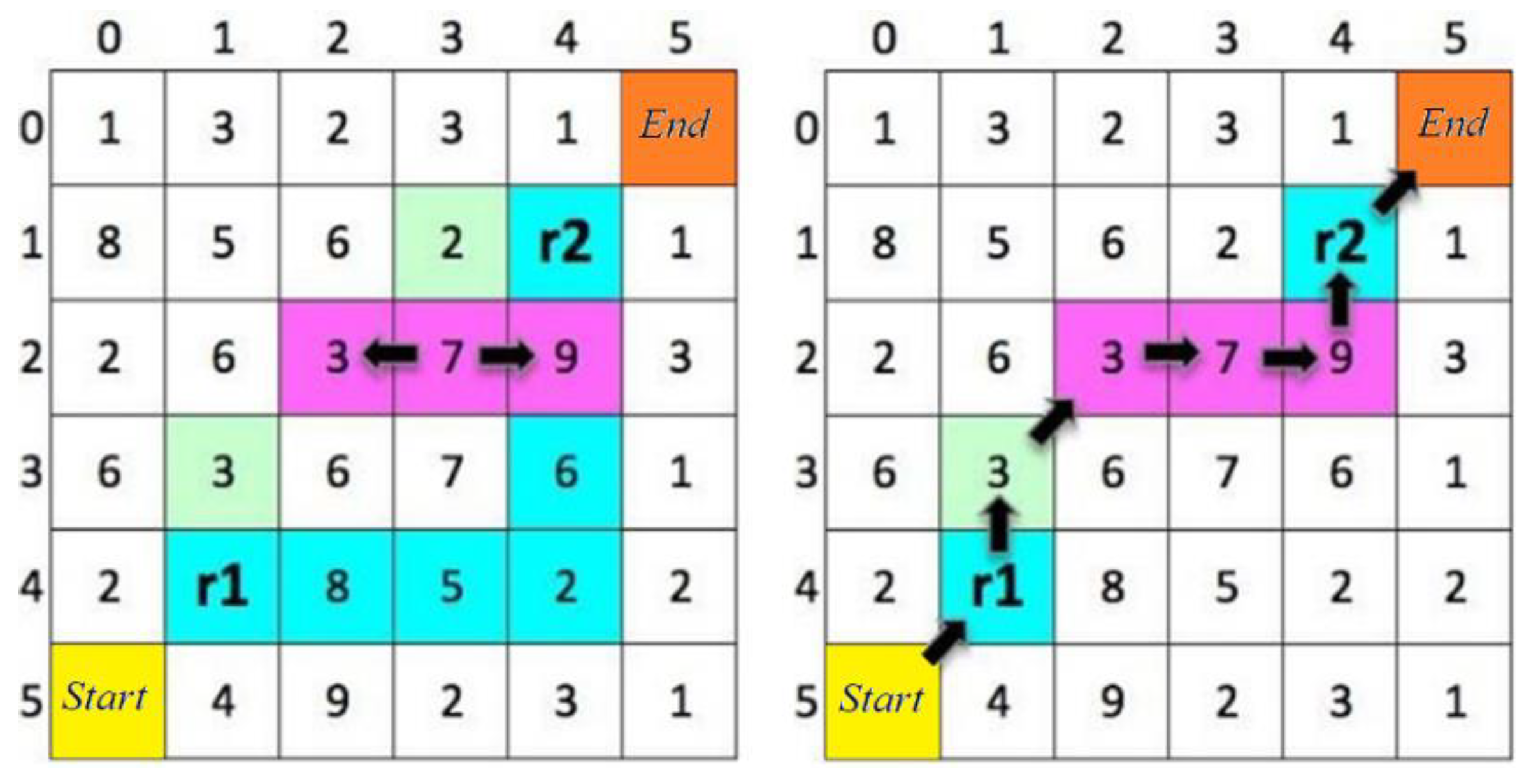
Since these paths are not sharing a common point, the second criterion is applied to create an alternative solution. First, the nearest points to r₂ are identified, and a path between them is generated using the A* algorithm. Figure 5 shows the resulting alternative solution s’, where (2,2) in the current solution and (2,4) in the pseudo-random path are the nearest points to r₂.

Figure 6 shows an example of a corridor in green color with limits in purple color. The shortest route P is shown in red color and the route P1 obtained by the SA algorithm is shown in blue color. This route is feasible since it is contained in the corridor, complying with the mathematical model’s constraint (4). The route P2 (in orange color) is infeasible since part of it is outside the corridor, and the perturbation solution (s, ptam) function is used to repair it.

Once the stop condition of the algorithm is reached, the best solution’s values are mapped to the UTM coordinates, and the corridor is displayed on the map using a GIS tool.

4. Experimental Results and Discussion

This section describes the platform used for the development of this work. First, a description of the test problems used for experimentation is presented. Next, the control parameters of the SA algorithm are shown. Finally, the experimental results are shown and the results obtained are depicted by visualizing the routes through a GIS tool.

4.1. Test Problems

Three realistic scenarios with different dimensions are tested in the proposed approach. The geographic information is provided by the National Institute of Statistics and Geography of Mexico (INEGI). INEGI organizes the information of Mexico according to map scales. The digital elevation model (DEM) and topography are used to generate the cumulative cost matrix. Figure 7 shows the organization in topographic charts of the Mexican regions at two scales (1:250,000 and 1:50,000). The 1:50,000 map scale is considered to calculate the distance of the nodes sequence p, in kilometers (km), as follows:

$$dist\left(s,t\right)=\frac{p.50}{1000}$$

(7)

For formulating the three test problems, the topographic charts shown in

Table 1. Topographic charts that correspond to each problem.

Problem Dimension	Topographic Charts
586 × 732	E14B49
585 × 1467	E14B59 Y E14B79
5341 × 6727	E14B41-49, E14B51-59, E14B61-69, E14B71-79 Y E14B81-89

are used. From these topographic charts, the maximum elevation in the area comprising the first two scenarios is 80 m above sea level, so in the present work, the half of this value (40 m) is taken as the e_max value. For the third scenario, 1/20 of the maximum elevation (5610 m above sea level) is used, so e_max is set as 280.5.

Figure 8 shows the names of the topographic charts of the Mexican territory used in this experimental study, which corresponds to the geographic information for the year 2015. The first test problem is a small network of 586 × 732 nodes covering the Mexican port of Veracruz. The second one consists of a medium-sized network of 585 × 1467 nodes, including the Joachín and Naranjos cities, both in Veracruz state, México. Finally, the third problem is an extensive network of 5341 × 6727 nodes comprising part of the Mexican states of Morelos, Guerrero, Puebla, and Veracruz.

The topographic restrictions used for the test problems are based on a classification defined by the feasibility penalties of the different topographic layers.

Table 2. Penalization of the topographic layers of problems 1 and 2.

Layer	Penalty	Layer	Penalty
Aqueduct	5	Ducts	5
Road track	6	Urban areas	8
Streets	5	Buildings	8
Bridges	10	Green areas	2
Water channel	8	Communication Inst.	7
Sub. its T. electric	9	Water bodies	8
Roads	5	Port Inst.	9
Railways	9	Ins. industrial	10
Roads	7	Communication lines	9
Airport	10	Water ponds	8
Cemeteries	8	Locations	6
Growing areas	1	Sports Inst.	9

shows the penalties used in the first two test problems and

Table 3. Penalization of the topographic layers of problem 3.

Layer	Penalty	Layer	Penalty
Aqueduct	7	Villages	9
Railroad	9	Communication paths	10
Streets	8	Sports Inst.	7
Sub. its T. electric	8	Aviation runway	9
Cemetery	9	Miscellaneous Inst.	5
Green areas	1	Locations	8
Ducts	1	Industrial Inst.	10
Water bodies	8	Bridges	7
Buildings	9	Growing areas	1

shows those used in the third one.

4.2. Parameters of the Simulated Annealing Algorithm

Due to the stochastic nature of the SA algorithm, 30 independent runs are performed on the three test scenarios to obtain experimental results. The values of the algorithm control parameters are shown in

Table 4. Tuned values of the algorithm control parameters.

Parameter	Value
T0	0.9
Tf	0.0001
β	0.98
Lmarkov	10

.

The convergence test applying the tuned values of the control parameters for problem one is shown in Figure 9. Once the control parameters are tuned with the best results, the experiments for the three previously described instances are carried out.

4.3. Experimental Results

The experimental evaluation of the SA algorithm is carried out on a computer with Intel Xeon X5675/3.07GHz CPUs and 24 GB RAM. The algorithm is implemented using the C++ language and is compiled with GCC 4.9.4 on Linux 2.6-EL5. The results obtained by the SA algorithm on each test instance are described using several tables in the following paragraphs. They indicate the best solution value found, the mean value, and the standard deviation (SD) of these executions. In this work, a greedy BFS is chosen, which does not use a cost function to explore possible routes. This solution is used as the SA initial solution, and the comparison is carried out with the BFS strategy to show the quality of solutions obtained by SA within a corridor. BFS only generates a single solution, unlike the SA algorithm, which can produce multiple optimized local solutions that do not violate the restriction of leaving the corridor. When starting the search procedure with a solution that is not the global optimum obtained by a greedy BFS, it generates alternate routes within the corridor. Otherwise, if SA is initialized with a globally optimal solution, what happens is that the paths found by SA are very similar to each other and do not extend in the corridor, limiting the search space of the algorithm. SA seeks alternative routes with great diversity, which can be adjusted to the corridor’s width.

The corridor distances obtained by both the BFS strategy and the SA algorithms are shown. The results depicted in

Table 5. Cost of the best solution with a neighborhood size of 10% of the solution s.

Problem	Greedy-BFS	SA	Average	SD
586 × 732	715	423	428.70	4.26
585 × 1467	1528	988	998.76	6.50
5341 × 6727	8335	6028	6840.60	584.55

,

Table 6. Cost of the best solution with a neighborhood size of 30% of the solution s.

Problem	Greedy-BFS	SA	Average	SD
586 × 732	715	484	496.13	4.71
585 × 1467	1528	1113	1136.8	16.34
5341 × 6727	8335	6032	7146.9	416.75

,

Table 7. Cost of the best solution with a neighborhood size of 50% of the solution s.

Problem	Greedy-BFS	SA	Average	SD
586 × 732	715	530	537.83	4.93
585 × 1467	1528	1184	1202.13	7.85
5341 × 6727	8335	5968	7212.7	584.55

,

Table 8. Cost of the best solution with a neighborhood size of 70% of the solution s.

Problem	Greedy-BFS	SA	Average	SD
586 × 732	715	545	554.23	3.4
585 × 1467	1528	1221	1235.13	6.34
5341 × 6727	8335	6004	7179.9	611.6

show the optimization that SA does with the initial solution obtained by the greedy-BFS strategy, and it is observed in the best solution found and in the average value obtained by SA. The objective of the comparison presented in these tables and Figure 10 and Figure 11 is to have a quality measure and diversity that the routes obtained by SA have throughout the length and width of the corridor. Naturally, if we compare the quality of these routes with an algorithm getting the optimal global path, these would be of lower quality or some would be close to the global optimum, but it would not have a diversity of routes in the corridor, which is the objective of this work, i.e., quality and diversity.

The pseudo-random paths are created using 10%, 30%, 50%, and 70% of the maximum length of the initial solution. The number of alternative routes generated by each execution is 452, using the values of the parameters shown in Table 4. The corridor redesign may require the generation of alternative routes to evaluate further solutions, which can be reached by modifying the algorithm parameters.

Table 5 shows the results obtained using random pseudo-paths with a maximum length of 10% of the total length of the initial solution. The distances obtained by the compared algorithms greedy–BFS vs. SA in the first problem are 35.75 and 21.15, for problem two are 76.4 and 49.4, and for problem three are 416.75 and 301.4.

Table 6 shows the results obtained using pseudo-random paths with a maximum length of 30% of the total length of the initial solution. The distances obtained by the compared algorithms are 35.75 and 24.4, 76.4 and 55.65, and 416.75 and 301.6 for the problems one, two, and three, respectively.

Table 7 shows the results obtained using pseudo-random paths with a maximum length of 50% of the total length. The distances obtained by the compared methods are 35.75 and 26.5, 76.4 and 59.2, and 416.75 for problems one, two, and three, respectively.

Finally, Table 8 shows the results obtained using pseudo-random paths with a maximum length of 70% of the total length. The distances obtained by the compared algorithms are 35.75 and 27.25, 76.4 and 61.05, and 416.75 and 306.2 for problems one, two, and three, respectively.

Figure 10 shows the behavior of the objective function concerning the size of the neighborhood structure: Figure 10a is for problem one, and Figure 10b is for problem 2.

Figure 11 shows a graphical representation of the corridors obtained by the SA algorithm for problems one (Figure 11a) and two (Figure 11b). For verifying that the solutions found by the SA algorithm are feasible, it is necessary to visualize them using a GIS. The 10% neighborhood structure allows finding better solutions with alternative routes (red routes) than the initial solution (pink routes). The neighborhood structure using 30% and 50% of the initial solution finds good solutions (green and yellow routes). Finally, the neighborhood structure using 70% of the initial solution allows refining the initial trajectory very finely (purple routes).

Figure 11 shows the routes found inside the corridor with different neighborhood structures. These routes do not follow the same path indicating that the configuration of alternate routes obtained by SA presents a good diversity of independent paths since most of the routes found coincide only in some sections, and additionally, SA allows a good quality of the local optimal solutions.

The average time required for the SA algorithm to find its best solutions are 5.38, 13.3, and 520.76 s for problems one, two, and three, respectively.

5. Conclusions and Future Work

The corridor planning problem can be addressed as an optimization problem with topological restrictions. This paper presents the SA algorithm’s implementation using a variable neighborhood mechanism to generate different alternative routes and select the best one for this problem. By using a guided pseudo-random search approach, the variable neighborhood structure explores alternative routes improving the initial solution.

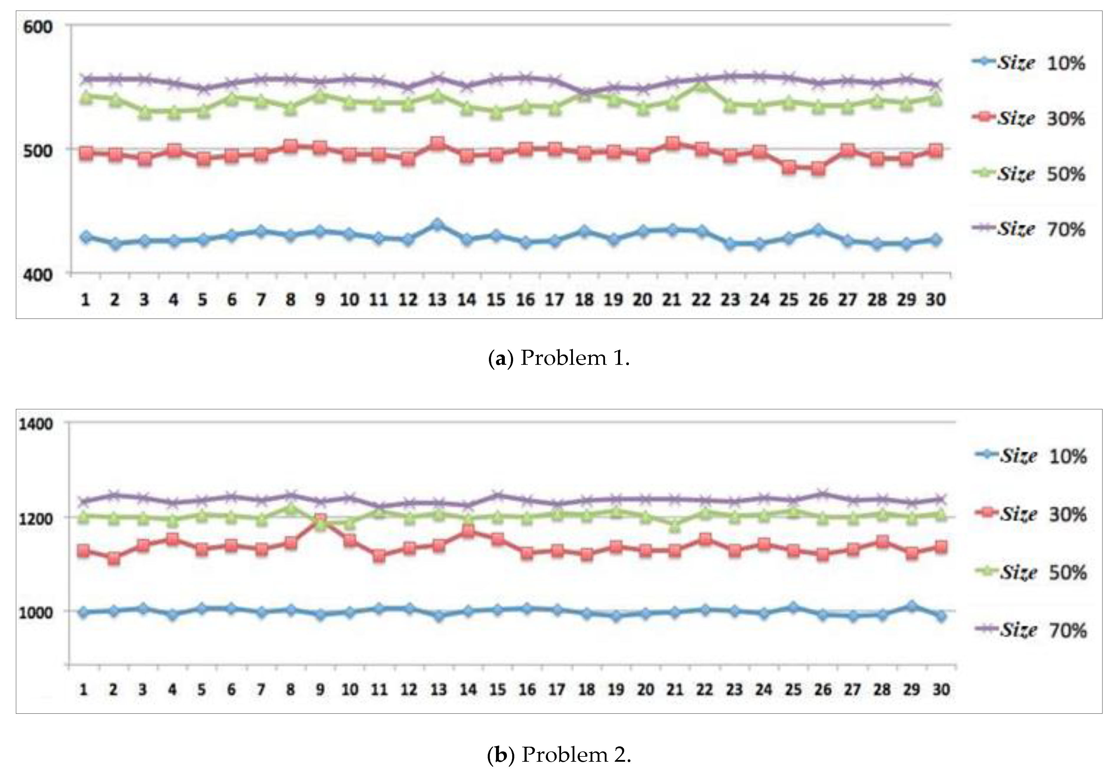
The experimental results demonstrate that implementing the proposed mechanism in SA generates alternative routes with quality and diversity. Likewise, the results obtained by the SA algorithm significantly exceeds 18% over those gotten by the greedy method, this only indicates for comparative purposes that SA obtains optimized routes, but it is not verified that SA gets the best solution. Moreover, the implementation of the proposed neighborhood mechanism outweighs the greedy algorithm in solving large-size problems. Applying a variable neighborhood mechanism in SA allows generating diversity in routes, which is important if it is necessary to choose other alternative paths that respect a corridor’s limits. With the results obtained in this work, the objective of finding routes with quality and diversity is met. The SA algorithm solves three practical problems using real topographic data. However, it can be used in a variety of problems finding the shortest route between two points on realistic scenarios.

Future work can be proposed to develop a method fitting the curves of the impact zone (strip) of the corridor to narrow the search. In this way, it is allowed to explore different alternate routes relatively close to the initial solution without getting too far away. For improving the computation time used to generate an initial solution, it is proposed to implement the techniques used in the MOGADOR method and look for other random mechanisms generating a feasible initial solution in the shortest possible time. The problem needs to be addressed as a multi-objective optimization problem. In addition, it is possible to parallelize the method by its vector nature and the optimization algorithm.

Something very important for future work is to work on problems by dynamically varying the values of the layers so that the costs of the links change depending on the set of selected links, adapting a greedy uninformed search strategy, the breadth-first-search (BFS) algorithm with the same neighborhood structure procedures used in this work to find multiple solutions and focus on finding multiple global optimal paths.

Finally, many real problems have GIS information in different formats and scales that could make the spatial analysis complicated. However, it is possible to convert the different data models to a raster format, adapt the different scales to perform complex spatial analysis, and exploit the geographic information available in diverse private and public sources.

References

1. Miller, H.; Shih-Lung, S. Geographic Information Systems for Transportation in the 21st Century. Geogr. Compass 2015, 9, 180–189. [Google Scholar] [CrossRef]
2. Goodchild, M.F. An evaluation of lattice solutions to the problem of corridor location. Environ. Plan. A 1977, 9, 727–738. [Google Scholar] [CrossRef]
3. Medrano, F.A.; Church, R.L. Corridor Location for Infrastructure Development: A Fast Bi-objective Shortest Path Method for Approximating the Pareto Frontier. Int. Reg. Sci. Rev. 2013, 37, 129–148. [Google Scholar] [CrossRef]
4. Church, R.L.; Loban, S.R.; Lombard, K. An interface for exploring spatial alternatives for a corridor location problem. Comput. Geosci. 1992, 18, 1095–1105. [Google Scholar] [CrossRef]
5. Bell, M.G.H.; Iida, Y. Transportation Network Analysis; Wiley: Chichester, UK, 1997. [Google Scholar]
6. Zhang, X.; Armstrong, M.P. Genetic Algorithms and the Corridor Location Problem: Multiple Objectives and Alternative Solutions. Environ. Plan. B Plan. Des. 2008, 35, 148–168. [Google Scholar] [CrossRef] [Green Version]
7. Turner, A.K.F. Computer-Assisted Procedures to Generate and Evaluate Regional Highway Alternatives, Tech Report No. 32; Purdue University: West Lafayette, IN, USA, 1968. [Google Scholar]
8. Lombard, K.; Church, R.L. The gateway shortest path problem: Generating alternative routes for a corridor location problem. Geogr. Syst. 1993, 1, 25–45. [Google Scholar]
9. Scaparra, M.P.; Church, R.L.; Medrano, F.A. Corridor location: The multi-gateway shortest path model. J. Geogr. Syst. 2014, 16, 287–309. [Google Scholar] [CrossRef]
10. Fournier, E.D. MOGADOR revisited: Improving a genetic approach to multi-objective corridor search. Environ. Plan. B Plan. Des. 2015, 43, 663–680. [Google Scholar] [CrossRef]
11. Dijkstra, E.W. A note on two problems in connexion with graphs. Numer. Math. 1959, 1, 269–271. [Google Scholar] [CrossRef] [Green Version]
12. Miller, H.; Shih-Lung, S. Geographic Information Systems for Transportation, Principles and Applications; Oxford University Press: Oxford, UK, 2001. [Google Scholar]
13. Kishore, T.S.; Singal, S.K. Optimal economic planning of power transmission lines: A review. Renew. Sustain. Energy Rev. 2014, 39, 949–974. [Google Scholar] [CrossRef]
14. Medrano, F.A. Corridor Location: Generating Competitive and Efficient Route Alternatives. Ph.D. Thesis, University of California, Santa Barbara, CA, USA, 2014. [Google Scholar]
15. Hong, I.; Murray, A.T. Efficient measurement of continuous space shortest distance around barriers. Int. J. Geogr. Inf. Sci. 2013, 27, 2302–2318. [Google Scholar] [CrossRef]
16. Johnson, P.E.; Joy, D.S.; Clarke, D.B.; Jacobi, J.M. HIGHWAY 3.1: An enhanced HIGHWAY Routing Model: Program Description, Methodology, and Revised User’s Manual; Oak Ridge National Lab.: Oak Ridge, TN, USA, 1993.
17. Yen, J.Y. Finding the K Shortest Loopless Paths in a Network. Manag. Sci. 1971, 17, 712–716. [Google Scholar] [CrossRef]
18. Byers, T.H.; Waterman, M.S. Technical Note—Determining All Optimal and Near-Optimal Solutions when Solving Shortest Path Problems by Dynamic Programming. Oper. Res. 1984, 32, 1381–1384. [Google Scholar] [CrossRef] [Green Version]
19. Kuby, M.; Zhongyi, X.; Xiaodong, X. A Minimax Method for Finding the k Best “Differentiated” Paths. Geogr. Anal. 1997, 29, 298–313. [Google Scholar] [CrossRef]
20. Akgün, V.; Erkut, E.; Batta, R. On finding dissimilar paths. Eur. J. Oper. Res. 2000, 121, 232–246. [Google Scholar] [CrossRef]
21. Aissi, H.; Chakhar, S.; Mousseau, V. GIS-based multicriteria evaluation approach for corridor siting. Environ. Plan. B Plan. Des. 2012, 39, 287–307. [Google Scholar] [CrossRef]
22. Medrano, F.A.; Church, R.L. A Parallel Algorithm to Solve Near-Shortest Path Problems on Raster Graphs. In Modern Accelerator Technologies for Geographic Information Science; Shi, X., Kindratenko, V., Yang, C., Eds.; Springer: Boston, MA, USA, 2013; pp. 83–94. [Google Scholar]
23. Carlyle, W.M.; Wood, R.K. Near-shortest and k-shortest Simple Paths. Networks 2005, 46, 98–109. [Google Scholar] [CrossRef]
24. Hallam, C.; Harrison, K.J.; Ward, J.A. A Multiobjective Optimal Path Algorithm. Digit. Signal Process. 2001, 11, 133–143. [Google Scholar] [CrossRef]
25. Jong, J.C.; Jha, M.K.; Schonfeld, P. Preliminary highway design with genetic algorithms and geographic information systems. Comput. Civ. Infrastruct. Eng. 2000, 15, 261–271. [Google Scholar] [CrossRef]
26. Jha, M.K.; McCall, C.; Schonfeld, P. Using GIS, genetic algorithms, and visualization in highway development. Comput. Civ. Infrastruct. Eng. 2001, 16, 399–414. [Google Scholar] [CrossRef]
27. Jong, J.C.; Schonfeld, P. An evolutionary model for simultaneously optimizing three-dimensional highway alignments. Transp. Res. Part B Methodol. 2003, 37, 107–128. [Google Scholar] [CrossRef]
28. Tat, C.W.; Tao, F. Using GIS and Genetic Algorithm in Highway Alignment Optimization. In Proceedings of the 2003 IEEE International Conference on Intelligent Transportation Systems, Shanghai China, 12–15 October 2003; Volume 2, pp. 1563–1567. [Google Scholar]
29. Al-Hadad, B.M.A. Corridor Based Horizontal Highway Alignment Optimization Using GIS and Genetic Algorithms. Eurasian J. Sci. Eng. 2018, 4, 98–116. [Google Scholar]
30. Jha, M.K.; Schonfeld, P.; Samanta, S. Optimizing rail transit routes with genetic algorithms and geographic information system. J. Urban Plan. Dev. 2007, 133, 161–171. [Google Scholar] [CrossRef]
31. Samanta, S.; Jha, M.K. Modeling a rail transit alignment considering different objectives. Transp. Res. Part A Policy Pr. 2011, 45, 31–45. [Google Scholar] [CrossRef]
32. Isler, C.A.; Widmer, J.A. Parallel Genetic Algorithm and High Performance Computing to Solve the Intercity Railway Alignment Optimization Problem. In Sustainable Rail Transport; Springer: Cham, Switzerland, 2020; pp. 159–186. [Google Scholar]
33. Maji, A.; Jha, M.K. Multi-objective highway alignment optimization using a genetic algorithm. J. Adv. Transp. 2009, 43, 481–504. [Google Scholar] [CrossRef]
34. Yang, H.; Zhao, L.; Xu, J. Multi-Objective Optimization Model of Highway Alignment. In Proceedings of the 2011 IEEE 3rd International Conference on Communication Software and Networks, Xi’an, China, 27–29 May 2011; pp. 585–590. [Google Scholar]
35. Aruga, K.; Sessions, J.; Akay, A.; Chung, W. Simultaneous optimization of horizontal and vertical alignments of forest roads using Tabu Search. Int. J. For. Eng. 2005, 16, 137–151. [Google Scholar] [CrossRef]
36. Romero, D.; Sanchez-Flores, A. The One-Dimensional Space Allocation Problem: A Simulated Annealing Approach. In Advances in Numerical Partial Differential Equations and Optimization; Gómez, S., Ed.; Society for Industrial & Applied Mathematics: Philadelphia, PA, USA, 1991. [Google Scholar]
37. Shafahi, Y.; Bagherian, M. A customized particle swarm method to solve highway alignment optimization problem. Comput. Civ. Infrastruct. Eng. 2013, 28, 52–67. [Google Scholar] [CrossRef]
38. Sushma, M.B.; Roy, S.; Prasad, M.B.R.; Maji, A. Optimum Point of Intersection Selection in Horizontal Highway Alignment Design: A Comparative Study Using Path Planner Method and Ant Algorithm. In Transportation Research; Springer: Singapore, 2020; pp. 185–199. [Google Scholar]
39. Douglas, D.H. Least-cost Path in GIS Using an Accumulated Cost Surface and Slopelines. Cartogr. Int. J. Geogr. Inf. Geovisualization 1994, 31, 37–51. [Google Scholar] [CrossRef]
40. Berry, J.K. Map Analysis: Understanding Spatial Patterns and Relationships; GeoTec Medi: San Francisco, CA, USA, 2007. [Google Scholar]
41. Olaya, V. Sistemas de información geográfica. Cuad. Int. Tecnol. Para Desarro. Hum. 2009, 8, 15. [Google Scholar]
42. Huber, D.L.; Church, R.L. Transmission Corridor Location Modeling. J. Transp. Eng. 1985, 111, 114–130. [Google Scholar] [CrossRef]
43. Kirkpatrick, S.; Gelatt, C.D.; Vecchi, M.P. Optimization by Simulated Annealing. Science 1983, 220, 671–680. [Google Scholar] [CrossRef] [PubMed]
44. Kirkpatrick, S. Optimization by simulated annealing: Quantitative studies. J. Stat. Phys. 1984, 34, 975–986. [Google Scholar] [CrossRef]
45. Geman, S.; Geman, D. Stochastic relaxation, Gibbs distributions, and the Bayesian restoration of images. IEEE Trans. Pattern Anal. Mach. Intell. 1984, PAMI-6, 721–741. [Google Scholar] [CrossRef]
46. Moreno-Bernal, P.; Cruz-Chávez, M.A.; Rodríguez-León, A.; Lopez, O.; Malumbres, M.P.; Martínez-Rangel, M.G.; Juarez-Chavez, J.Y. Simulated Annealing Algorithm for 2D Image Compression. In Proceedings of the 2012 IEEE Ninth Electronics, Robotics and Automotive Mechanics Conference, Cuernavaca, Mexico, 19–23 November 2012; pp. 129–134. [Google Scholar]
47. Talbi, E.G. Metaheuristics: From Design to Implementation; John Wiley & Sons: Hoboken, NJ, USA, 2009. [Google Scholar]
48. Metropolis, N.; Rosenbluth, A.W.; Rosenbluth, M.N.; Teller, A.H.; Teller, E. Equation of State Calculations by Fast Computing Machines. J. Chem. Phys. 1953, 21, 1087–1092. [Google Scholar] [CrossRef] [Green Version]
49. Cruz-Chavez, M.A.; Martinez-Oropeza, A.; Barquera, S.S. Neighborhood Hybrid Structure for Discrete Optimization Problems. In Proceedings of the 2010 IEEE Electronics, Robotics and Automotive Mechanics Conference, Cuernavaca, Mexico, 22–25 September 2009; pp. 108–113. [Google Scholar]
50. Guttmann, A.J. On two-dimensional self-avoiding random walks. J. Phys. A Math. Gen. 1984, 17, 455–468. [Google Scholar] [CrossRef]
51. Domb, C. Self-Avoiding Walks on Lattices. In Advances in Chemical Physics; John Wiley & Sons, Ltd.: Hoboken, NJ, USA, 2007; pp. 229–259. [Google Scholar]
52. Hart, P.E.; Nilsson, N.J.; Raphael, B. A formal basis for the heuristic determination of minimum cost paths. IEEE Trans. Syst. Sci. Cybern. 1968, 4, 100–107. [Google Scholar] [CrossRef]
Figure 1. Vectors representing the initial solution.
Applsci 10 06190 g001
Figure 2. First exchange criterion.
Applsci 10 06190 g002
Figure 3. Second exchange criterion.
Applsci 10 06190 g003
Figure 4. Initial solution s and pseudo-random path between r1 and r2 in the matrix of visited nodes.
Applsci 10 06190 g004
Figure 5. Distance between nodes and s connection and the pseudo-random path to create s’.
Applsci 10 06190 g005
Figure 6. Corridor’s layout.
Applsci 10 06190 g006
Figure 7. Topographic charts at scales (a) 1:250,000, and (b) 1:50,000.
Applsci 10 06190 g007
Figure 8. Topographic charts of the study area.
Applsci 10 06190 g008
Figure 9. Solution cost (distance) depending on the temperature.
Applsci 10 06190 g009
Figure 10. Behavior of the objective function.
Applsci 10 06190 g010
Figure 11. Alternate routes for corridors.
Applsci 10 06190 g011