Investigation of Fluid-Structure Interaction Induced Bending for Elastic Flaps in a Cross Flow

Abstract

With the recent increase in the design of light and flexible structures, numerical investigations of fluid and structure together play a significant role in most engineering applications. Therefore, the current study presents an examination of fluid-structure interaction involving flexible structures. The problem is numerically solved by a commercial software ANSYS-Workbench. Two-way coupled three-dimensional transient simulations are carried out for the flexible flaps of different thicknesses in glycerin for a laminar flow and Reynolds number ranging from 3 < Re < 12. The bending line of the flaps is compared with experimental data for different alignments of the flaps relative to the fluid flow. The study reports the computation of the maximum tip-deflection and deformation of flaps fixed at the bottom and mounted normal to the flow. Additionally, drag coefficients for flexible flaps are computed and flow regimes in the wake of the flaps are presented. As well, the study gives an understanding on how the fluid response changes as the structure deforms and the model is appropriate to predict the behavior of thick and comparatively thinner flaps. The results are sufficiently encouraging to consider the present model for analyzing turbulent flow processes against flexible objects.

1. Introduction

Fluid-structure interaction (FSI) states the mutual interaction of a structure with a flowing fluid and develops the fluid and solid motions and the dependency of these motions on each other. Such kind of problems involve, the velocity and pressure of fluid effects and are affected by the structure deformation. In recent years, it has become a prominent characteristic of various engineering projects because design involves lighter and more flexible structures. The conduct of these structures with a fluid generates multi physical situations which are usually complex to handle. Numerical calculations play an important role in most engineering areas and have become more challenging due to the prediction of different flow regimes which cannot be seen in experiments (EXP) but it is still a challenge to have accurate numerical simulation of a FSI problem because of strong fluid-structure coupling. FSI problems are ever present in nature for example flapping wings, flags [1,2,3,4,5,6,7,8,9], aquatic animals [10], flexible vegetation [11,12,13], in hemodynamics [1,14] and human hair and hair sensors [15]. Thin structures are of great interest for microfluidic procedures in engineering and biomedical applications [16,17,18] and structural dynamics [18,19,20].

For investigating fluid motion together with the structure, extensive theoretical, experimental and numerical studies across flexible plates are carried out in the context of plate flapping, vibration, flutter instability, the effect of wake on plate stability and the estimation of natural frequency for plates exposed to axial flow directions [21,22,23,24,25]. Results indicate that the flapping amplitude of the plate is mainly controlled by the elastic modulus and density ratio whereas frequency is a function of length-thickness ratio and density ratio. Also with an increase in Reynolds number, the plate indicates the transfer of symmetric to asymmetric flapping [21]. The forcing amplitude is the major influence on the plate resonance while flow velocity and plate bending rigidity indicate only the minor effect providing the forcing frequency is normalized with the natural frequency of the plate [10].

Aside from flat plates in axial flow direction, research work is offered to examine a vertical bottom-fixed flat plate in a laminar boundary layer. A study representing the Reynolds number, structure-to-fluid mass ratio and bending of the plate, respectively, determine the dynamic behavior of the flexible plate. Based on this, a two-dimensional (2D) numerical study [26] presents the dynamic response of a flexible plate engrossed in laminar condition for Reynolds numbers of 100, 200, 400 and 800 by an immersed boundary method (IBM). The dynamics of the plate indicate that the plate is stable for a low Reynolds number; however, when the Reynolds number reaches 800, the plate starts vibrating. The effect of bending rigidity, ranging from 0.1–1.6, demonstrates the periodic vibrations of the plate at low values and chaotic vibration when bending rigidity approaches between 0.2 and 0.4, then switching to periodic vibration again for a bending rigidity of 0.8 and 1.6. In comparison with the flapping flag [27], the plate shows a considerably different response in terms of frequency and vibrations.

The interaction of severely deformed structures with their environment is significant in many life science applications and technical systems. Nevertheless, precise and stable numerical methods for illustrating such problems are still exceptional. Tian et al. [28] developed a coupling between an existing immersed boundary flow solver together with a nonlinear finite element (FE) solver. Furthermore, they evaluate six practical applications of FSI specifically for three dimensions (3D), which primarily have large deformations. Considering a flexible plate as one of the test examples, the free-end deflection and drag coefficients measurements for Reynolds numbers ranging from 100–1600 with and without the effect of gravity and buoyancy forces are presented. Initially, the results of the baseline case with experimental data [29] are compared and then new simulations are offered for future benchmark cases. Moreover, the plate test case is used as a model to investigate the dynamic interaction of aquatic plants. The method overall leads to a numerical stability for all test cases.

The dynamic changes in the structure could possibly affect many aspects of fluid forces and present interesting fluid performance. Therefore, it is an important aspect for multiphase flow industrial applications. To compute such problems, tip-displacement of a rubber beam in a two-phase flow of air and oil was examined using a two-way coupled FSI [30]. A benchmark case [31] was simulated and previously published data of simulations and experiments were compared in terms of beam tip-deflection. The difference between 2D and 3D simulations has been clearly explained as well.

A scheme that has treated the deflection line of single and tandem beam configurations is presented by Axtmann et al. [32]. It is attained by interacting both experiments and direct numerical simulations (DNS) for Reynolds numbers ranging from 1–60 in a viscous fluid. Bending is calculated via beam bending theory. Bending lines of simulations and experiments demonstrate a good agreement for both single and tandem arrangements. A prediction model for cross flow velocity is offered. Moreover, local drag coefficient along pillar is computed and an empirical model based on drag coefficient is tested and proposed. Furthermore, a two-way coupled FSI study for different rows of flexible flaps is conducted to investigate the wavering behavior at the tip of flaps and development of vortices in the gap among the flaps. Experiments have been performed for water and glycerin against the silicon rubber flaps, reaching the maximum Reynolds number of 120, and the resulting tip-deflection of flaps is compared experimentally and numerically [5].

Investigating transient directional deformations of flexible obstacles by means of different numerical algorithms has been a subject of various studies involving the relevance of the extended arbitrary Langrangian Eulerian (ALE) method [33] and monolithic solvers [34,35]. The test problems presented [33] can be used as a benchmark for the formulation of numerical problems involving 2D FSI with immersed structures that have large displacements. While 2D benchmark cases, free-surface flows and test cases of an elastic obstacle and plate have been presented for monolithic approaches and validated with other numerical methods [34,35]. Similarly, for the analysis of hemodynamic problems, a new and more sophisticated computational formulation named immersed structural potential method (ISPM), based on the original IBM, is presented. The novel method accounts for the computation of FSI force field at the fluid mesh and description of cardiovascular tissue scheme by viscoelastic fiber-reinforced constitutive models. A new time-integration method is also introduced for the computation of a deformation gradient tensor. Three advancement cases of deformable cylinders and flapping membranes are presented. The study is applicable for highly complex FSI problems incorporating large deformations under pulsating flows and sinking and floating rigid bodies [36]. To describe the deflection of flaps and moving boundaries, the fluid- solid interface-tracking/interface-capturing technique (FSITICT) is applied to the FSI problem with ALE interface tracking and Eulerian interface tracking. The method is demonstrated by test FSI cases. First, test computations are performed for two flapping membranes and the second test case is composed of one flapping membrane and a movable, elastic arterial-structure. The flapping membranes and fluid are modelled in fully Eulerian coordinates in both test cases, while the elastic structure in the second case is computed in Lagrangian coordinates. The overall objective is to reduce the computational cost and test the applicability of the method for large deformations in order to analyze different cardiac cycles [37].

In the light of the above survey, it is concluded that the previous research efforts are made to encounter the dynamics of flapping structures in uniform flows. Prediction of the bending line and tip-displacement of a flexible flap fixed at the bottom in 3D is rarely seen in the literature. With the simple geometry of a flap in a rectangular fluid domain, the problem is fundamental in nature and can be used in applications that coincide with the flow, forcing functions and the solid boundary conditions. Therefore, this study emphasizes on the deformation characteristics of the flaps over time, flap bending positions and different flap orientations. The focus of this study is to explore the motion of an elastic flap immersed in a rectangular fluid domain and to analyze the bending of flexible structures in 3D under laminar flow conditions.

This paper is organized as follows-first, an insight into experimental procedure is presented then a computational model is demonstrated in terms of different flap thicknesses and positions. Later, the response of flexible flaps is analyzed in terms of bending and deformation in addition, the results of flap bending are offered in comparison with the experimental work. The effect of the different clamping angles is discussed as well. Similarly, the computation of drag coefficient at various clamping positions is a part of the current research. Flow regimes are revealed at various time steps and velocity contours in the wake are shown. Finally, some discussions are presented.

2. Material and Method

A numerical two-way FSI model is presented for validating the towing-tank experimental data for flexible flaps. For the validation purposes, transient structure (flap) and unsteady flow are modeled using a commercial software ANSYS-Workbench. Each field is demonstrated separately by defining its geometry, properties, mesh, boundary conditions and respective solvers. Coupling is introduced between individual domains to establish a two-way FSI.

The experimental and numerical setups, settings and conditions are presented in the following subsets.

2.1. Experiments

A summary of the experimental data is given in the present section, whereas detail can be found in the reference [32]. Flaps of different thicknesses are fixed in the center of a plate and immersed into the working fluid.

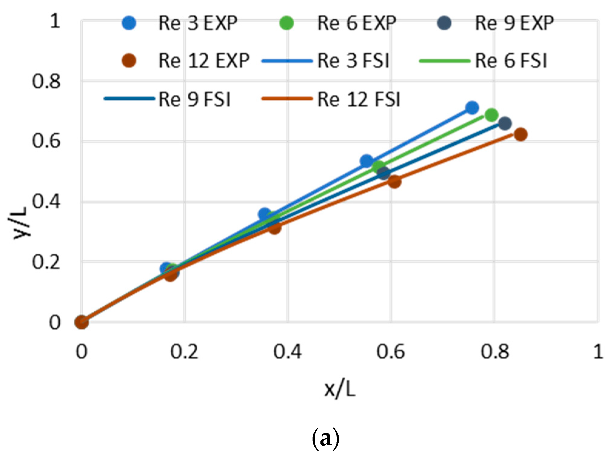
Flaps are designed with length of 100 mm, width of 20 mm and thicknesses of 5 and 10 mm. Several measurements for the deformable flaps are taken by varying the flow conditions (Reynolds number, Re = 3 to 12) and flap arrangements that is, at clamping angles from 0° to 90° and inclined angle of 45°. The bending of the flaps was recorded for each case. As the effective Reynolds number is small and viscous forces are dominating, only bending response is observed in the experiments instead of vortex shedding, which would cause periodic vibrations.

2.2. Numerical Model

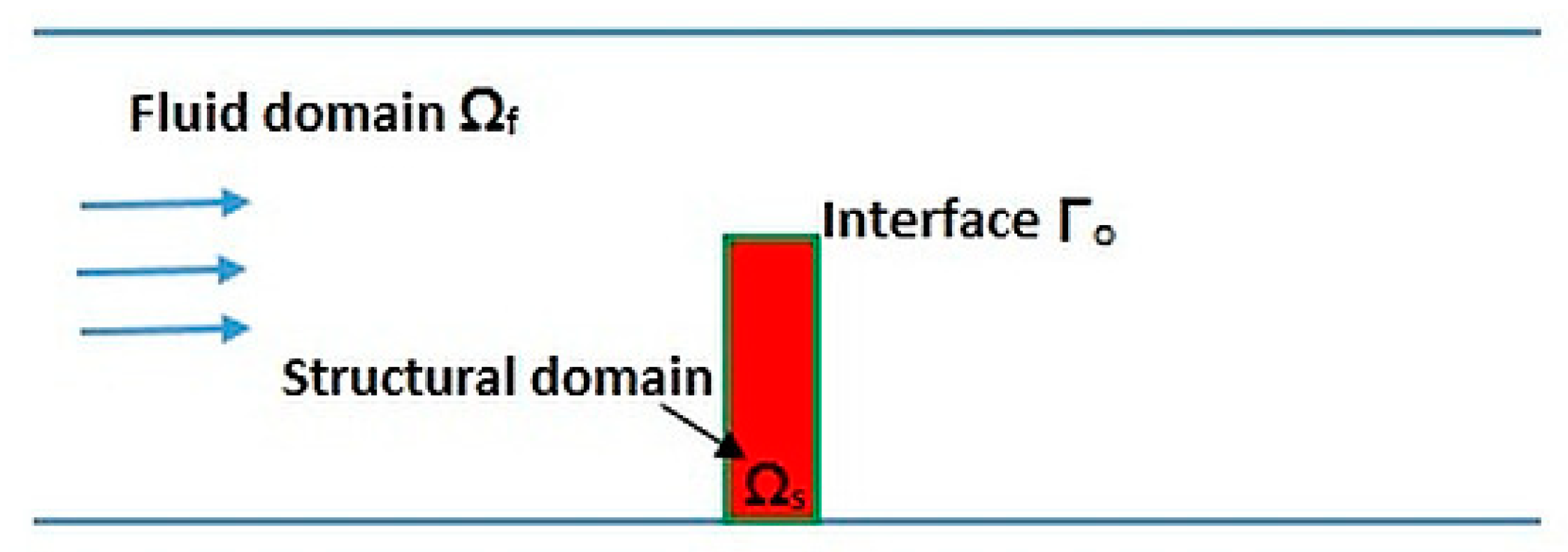
FSI modeling mainly deals with the information about how the fluid domain acts as a function of structure and how structural domain behaves as a function of fluid domain, at the interface, information is shared between the structural and fluid solver thus founding FSI [38]. In the present case, an elastic structure was surrounded by incompressible Newtonian fluid flow. Ω_f(t) is defined as a time dependent fluid domain and Ω_s(t) is defined as a time dependent structural domain. It is assumed that for all the time t, Ω_f(t) is entirely occupied by the fluid and Ω_s(t) is entirely occupied by the structure. Besides, Γ_o(t) = Ω_f(t) ∩ Ω_s(t) is an interface where the elastic structure interacts with the fluid. A schematic of FSI in terms of structural domain, fluid domain and interface for a present case of an elastic flap immersed in a rectangular fluid domain is shown in Figure 1.

For the established FSI solution, the kinematic, dynamic and geometric conditions at the common interface of fluid and structure should be satisfied, numerically at the interface Γ_o(t), the following conditions are assumed for all the time t:

$$v_i^s=v_i^f$$

(1)

$${\sigma }_{ij}^{s }{n}_{i }={\sigma }_{ij}^f n_i.$$

(2)

Here, $v^s$ and $v^f$ represent the structure and fluid velocity constituting the kinematic stability. Dynamic stability is attained by the continuous normal stresses of solid ${\sigma }^s$ and fluid ${\sigma }^f$ at the interface.$n$ being the unit vector normal at the interface and the subscript i indicates its direction. According to the geometric condition stability fluid-solid domain always match and do not overlap [38].

Equations of motion for the structure and fluid are expressed as follows:

Structure equations

The flexible flap is modeled as an elastic continuum therefore the balance of linear momentum is given by:

$${\rho }^s \dot{v_i^s}={\sigma }_{ij,j}^s \mathrm{in} {\mathsf{\Omega }}_{\mathrm{s}}(\mathrm{t}).$$

(3)

For linear elastic material, the linear Hook’s law is followed by the structural stress as:

$${\sigma }_{ij}^s=2H{\epsilon }_{ij}+\lambda {\epsilon }_{kk}{\delta }_{ij},$$

(4)

where ${\rho }^s$ is the structural density and ${\sigma }_{ij.j }^s$ is the structural stress. The subscript ij of the stresses in Equations (3), (4), (6) and (7) represents the components of stress tensor whereas the subscript j, indicates the differential term involved in the linear elastic model.

The structural stress is a function of strain $\epsilon$ and the Lamé parameters $H$ and λ, which are defined as:

$$\begin{array}{l}{\epsilon }_{ij}=\frac{1}{2}\left(u_{i.j}+u_{j,i}\right)\\ H=\frac{E}{2\left(1+ѵ\right)}\\ \lambda =\frac{Eѵ}{\left(1+ѵ\right)\left(1-2ѵ\right)},\end{array}$$

where $u$ represents the displacement, $E$ and $ѵ$ are Young’s modulus and Poisson ratio, respectively [38,39,40].

Fluid equations

The governing equations for time-dependent fluid regime are modeled by incompressible continuity and Navier-Stokes equations in terms of velocity $v^f$, static pressure $P$ and fluid density ${\rho }^f$ as follows [38,39,40]:

$$\mathrm{div} {\dot{v}}_i^f= 0 \mathrm{in} {\mathsf{\Omega }}_{\mathrm{f}}(\mathrm{t})$$

(5)

$${\rho }^f \dot{v_i^f}={\sigma }_{ij,j}^f \mathrm{in} {\mathsf{\Omega }}_{\mathrm{f}}(\mathrm{t}).$$

(6)

The fluid stress for an incompressible fluid is simplified to:

$$\begin{array}{r}{\sigma }_{ij}^f=-P{\delta }_{ij}+{\tau }_{ij}\\ {\tau }_{ij}=\frac{2}{3}\mu \left(e_{ij}-{\delta }_{ij}{e}_{kk}\right)\\ e_{ij }= \left(v_{i.j}^f+v_{j,i}^f\right).\end{array}$$

(7)

The dynamic mesh motion for an FSI problem is defined in terms of arbitrary movement of the grid points with respect to their frame of reference by considering the convection of the material points. The material derivative in terms of the movement of fluid mesh can be expressed as [40]:

$$\frac{d{v}^f}{dt}= \frac{\partial v^f}{\partial t}+\left(v^f -U\right)· \nabla v^f,$$

(8)

where $U$ is the mesh movement of fluid, also $U$ = $K U_{sur}$ representing $K$ as a stiffness matrix of an elastic media and $U_{sur}$ being the fluid dynamics surface mesh movement.

Modeling of structure and fluid in ANSYS-Workbench are explained in the following sections:

2.2.1. Structural Model

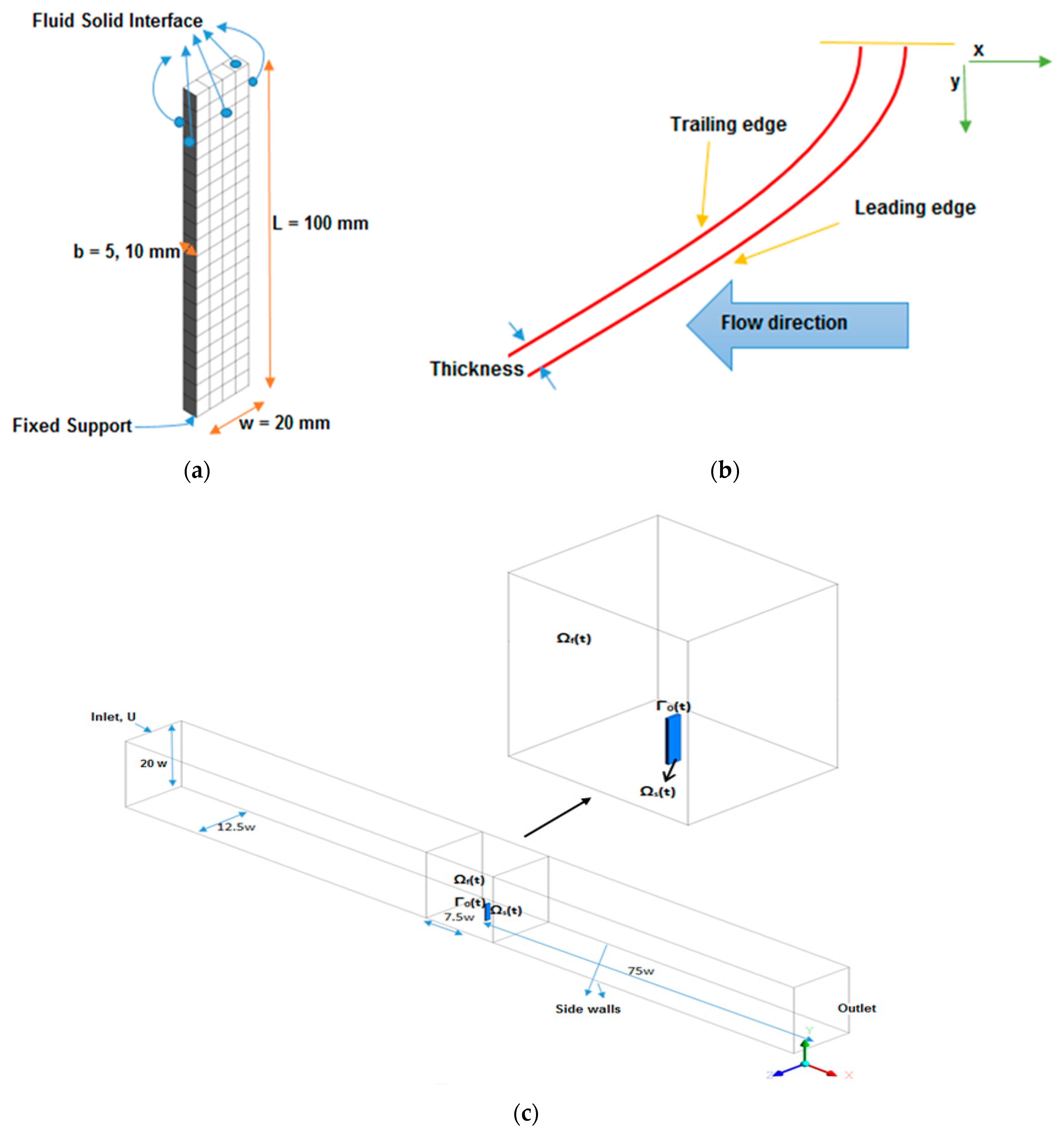
The solid model is designed in ‘Transient Structural’ (ANSYS-Mechanical) by a (FE) analysis, afterwards the geometry is defined in the ANSYS Design Modeler. To estimate the flow as close as possible to the experiments, all dimensions and parameters are needed to be precisely defined according to the experimental setup and can be seen in

Table 1. Engineering parameters and dimensions.

Fluid-Glycerin	Density, ${\mathsf{\rho }}^{\mathrm{f}}$	1220 kg/m3
	Dynamic viscosity, $\mathsf{\mu }$	1 kg/m s
Structure-Flap	Length, L	100 mm
	Width, w	20 mm
	Thickness, b	5 mm, 10 mm
	Density, ${\mathsf{\rho }}^{\mathrm{s}}$	1030 kg/m3
	Young’s modulus,$\mathrm{E}$	1.23 MPa
	Poisons ratio, $\mathrm{v}$	0.3
	Shear modulus, G	0.473 MPa

.

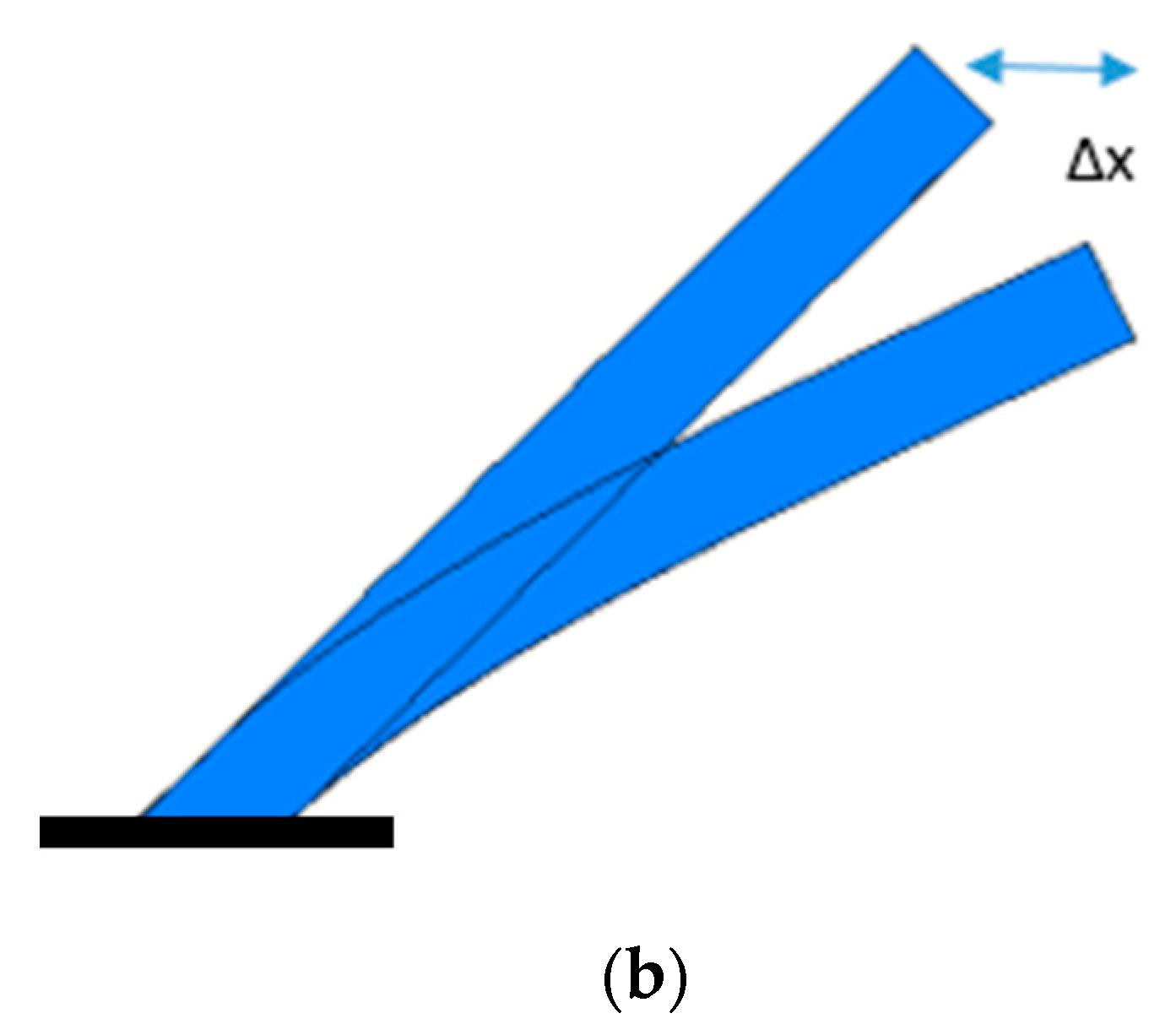
Analogous to the experiments, the structural model is considered as a flexible flap that is, the bottom wall is fixed, while all other walls are free. The fixed wall is assigned as ‘Fixed support’ whereas the remaining part of the flap is given the ‘Fluid Solid Interface.’ The flap is meshed by hexahedral elements and are depicted in Figure 2a. Specifying ‘w = 0.02 m’ being the width of the flap and height as 5 w, the flap is positioned at 7.5 w (center) of the plate and 6.25 w from the side walls, whereas the distance of the flap from outlet is specified as 75 w. Accordingly, the rectangular flow domain is indicated as (150w, 20w, 12.5w). The structural model and FSI domain are shown in Figure 2a–c respectively. Part (a) of the figure represents the flap, its dimensions, mesh and transient conditions, (b) indicates the bending definitions and (c) shows the collected computational domain of fluid and structure.

2.2.2. Computational Model

The fluid domain is modeled by ANSYS-FLUENT for flaps immersed in a glycerin environment as depicted in Figure 2c. Because of the low Reynolds number range, a laminar fluid model is chosen. For an effective simulation in comparison to the experiments, a fixed coordinate system is used. The constant flow velocity as ‘velocity inlet’ is given for the input conditions, plate and flap are assigned as walls with a ‘no slip’ boundary condition while the top walls, remaining bottom parts and sides are assigned as ‘slip walls’ and ‘pressure outlet’ is defined for 0 Pa at the outlet conditions. A non-dimensional Reynolds number Re is defined as Re = $v$w/υ based on the flow velocity $v$, flap width w and fluid kinematic viscosity υ. The inlet flow velocities, $v,$ ranging from 0.125–0.5 m/sec are given as input values based on the identified Reynolds number. The engineering parameters used for the computations are listed in Table 1. Due to subsonic incompressible flow field, pressure based solver with coupled scheme is used and second order implicit transient formulation is employed for modeling the unsteady flow.

Five mm thick flap:

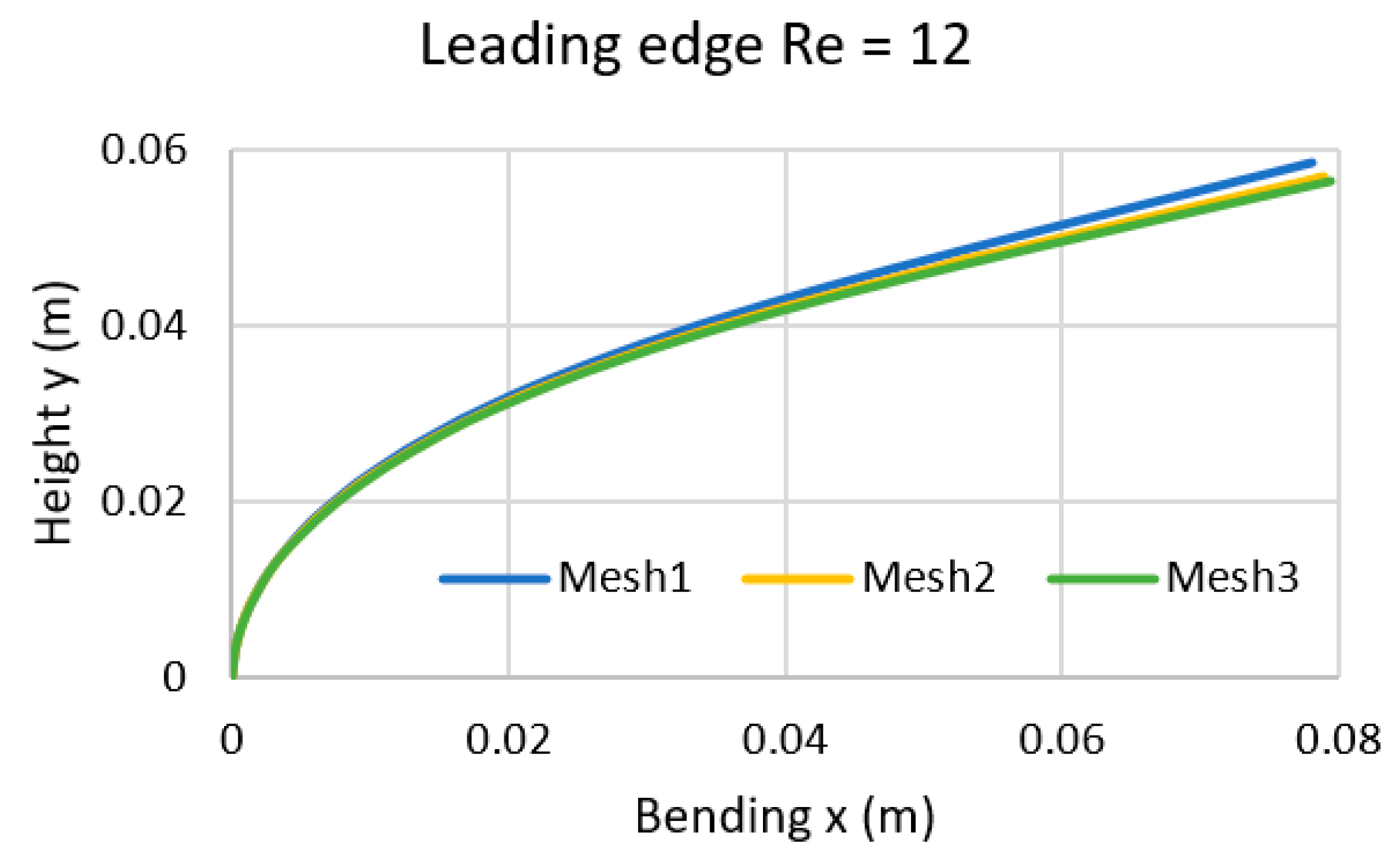
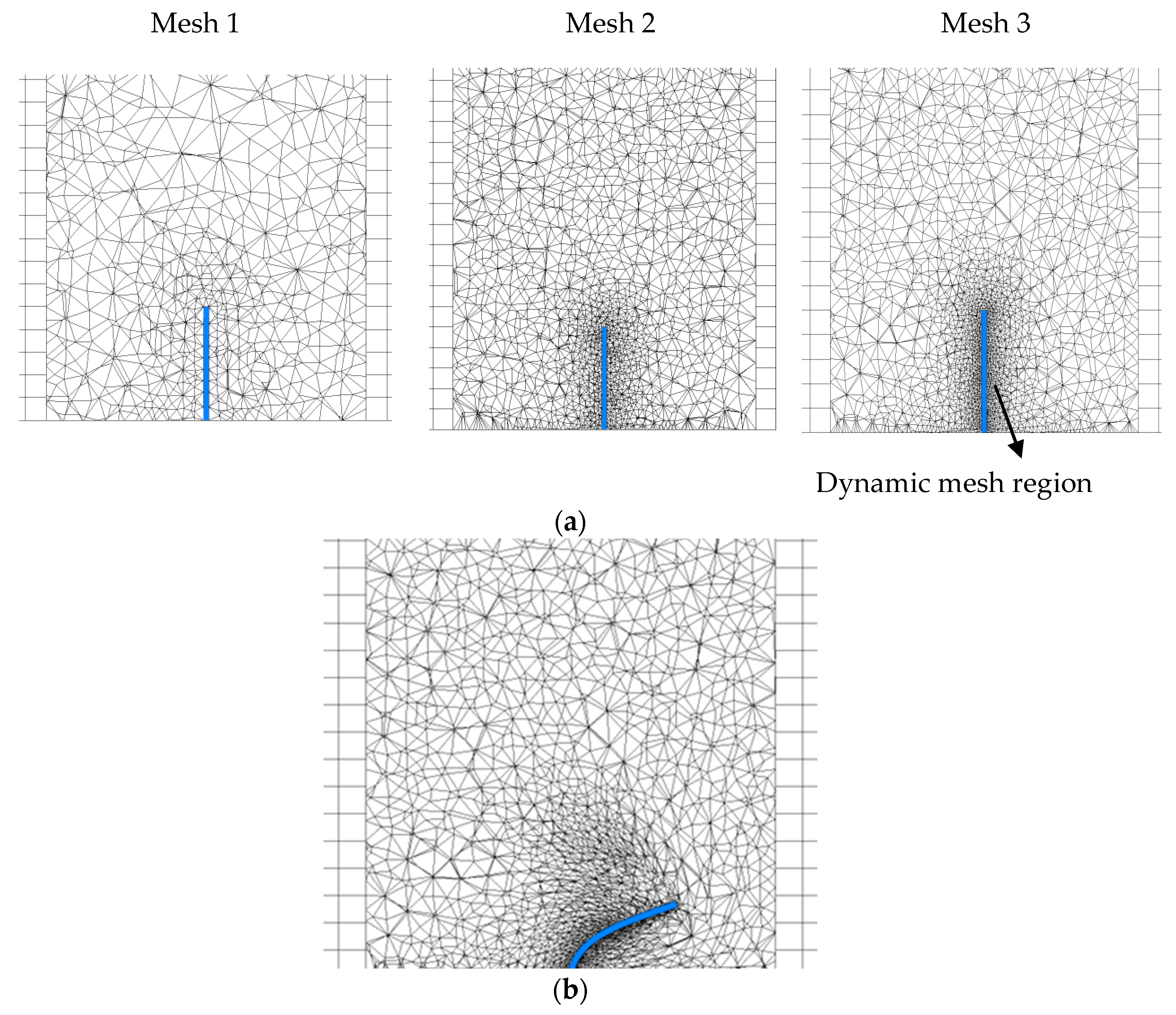
Initially, simulations were performed for a flap of 5 mm thickness. To consider mesh independence, three different meshes were tested to explore the effect of mesh resolution on a flap bending. This mesh resolution was needed to compensate for the effect of computational time such as the computational time increasing after coupling the computational fluid dynamics (CFD) and FEA models [41]. Bending line convergence for different meshes was attained with coarser to finer: mesh 1: 52,486 elements, mesh 2: 101,641 elements and mesh 3: 137,693 elements. So, mesh 3 was chosen for the final solution, although this number of elements may vary since flap deforms and dynamic meshing takes place. 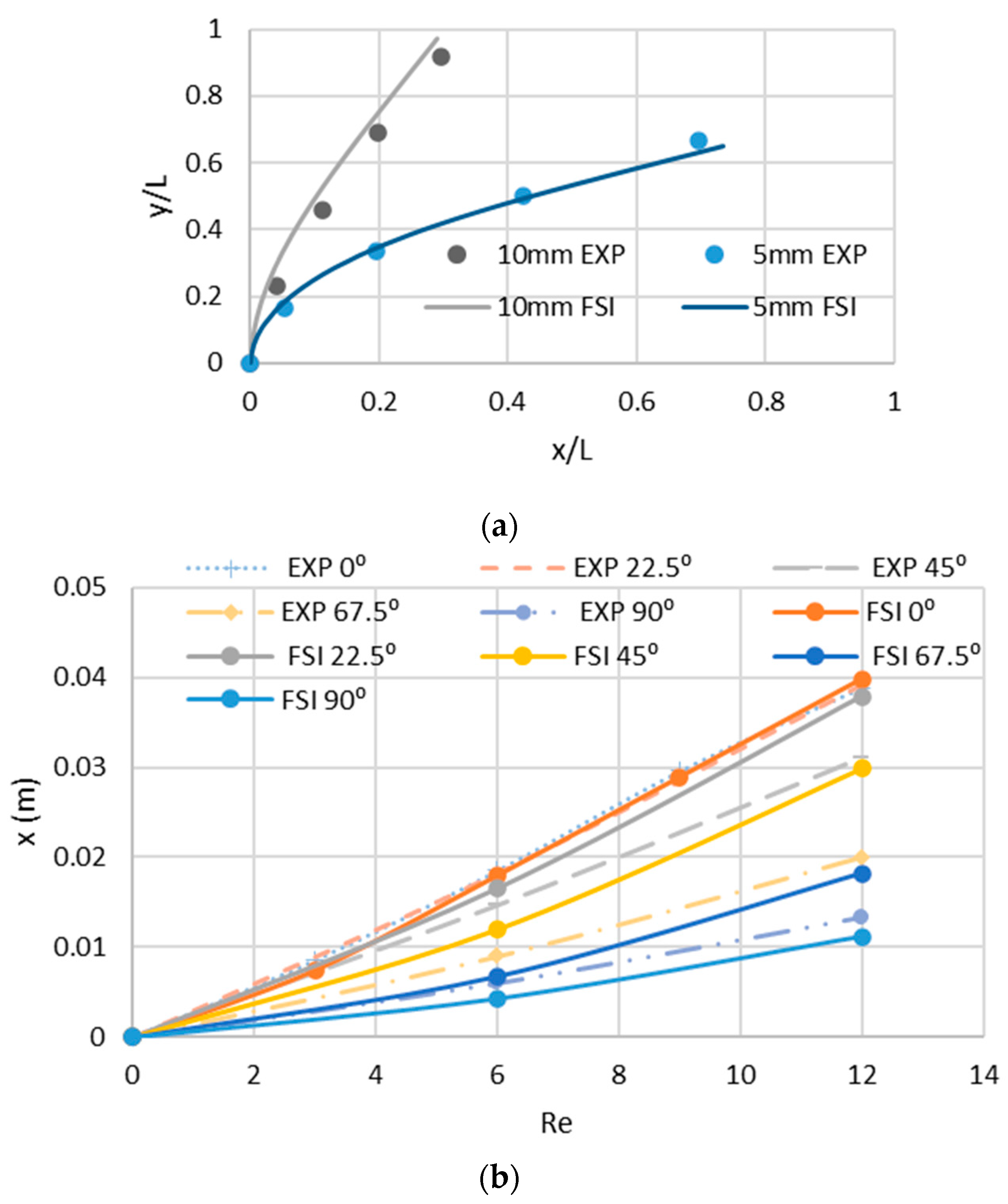Bending convergence is shown in Figure 3 whereas different meshes before and after flap deformations are depicted in Figure 4. Moreover, the difference between results obtained with mesh 2 and 3 is small, showing that grid convergence is attained. The difference between mesh 2 and 3 in terms of bending x and height y is 0.53% and 1.1% respectively.

As the large fluid domain is present, it is only desirable to have high mesh resolution around the flap and the dynamic mesh region in order to have influence of pressure and deformation gradient. For a 3D dynamic mesh domain in Fluent, a structured mesh cannot be applied [41]. For that reason, a tetrahedron unstructured mesh was chosen around the flap, though the rest of the fluid domain was designed as a structured mesh. To simulate the flap movement, both smoothing and remeshing methods were used in the dynamic mesh region such that the displacement of the flap was large compared to the grid size. Dynamic meshing is needed for both surface and volume mesh in 3D cases and it is necessary to retain element quality for both surface and volume meshes otherwise simulations may result in errors and computational differences [41]. Considering remeshing parameters, mesh scale information was followed and a minimum cell size of 6 × 10⁻⁴ m and a maximum cell size of 0.04 m were used as input values. In addition, the interface is allocated as ‘system coupling’ in dynamic mesh zones under dynamic mesh settings with a cell thickness of 0.6 mm along the wall. To provide a balance among stable mesh movement and total computational time, a time step Δt of 0.001 s is used for the coupled FSI problem for 2 s of physical flow time where the flap attained the steady-state condition.

Ten mm thick flap:

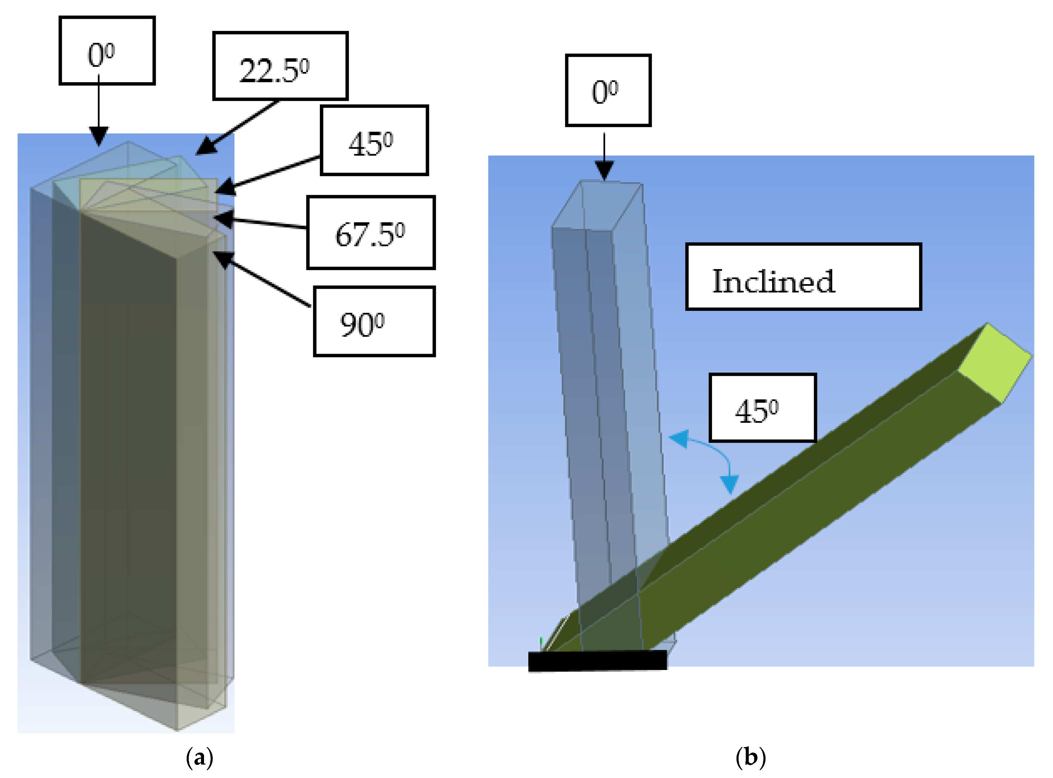
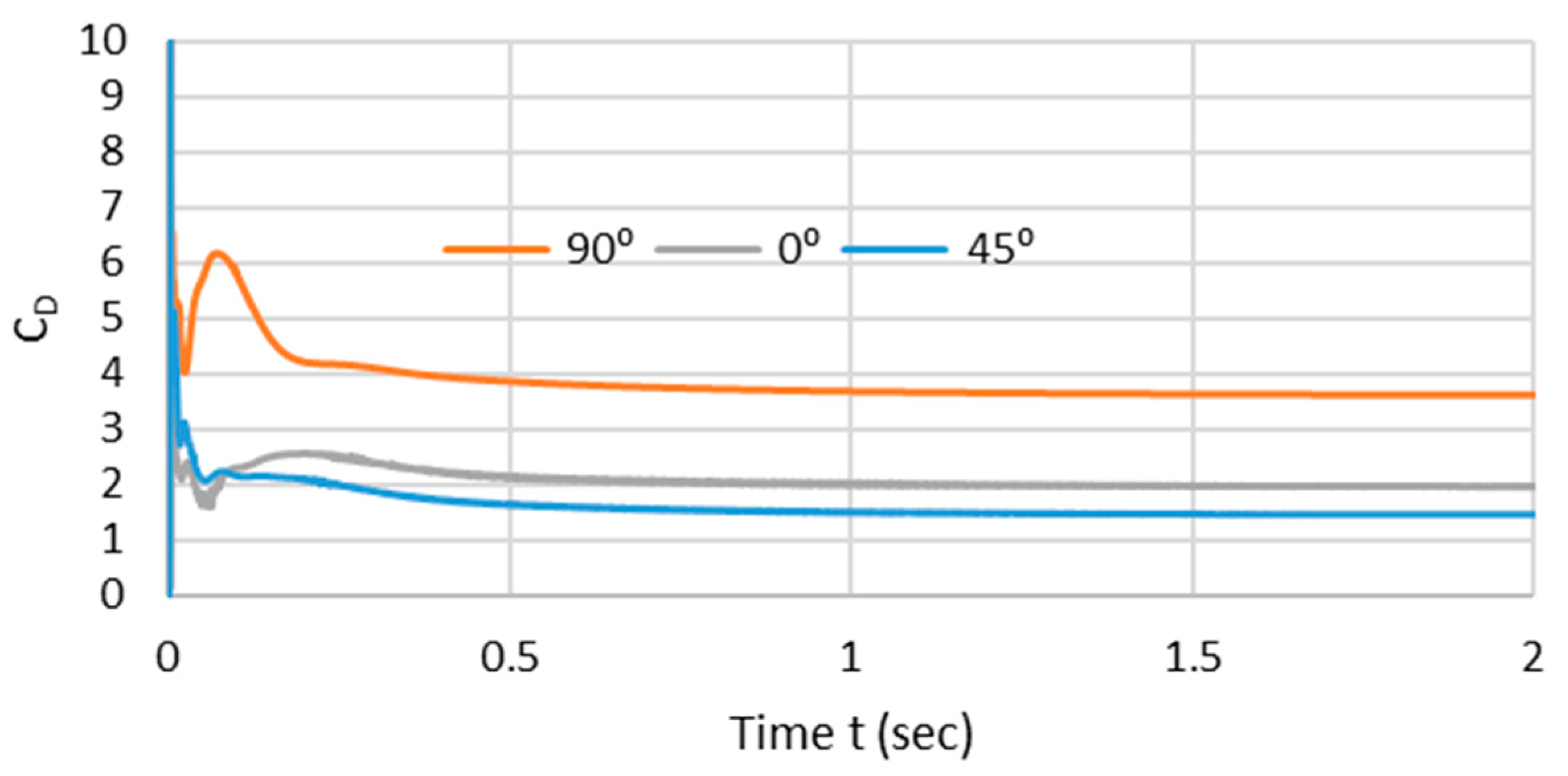
In order to meet the experimental conditions, FSI analysis for a 10 mm thick flap is performed for different flap orientations, that is, varying the clamped angle from 0° to 90°-for the angle of 0° the flap width is facing the flow, correspondingly angles are changed from 0°–90°. At 90°, the flap is rotated completely and is parallel to the flow direction. Analysis is also performed for an inclined angle of 45°. The 10 mm flap is modeled by the same structural mesh conditions as a 5 mm thick flap. Also for the fluid domain, the same mesh parameters are employed. Though the total number of elements vary in the range of 137,000–140,000 for different angles. The same boundary conditions and models are specified for 10 mm as described for the 5 mm thick flap. However, minimum and maximum length scales of remeshing differ, depending upon the flap positioning. Flap orientations designed in Design Modeler are shown in Figure 5a,b where (a) shows the different clamping positions for angle 0°–90° and (b) indicates inclined position of the flap with the angle of 45°.

3. Results and Discussions

3.1. 5 mm Thick Flap

A comparison between FSI and the experimental bending of a flap at different Reynolds numbers is expressed in Figure 6a–c. For maximum flow velocity of $\mathrm{v}$ = 0.5 m/sec (Re = 12) the flap bending is near to 1/2 of the flap length that is, y/L ≈ 0.5, for both FSI and experimental results. The simulated bending line represents the deflection of the flap in terms of x and y coordinates after reaching a steady-state. The flap bending increases with an increase in Reynolds number. However, a non-linear connection between flap deflection and Reynolds number is identified. Computational results can be taken for the whole flap length, though for the simplicity of measurements, five displacement points are measured along the length of the flap in experiments. In simulations, the x-coordinate bends to a maximum of x = 0.079 m and x = 0.076 m for leading edge and trailing edge respectively while in experiments, it is measured to be x = 0.070 m for leading edge and x = 0.067 m for the trailing edge. The results from experiments and simulations show the same bending behavior and are in good agreement. For the highest velocity, bending curves for both leading and trailing edge are shown in the Figure 6a,b, whereas the remaining results are focused only on leading edge of the flap.

Time-dependent total deformation curve of an elastic flap is processed by ANSYS-Transient Structural. Total deformation consists of directional deformations, d, in all three directions that is, X, Y and Z for a given flap. Resultant deformation varies with time from smallest to highest Reynolds number till it reaches its maximum value and then becomes constant. The deformation curves for all four Reynolds numbers at a physical flow time of 2 s after reaching steady-state can be seen in Figure 7 while Figure 8 indicates the flap visualization versus time till reaching steady-state for a Reynolds number of 9. The deformation is influenced by the magnitude of inflow velocity that is, maximum structural deformation occurs at the tip of the flap and has a least value for Reynolds 3 and increases by 0.0449 m reaching the peak value of 0.0982 m for a Reynolds number of 12. Besides, less computational time is required by the flap for the higher velocity flow in converging to the steady-state value. Thus the FSI model consists of the observations for the maximum deflections offered by the flap.

3.2. 10 mm Thick Flap

As described in Section 2.2.2, a flap of 10 mm thickness is used to simulate experimental data with different clamping orientations. For the highest Reynolds number of 12, the maximum deformation for a 10 mm thick flap is 0.53 times the 5 mm thickness for angle 0°. However, it continues to decrease with increase in the clamping angle and shows the least at 90° which is 0.37 times the deformation at clamping angle of 0°. Similarly, as the Reynolds number and the clamping angle increases, the x-coordinate of flap bending decreases indicating the minimum flap deflection with highest clamping angle (see Figure 9b) that is, the maximum x-coordinate for angle 0° is ∆x = 0.039m whereas for 90° it bends to x = 0.011 m. Similarly, a small flap deflection is also observed for inclined angle of 45°. Deformation at each position can be seen in

Table 2. Deformation across flap orientations.

Angle (°)		Maximum Transient Deformation d (m)
Clamping angle	0	0.0526
-	22.5	0.0519
-	45	0.0463
-	67.5	0.0316
-	90	0.0196
Inclined	45	0.0247

as well. Likewise, the comparison of experimental and computational results at various flap positions are shown in Figure 9 and Figure 10 respectively.

3.3. Drag Coefficient

For flow around solid bodies, the drag coefficient is defined as [42]:

$$C_D=\frac{F_D}{\frac{1}{2}\rho v^{2}S},$$

where $F_D$ is the drag force exerted by the fluid on the body and $\rho$ is the fluid density, S is the body area perpendicular to the flow direction and v is the velocity of the flow. For the present simulations, the drag coefficient, C_D, for three representative flexible flap cases is computed, that is, for a flap with a thickness of 10 mm and the clamping angles of 0°, 90° and the inclined angle of 45° at a Reynolds number of 12. The frontal area of the flap facing the flow is defined for drag calculations meant for a current 3D case. Figure 11 represents the variation of drag coefficients versus time. The mean C_D during t = 1.5–2 s for clamping angle of 90° is 3.61 and 1.95 for clamping position of 0°. Whereas for an inclined angle of 45° it is smaller than the other two cases and gives a mean of 1.45. It appears that the more bended flap is a smaller obstacle to the flow and therefore reduces the resistance from the mainstream. Moreover, the drag coefficient values are comparable with a benchmark case of a flexible flat plate in a cross flow [28].

3.4. Flow Regimes

The velocity evaluation along with flap position for thickness 5 and 10 mm intended for clamped angle 0° and Reynolds 12 is displayed in the present section at various time steps. As discussed above (Section 3.2) and shown in Figure 12, the first two time steps at t = 0.05 s and 0.1 s corresponds to the initial deflection of the flap for both thicknesses. Nevertheless, the maximum deformation reached by the 10 mm thick flap is less for the 5 mm thick flap and attained in less time, whereas, for 5mm thickness, the flap continues to bend and attain steady-state at approximately t = 1 s.

The steady-state 3D configurations of clamping angle 0°, 90° and inclined angle 45° at maximum inlet velocity is shown in Figure 13a–c presenting the region behind the flap where the transient bending converges to a steady-state and no flow fluctuation occurs downstream of the flap. The position of the flexible flap for the specified angles has changed from being straight to deformed. Flap wake indicates the absence of vortex shedding as observed in experiments because of a low Reynolds number range. Moreover, the flow past the flap is shown and compared for Reynolds numbers of 6 and 12 for clamping angle of 90° in Figure 13d,e and also for 5 mm thick flap representing the flow for minimum and maximum Reynolds number in Figure 13f,g, respectively. The higher Reynolds number leads to the higher velocity of the flow at the flap-tip and further downstream in the wake of the flap. Besides, the maximum bending of the flap in Figure 13g bends the streamlines near the flap downstream.

4. Discussion

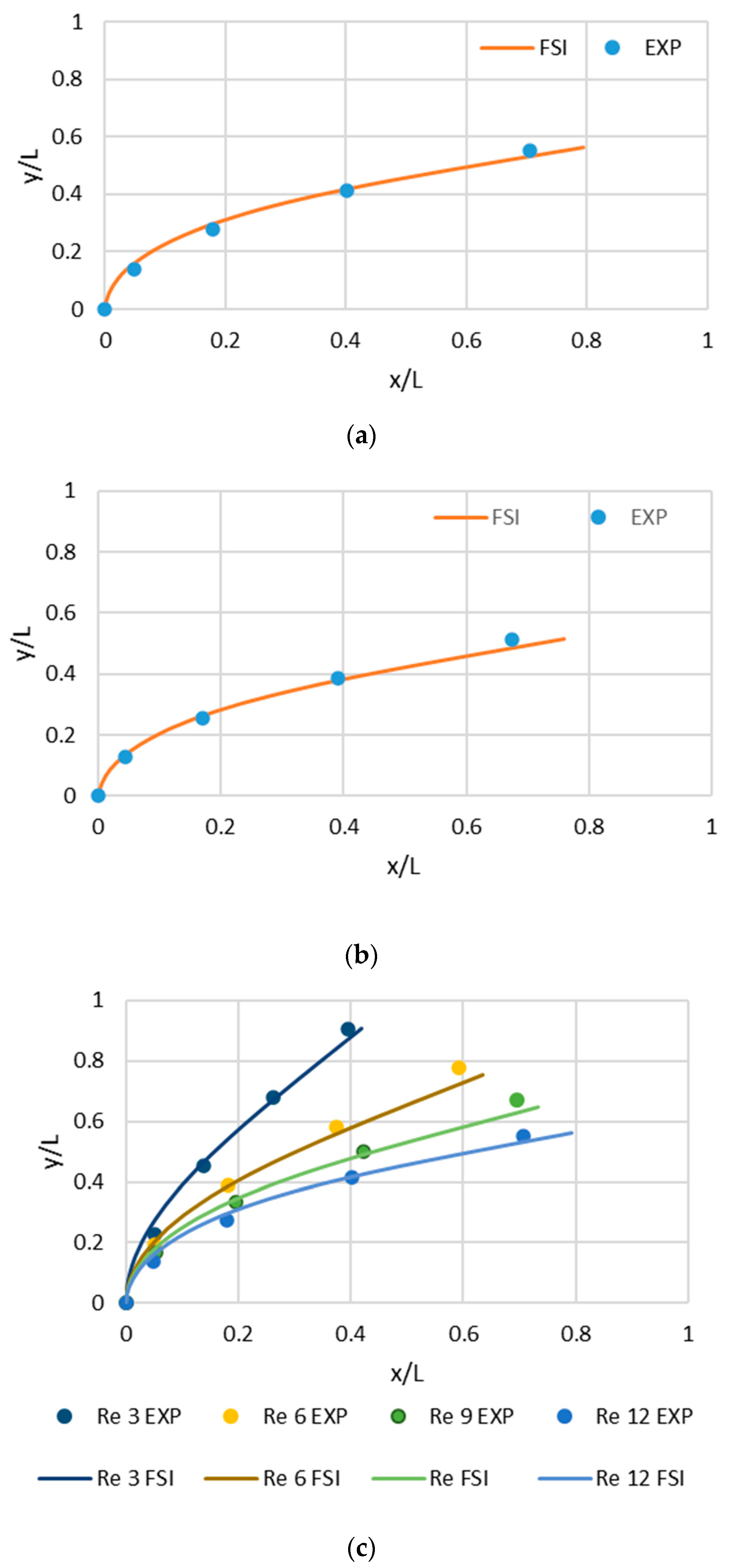
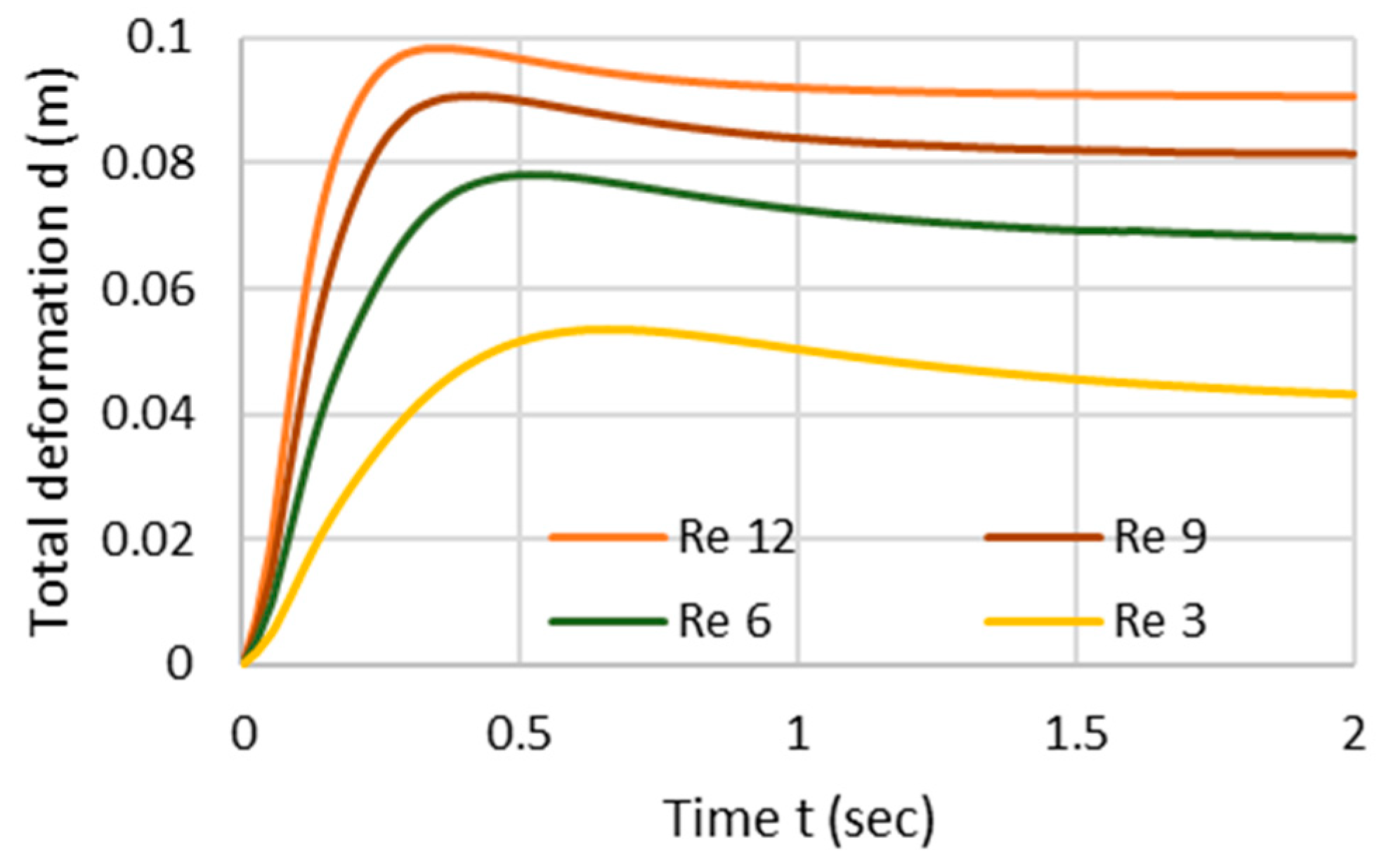
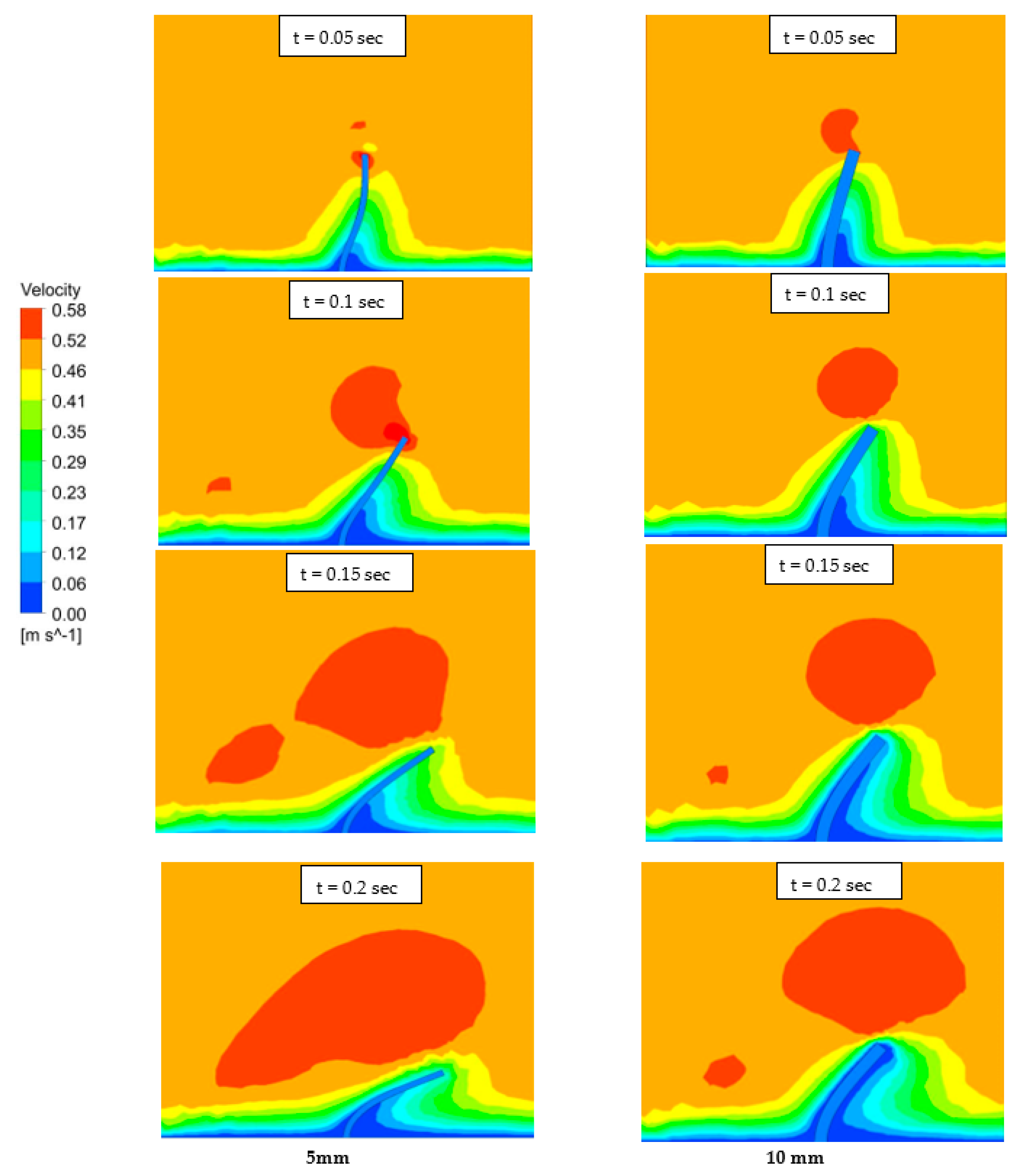
The present investigation focuses on the numerical investigation of flexible flaps in a glycerin environment for different thicknesses and flap orientations. The deformation of the flaps was measured to observe the various flap clamping positions under laminar flow and also the maximum tip-deflection of the flap was observed. For both experimental and simulation conditions, the flaps settle down to a steady-state and the bending patterns attained by current simulation model are very close to that observed in the experiments. The focus of the present FSI simulations is to design a 3D interaction between structure and fluid in order to narrow the literature gap for flexible structures. The results indicate that flap bending increases with the increase in Reynolds number in the range of 3 < Re < 12. However, for a different clamping position of 0° to 90° indicates minimum flap deflection with the highest clamping angle. Correspondingly, for an inclined position of 45° less deflection is perceived as compared to its undeformed shape. The objective is to judge the flap positions and flow regimes at varying computational time and to observe transient deformation response under different flow velocities. Likewise, the drag coefficients are also predicted for various flap alignments. Henceforward, the numerical model is suitable to accurately predict the response of thick and relatively thinner structures.

The flap bending in the current work is observed for low Reynolds number; however, the bending and periodic nature of flap motion is schedule by another 3D FSI model for higher Reynolds number in case of water as a working fluid. For this purpose, experiments will be performed for thinner flaps and the numerical model will be helpful in understanding the flow physics around the flaps. This will be further helpful in designing the flexible structures in hemodynamic, biomedical and structural dynamics.