Optimal Design of Fuzzy Systems Using Differential Evolution and Harmony Search Algorithms with Dynamic Parameter Adaptation

Abstract

This paper presents a study of two popular metaheuristics, namely differential evolution (DE) and harmony search (HS), including a proposal for the dynamic modification of parameters of each algorithm. The methods are applied to two cases, finding the optimal design of a fuzzy logic system (FLS) applied to the optimal design of a fuzzy controller and to the optimization of mathematical functions. A fuzzy logic controller (FLC) of the Takagi–Sugeno type is used to find the optimal design in the membership functions (MFs) for the stabilization problem of an autonomous mobile robot following a trajectory. A comparative study of the results for two modified metaheuristic algorithms is presented through analysis of results and statistical tests. Results show that, statistically speaking, optimal fuzzy harmony search (OFHS) is better in comparison to optimal fuzzy differential evaluation (OFDE) for the two presented study cases.

1. Introduction

Recently, the harmony search algorithm (HS) has proven to be an interesting method in solving complex problems in intelligent computing, and several authors are focused on implementing this algorithm in different fields on computer science. For example, advances for this algorithm are presented by Kim et al. in [1], HS-based management of distributed energy and storage systems in microgrids is described by Ceylan et al. in [2], an HS is used for neural networks to improve fraud detection in banking system by Daliri in [3], a discrete HS for flexible job shop scheduling problem with multiple objectives is explained by Gao et al. in [4], a HS for optimal design of PID controller is described by Kayabekir et al. in [5], an HS method to solve the vehicle routing problem by Liu et al. in [6], an improved HS is described by Ouyang et al. in [7], an HS with dynamic adaptation of Parameters for problem control presented by Peraza et al. in [8], an HS for feature selection for facial emotion recognition using cosine similarity by Saha et al. in [9], a novel HS and its application to data clustering presented by Talaei et al. in [10], a case study to test a fuzzy HS is described by Valdez et al. in [11], and an improved differential-based HS with linear dynamic domain is presented by Zhu et al. in [12].

Another important meta-heuristic that has proven to be an excellent algorithm based on its implementation results in different areas of intelligent computing is the differential evolution (DE) algorithm, and some important works using DE include an Adaptive DE with novel mutation strategies in multiple sub-populations presented by Cui et al. in [13], a novel DE for solving constrained engineering optimization problems presented by Mohamed in [14], a hybrid real-code population-based incremental learning and DE for many-objective optimization of an automotive floor-frame described by Pholdee et al. in [15], time series forecasting for building energy consumption using weighted support vector regression with DE optimization technique presented by Zhang et al. in [16], an improved adaptive DE for continuous optimization outlined by Yi et al. in [17], and an adaptive DE with sorting crossover rate for continuous optimization problems presented by Zhou et al. in [18].

To validate the efficiency in the performance of the metaheuristics algorithms, two cases are used. The first one is in the area of stabilization of non-linear plants, and the second one is the area of mathematical functions. For the first case, some interesting related works can be mentioned—a Particle Swarm Optimization-Modified Frequency Bat (PSO-MFB) is implemented for stable path planning of an autonomous mobile robot (AMR) as presented by Ajeil et al. [19], the use of multiple sensors for AMR navigation is presented by Hoang et al. [20], a mobile robot path-planning using oppositional-based improved firefly algorithm under cluttered environment is presented by Panda et al. [21], fuzzy sets in dynamic adaptation of parameters of a bee colony optimization for controlling the trajectory of an AMR are presented by Amador-Angulo et al. [22], a robot path planning using modified artificial bee colony algorithm is presented by Nayyar et al. [23], and a design and implementation of a fuzzy path optimization system for omnidirectional AMR in real-time is presented by Cuevas et al. [24]. An interesting work where DE is used in the field of non-linear plants is for robot path planning as presented by Jain et al. [25]. In this work, the optimal design of the MFs is search for a fuzzy logic system (FLS) [26,27], specifically a Takagi–Sugeno fuzzy controller is used in the experiments, this inference mechanisms in the FLS is an excellent tool a comparative of fuzzy sets, for example; a Takagi–Sugeno fuzzy logic controller (FLC) for a Liu–Chen four-scroll chaotic system is presented by Vaidyanathan et al. in [28], a Whale optimization algorithm-based Sugeno FLC for fault ride-through improvement of grid-connected variable speed wind generators is presented by Qais et al. in [29], a Fault tolerant trajectory tracking control design for interval-type-2 Takagi-Sugeno fuzzy logic system is outlined by Maalej et al. in [30], a Sugeno–Mamdani fuzzy system based soft computing approach toward sensor node localization with optimization is presented by Kumar et al. in [31], a hybrid technique of Mamdani and Sugeno–based fuzzy interference system approach is explained by Devi et al. in [32], an optimization of fuzzy logic (Takagi–Sugeno) blade pitch angle controller in wind turbines by genetic algorithm is presented by Civelek in [33], a control and balancing of two-wheeled mobile robots using Sugeno fuzzy logic in the domain of AI techniques is presented by Chouhan et al. in [34], and a stable Takagi–Sugeno fuzzy control designed by optimization is presented by Vrkalovic et al. in [35].

The second important field in intelligent computing to evaluate metaheuristic algorithms is in mathematical functions, and some interesting related works include Hussien et al. presenting a New binary whale optimization algorithm for discrete optimization problems [36]; Ochoa et al. presenting a DE with a fuzzy logic approach for dynamic parameter adjustment using benchmark functions [37]; Peraza et al. presenting an HS with dynamic adaptation of parameters for the optimization of a benchmark set of functions [38]; Rao presents the Rao algorithms—three metaphor-less simple algorithms for solving optimization problems [39]; Sulaiman et al. presenting a barnacles mating optimizer—a new bio-inspired algorithm for solving engineering optimization problems [40]; Yue et al. presenting a hybrid grasshopper optimization algorithm with invasive weed for global optimization [41]; and Perez et al. presenting a bat algorithm comparison with genetic algorithm using benchmark functions [42]. Finally, an interesting work is presented by Mulo et al. as a combination of modified HS and DE optimization techniques in economic load dispatch [43].

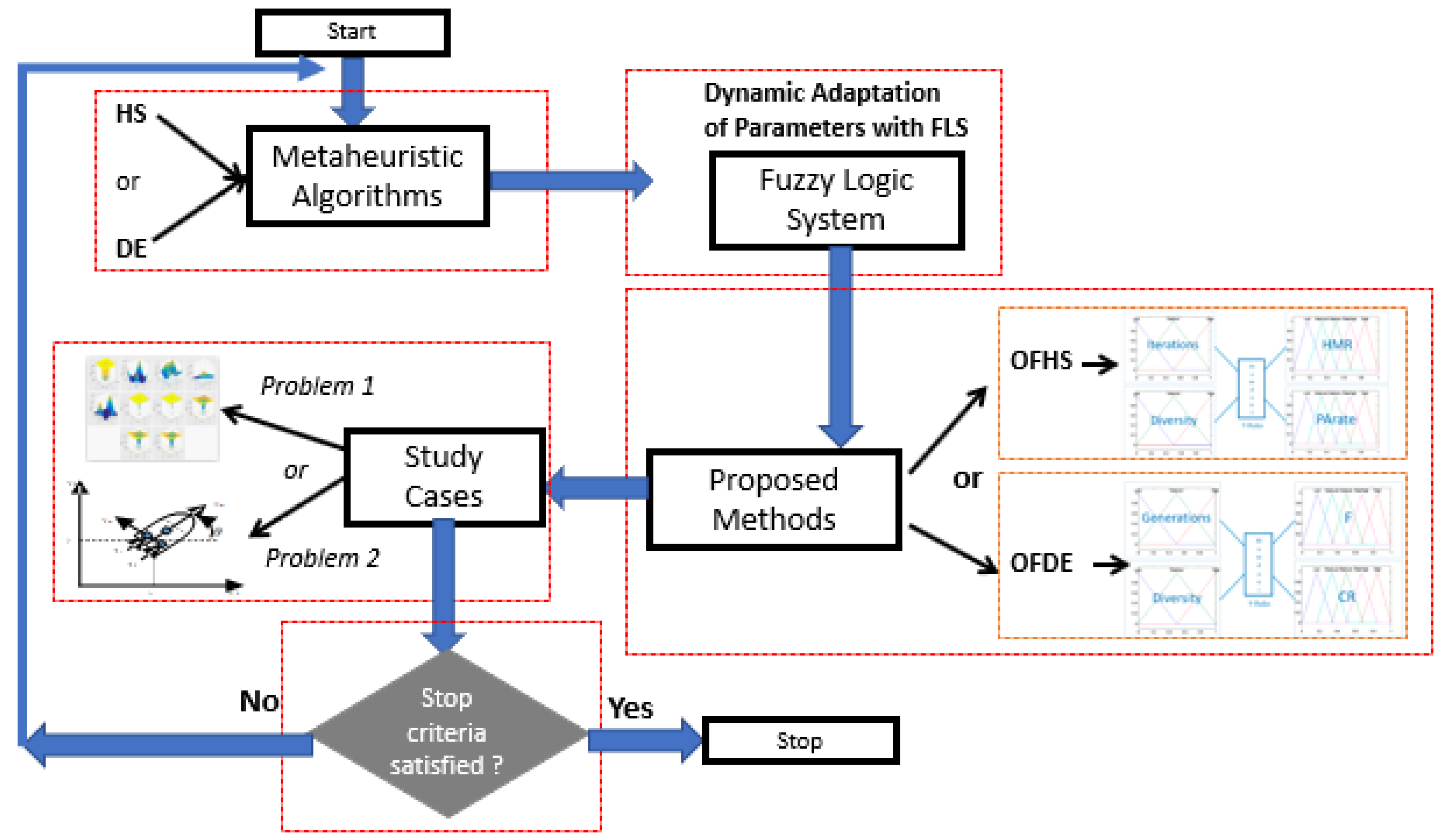
Therefore, it is important to analyze the study cases that have been implemented in the works previously presented [37,38]. In this paper, two metaheuristic algorithms are implemented, which are harmony search (HS) and differential evolutional (DE); the main purpose is to find the optimal parameters for each algorithm that allows the user to minimize the fitness functions in each of the study cases. Thus, an improvement on the original algorithm is proposed with the dynamic adaptation of parameters through the fuzzy logic system, specially to find the optimal design in the values for HS for harmony memory accepting (HMR) and pitch adjustment rate (PArate) to represent the optimized fuzzy harmony search (OFHS) and the dynamic parameters for mutation rate (F) and crossover rate (CR) for DE to represent the optimized fuzzy differential evolution (OFDE). The two proposed methods are applied for optimizing fuzzy controllers and mathematical functions, a statistical test is presented with the obtained results, and the main objective is to measure the efficiency in the performance of metaheuristic algorithms for the two study cases.

The organization of the sections in this paper is described in the following. Section 2 describes two metaheuristics implemented in this paper; Differential Evolution and Harmony Search Algorithms, Section 3 describes the optimal design of fuzzy system approach for the two study cases. Section 4 describes two study cases to analyze—the first is the stabilization of trajectory for an autonomous mobile robot (AMR), and the second is the optimization in mathematical functions. Section 5 describes a comparative of the results for the metaheuristic algorithms, and a statistical test is also presented. Section 6 presents some relevant conclusions and future works for this paper.

2. Meta-Heuristic Background

Metaheuristics are used for problem solving. This section describes the basic concepts of two metaheuristics that are used later in the paper, which have had great impact on the solution of different problems and are presented in more detail in the following subsections.

2.1. Differential Evolution Algorithm

In 1994, Storn and Price proposed the differential evolution (DE) algorithm [44], and the basic structure of the algorithm is based mainly on the following operations:

2.1.1. Population Structure

The DE contains Np D-dimensional vectors of real-valued parameters, where $P_x:Thecurrentpopulation,x_{i,g}$: is composed of those vectors, and indices start with 0 to simplify working with arrays and modular arithmetic. The index, $g=0,1,\dots , g_{max}$, indicates the generation to which a vector belongs. Once initialized, DE mutates randomly chosen vectors to produce an intermediary population $P_{v,g}$ of $Np$ mutant vectors, $v_{i,g}$. Each vector in the current population is recombined with a mutant vector to produce a trial population, P_u, the NP, mutant vector $u_{i,g}$.

$$P_{x,g}=\left(x_{i,g}\right), i=0,1,\dots , Np-1, g=0,1,\dots , g_{max}$$

(1)

$$x_{i,g}=\left(x_{j,i,g}\right), j=0,1,\dots ,D-1$$

(2)

$$P_{v,g}= \left(v_{i,g}\right), i=0,1,\dots , Np-1, g=0,1,\dots , g_{max}$$

(3)

$$v_{i,g}=\left(v_{j,i,g}\right), j=0,1,\dots ,D-1$$

(4)

$$P_{u,g}= \left(u_{i,g}\right), i=0,1,\dots , Np-1, g=0,1,\dots , g_{max}$$

(5)

$$u_{i,g}=\left(u_{j,i,g}\right), j=0,1,\dots ,D-1$$

(6)

2.1.2. Initialization

The upper and lower limits of each parameter must be established, and these 2D values can be collected by two initialized vectors—D-dimensional, $b_L$ y $b_U$, where the subscripts L and U indicate the lower and upper limits, respectively.

$$x_{j,i,0}=ran{d}_j\left(0,1\right)\times \left(b_{j,U}-b_{j,L}\right)+ b_{j,L}$$

(7)

2.1.3. Mutation

Three vectors are selected at random which multiplied by a scale factor F create the mutated vector, the scale factor, F ∈ (0, 1) is a positive real number that controls the rate at which the population evolves.

$$v_{i,g}= x_{r_0,g}+\mathrm{F}\times \left(x_{r_1,g}-x_{r_2,g}\right)$$

(8)

2.1.4. Crossover

A uniform crossover, also known as discrete (dual) recombination is used to search for differential mutations, where Cr ∈ (0, 1) is a positive real number:

$$u_{i,g}= u_{j,i,g}\{\begin{array}{c}{v}_{j,i,g} if \left(ran{d}_j\left(0,1\right)\le Cr or j=j_{rand}\right)\\ x_{j,i,g otherwise}\end{array}$$

(9)

2.1.5. Selection

In this operation, the test vector is analyzed,$u_{i,g},$ in case it has a value equal to or less than its target vector,$x_{i,g}.$ The target vector is replaced in the next generation, otherwise the target retains its place in the population until the condition is met:

$$x_{i,g+1}= \{\begin{array}{c}{u}_{i,g} if f\left(u_{i,g}\right)\le f\left(x_{i,g}\right)\\ x_{i,g} otherwise\end{array}$$

(10)

The aforementioned operations are repeated until the stopping criterion is satisfied.

2.2. Harmony Search Algorithm

Harmony search (HS) was originally proposed by Zong Woo Geem in 2001 [45]. This algorithm is inspired by jazz music composition. It is made up of the following five operations:

Step 1: Initialize the problem and parameters, LB and UB indicate the lower and upper limits, respectively:

$$\mathrm{Minimize}f\left(x\right)s.t. x\left(j\right)\in [LB\left(j\right), UB\left(j\right)\}, j=1,2,\dots , n].$$

(11)

Step 2: Initialize the harmony memory (HM):

$$HM=\left[\begin{array}{ccccc}{x}_1^1& x_2^1& \dots & x_N^1& f\left(x^1\right)\\ x_1^2& x_2^2& \dots & x_N^2& f\left(x^2\right)\\ ⋮& ⋮& ⋮& ⋮& ⋮\\ x_1^{HMS}& x_2^{HMS}& \dots & x_N^{HMS}& f\left(x^{HMS}\right)\end{array}\right]$$

(12)

Step 3: Improvise a new harmony: improvisation is the most important part of the algorithm because the memory considerations (HMR), pitch adjustment (PAR), and randomization operations are generated, as indicated in the following equation:

$$X_{new}\left(j\right)=X_{new}\left(j\right)\pm r \times BW$$

(13)

Step 4: Update the harmony memory: the objective function is used to evaluate the HM update with a new solution vector x_ (new). It is compared if the new vector solution is better than the worst solution of the historical vector, and then the worst historical solution is excluded and replaced by a new one.

Step 5: Check the stopping criteria: the aforementioned operations are repeated until the stop criterion is satisfied.

3. Optimal Design of Fuzzy Systems Approach

The proposed method is based on the concepts and equations of the original DE and HS algorithms. Both original algorithms have the problem of parameters being fixed throughout the iterations. In previous work, this problem was eliminated using fuzzy logic to perform the dynamic parameter adjustment. This method consisted of a Mamdani fuzzy system with two inputs (iterations and diversity) and two outputs for each method, as shown by Castillo et al. in [46].

Therefore, the main contribution in this paper is that the proposed method uses the original DE and HS algorithms to find the best architecture of the previous fuzzy differential evolution (FDE) and fuzzy harmony search (FHS) fuzzy systems shown by Castillo et al. in [46], which are responsible for adjusting parameters along the iterations. The proposed methods are optimized fuzzy differential evolution (OFDE) and optimized fuzzy harmony search algorithm (OFHS). Once the best architectures of the proposed OFDE and OFHS algorithms have been found, two types of problems are considered for optimization: benchmark mathematical functions and a non-linear control problem. Figure 1 shows the general diagram of the proposed method in this paper.

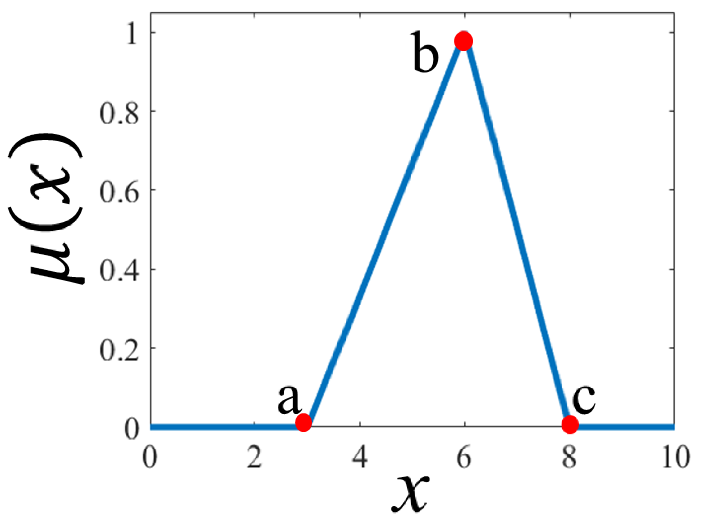
The proposed fuzzy systems have triangular membership functions at the inputs and outputs in both algorithms. The triangular membership function depends on three parameters which are a, b, and c as given by Equation (14), where a and c represents the lower parts of the triangle and b locates the peak. This triangular membership function is represented graphically in Figure 2.

$$f\left(x;a, b,c\right)=max\left(\min \left(\frac{x-a}{b-a},\frac{c-x}{c-b}\right),0\right)$$

(14)

Table 1. Mathematical representation of the input membership functions.

$\mathrm{Low}$	$\mathsf{\mu }\mathrm{Low}\left(\mathrm{x}\right)=\max \left(\min \left(\frac{\mathrm{x}-0.5}{0-0.5},\frac{0.5-\mathrm{x}}{0.5-0}\right),0\right)$
$\mathrm{Medium}$	$\mathsf{\mu }\mathrm{Medium}\left(\mathrm{x}\right)=\max \left(\min \left(\frac{\mathrm{x}-0}{0.5-0},\frac{1-\mathrm{x}}{1-0.5}\right),0\right)$
$\mathrm{High}$	$\mathsf{\mu }\mathrm{High}\left(\mathrm{x}\right)=\max \left(\min \left(\frac{\mathrm{x}-0.5}{1-0.5},\frac{1.5-\mathrm{x}}{1.5-1}\right),0\right)$

and

Table 2. Mathematical representation of the output membership functions.

$\mathrm{Low}.$	$\mathsf{\mu }\mathrm{Low}\left(\mathrm{x}\right)=\max \left(\min \left(\frac{\mathrm{x}-0.005}{0.17-0.005},\frac{0.3-\mathrm{x}}{0.3-0.17}\right),0\right)$
$\mathrm{Medium}$ Low	$\mathsf{\mu }\mathrm{Medium}\mathrm{Low}\left(\mathrm{x}\right)=\max \left(\min \left(\frac{\mathrm{x}-0.17}{0.3-0},\frac{1-\mathrm{x}}{1-0.5}\right),0\right)$
$\mathrm{Medium}$	$\mathsf{\mu }\mathrm{Medium}\left(\mathrm{x}\right)=\max \left(\min \left(\frac{\mathrm{x}-0.3}{0.5-0.3},\frac{0.7-\mathrm{x}}{0.7-0.5}\right),0\right)$
Medium High	$\mathsf{\mu }\mathrm{Medium}\mathrm{High}\left(\mathrm{x}\right)=\max \left(\min \left(\frac{\mathrm{x}-0.5}{0.5-0.7},\frac{0.85-\mathrm{x}}{0.85-0.7}\right),0\right)$
High	$\mathsf{\mu }\mathrm{High}\left(\mathrm{x}\right)=\max \left(\min \left(\frac{\mathrm{x}-0.7}{0.85-0.7},\frac{1-\mathrm{x}}{1-0.85}\right),0\right)$

summarize the representation of the knowledge of the inputs and outputs of the fuzzy system with triangular membership functions.

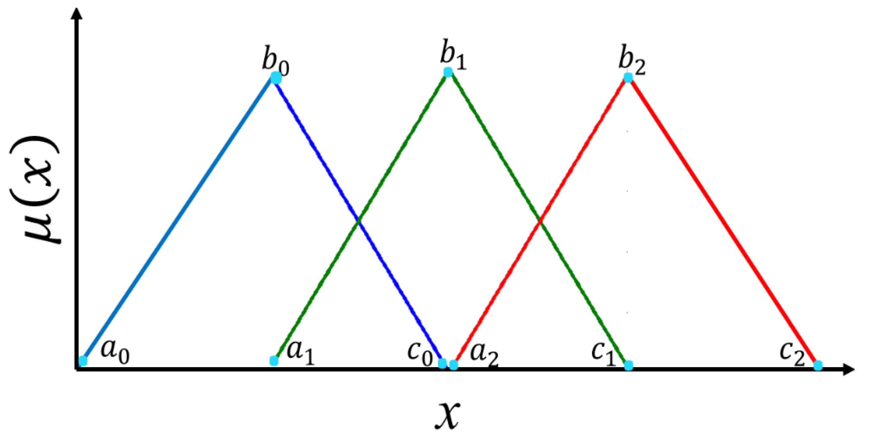
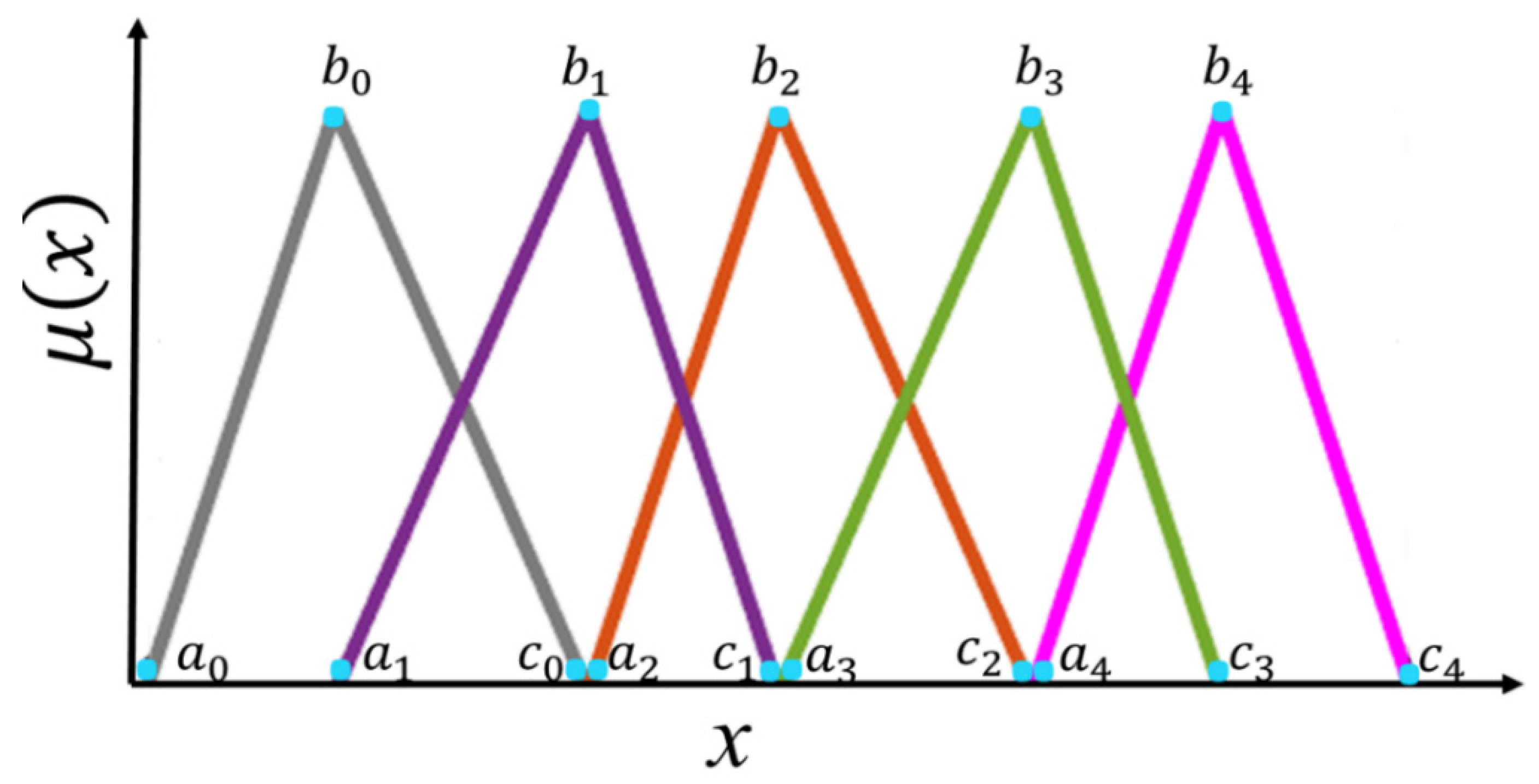
Figure 3 and Figure 4 illustrate the parameters that form each input and output triangular membership function.

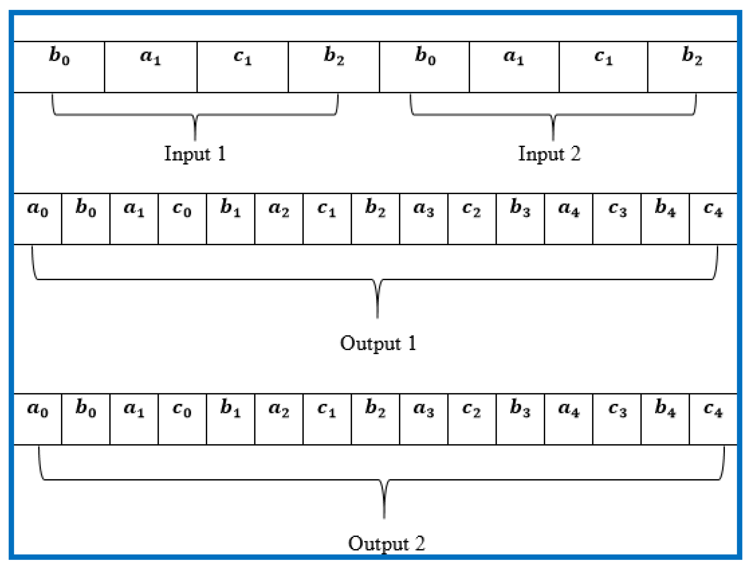
The fuzzy system was optimized with DE and HS; in the DE, it is necessary to use a chromosome, and in HS, a harmony to optimize the membership functions (MFS) is necessary, and in this case, it is called a vector, as shown in Figure 5. The vector has 44 positions, of which six parameters are fixed and 38 are optimized.

The limits for the optimization of each triangular membership function are specified in

Table 3. Limits of the parameters of the membership functions.

	Input 1	Input 2	Output 1	Output 2
MFs Parameters	Low MF: $a_0=0$ $0\le b_0\le 0.5$ $c_0=0.5$	Low MF: $a_0=0$ $0\le b_0\le 0.5$ $c_0=0.5$	Low MF: $0\le a_0\le 0.17$ $b_0=0.17$ $0.17\le c_0\le 0.35$	Low MF: $0\le a_0\le 0.17$ $b_0=0.17$ $0.17\le c_0\le 0.35$
	Medium MF: $0\le a_1\le 0.5$ $b_1=0.5$ $0.5\le c_1\le 1$	Medium MF: $0\le a_1\le 0.5$ $b_1=0.5$ $0.5\le c_1\le 1$	Medium Low MF: $0.17\le a_1\le 0.35$ $b_1=0.35$ $0.35\le c_1\le 0.5$	Medium Low MF: $0.17\le a_1\le 0.35$ $b_1=0.35$ $0.35\le c_1\le 0.5$
	High MF: $a_2=0.5$ $0.5\le b_2\le 1$ $c_2=1$	High MF: $a_2=0.5$ $0.5\le b_2\le 1$ $c_2=1$	Medium MF: $0.35\le a_2\le 0.5$ $b_2=0.5$ $0.5\le c_2\le 0.7$	Medium MF: $0.35\le a_2\le 0.5$ $b_2=0.5$ $0.5\le c_2\le 0.7$
	-	-	Medium High MF: $0.5\le a_3\le 0.7$ $b_3=0.7$ $0.7\le c_3\le 0.85$	Medium High MF: $0.5\le a_3\le 0.7$ $b_3=0.7$ $0.7\le c_3\le 0.85$
	-	-	High MF: $0.7\le a_4\le 0.85$ $b_4=0.85$ $0.85\le c_4\le 1$	High MF: $0.7\le a_4\le 0.85$ $b_4=0.85$ $0.85\le c_4\le 1$

.

4. Study Cases

Two types of problems are used in this work in order to validate the proposed methodology. The first one is benchmark mathematical functions, and the second one is a benchmark control problem of the Sugeno type. The explanation of each of the problems is shown in more detail in the following subsections.

4.1. Benchmark Mathematical Functions

A set of eight benchmark mathematical functions are selected for the first part of the experimentation. The idea of using mathematical functions is to explore the behavior of our proposal. In

Table 4. Benchmark mathematical functions.

Function	Search Domain	F Min	Equation
Rosenbrock	[−5, 10] n	0	$f\left(x\right)={\displaystyle \sum _{i=1}^{n-1}}\left[100{\left(x_{i-1}-x_i^2\right)}^2+{\left(1-x_1\right)}^2\right]$
Sphere	[−5.12, 5.12] n	0	$f\left(x\right)={\displaystyle \sum _{i=1}^n}{x}_i^2$
Rastrigin	[−5.12, 5.12] n	0	$f\left(x\right)=10n+{\displaystyle \sum _{i=1}^n}\left[x_i^2-10cos\left(2x_i\right)\right]$
Schwefel	[−500, 500] n	0	$f\left(x\right)={\displaystyle \sum _{i=1}^n}\left[-x_{i}sin\left(\sqrt{\left|x_i\right|}\right)\right]$
Sum squares	[−10, 10] n	0	$f\left(x\right)={\displaystyle \sum _{i=1}^n}i{x}_i^2$
Zakharov	[−5, 10] n	0	$f\left(x\right)={\displaystyle \sum _{i=1}^n}{x}_i^2+{({\displaystyle \sum _{i+1}^n}0.5i{x}_i)}^2+{({\displaystyle \sum _{i=1}^n}0.5i{x}_i)}^4$
Griewank	[−600, 600] n	0	$f\left(x\right)=\frac{1}{400} {\displaystyle \sum _{i=1}^n}{X}_i^2-{\displaystyle \prod _{i=1}^n}cos\left(\frac{x_i}{\sqrt{i}}\right)+1$
Powell	[−4, 5] n	0	$f\left(x\right)={\displaystyle \sum }_{i=1}^{n/4}[{(x_{4i-3}+10x_{4i-2})}^2+5{(x_{4i-1}- x_{4i})}^2+{(x_{4i-2}- 2x_{4i-1})}^4+$10($x_{4i-3}- x_{4i}{)}^4]$

we show the search domain, minimum and their respective equation for each benchmark function.

The set of used functions is diverse, as we have simple functions and at the same time complicated functions, including both levels of complexity helps in our experimentation to check that it works in simple functions, as well as in complicated functions.

4.2. Robot Mobile Controller

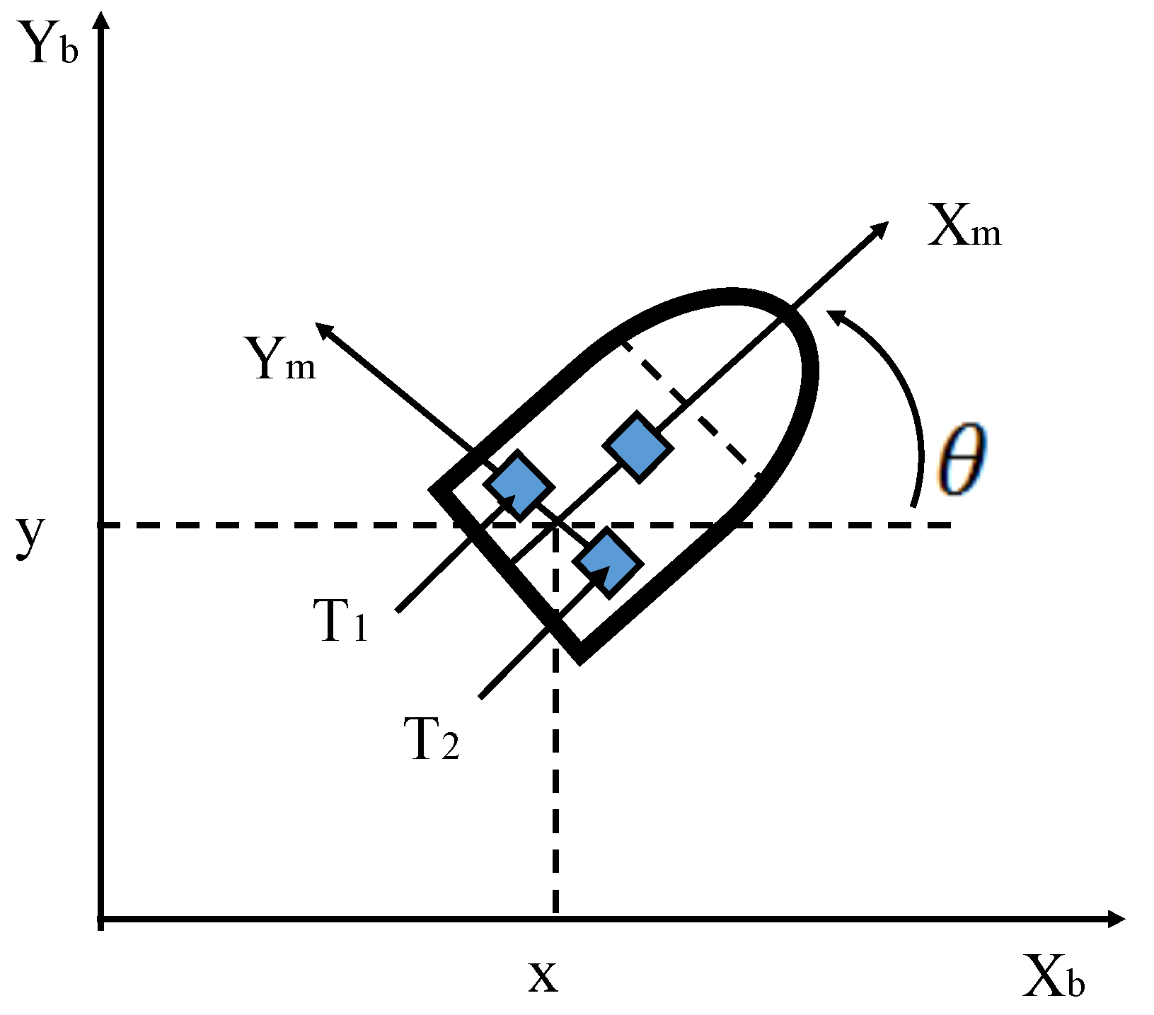
The second control problem is a unicycle mobile robot, and a Sugeno type controller was used, which has a higher level of complexity. The main goal of this controller is to make the robot follow a reference trajectory. The robot is composed of two drive wheels located on the same axis and a front free wheel that is used only for stability. The graphical representation of the robot mobile is illustrated in Figure 6, in which we can observe the two wheels that make up the robot, the two torques, and the angle with respect to the Y axis.

Equations (15) and (16) represent the operation of the mathematical model of the mobile robot, and for each equation a brief explanation is given of each of the variables that constitute the equations is presented.

$$M\left(q\right)\dot{v}+C\left(q,\dot{q}\right)v+Dv= \mathsf{\tau }+\mathrm{P}\left(\mathrm{t}\right)$$

(15)

where

$\mathrm{q}={\left(\mathrm{x},\mathrm{y},\mathsf{\theta }\right)}^{\mathrm{T}}$ is the vector of the configuration coordinates;

$\mathrm{v}={\left(\mathrm{v},\right)}^{\mathrm{T}}$ is the vector of velocities;

$\mathsf{\tau }=\left({\mathsf{\tau }}_{1,}{\mathsf{\tau }}_2\right)$ is the vector of torques applied to the wheels of the robot where ${\tau }_1$ and ${\tau }_2$ denote the torques of the right and left wheel, respectively;

$P\in R^2$ is the uniformly bounded disturbance vector;

$M\left(q\right)\in R^{2X2}$ is the positive-definite inertia matrix;

$C\left(q,\dot{q}\right)\vartheta$ is the vector of centripetal and Coriolis forces;

$D \in R^{2X2}$ is a diagonal positive-definite damping matrix.

The kinematic system is determined by Equation (16):

$$\dot{q}=\left[\begin{array}{cc}\cos \theta & 0\\ \sin \theta & 0\\ 0& 1\end{array}\right]\left[\begin{array}{c}v\\ \omega \end{array}\right]$$

(16)

where

(x,y) is the position in the $X-Y$ (world) reference frame;

$\theta$ is the angle between the heading direction and the x-axis;

$v and \omega$ are the linear and angular velocities, respectively.

Equation (17) represents the non-holonomic constraint, which this system has, which corresponds to a non-slip wheel condition preventing the robot from moving sideways.

$$\dot{y }\cos \theta -\dot{x}\sin \theta =0$$

(17)

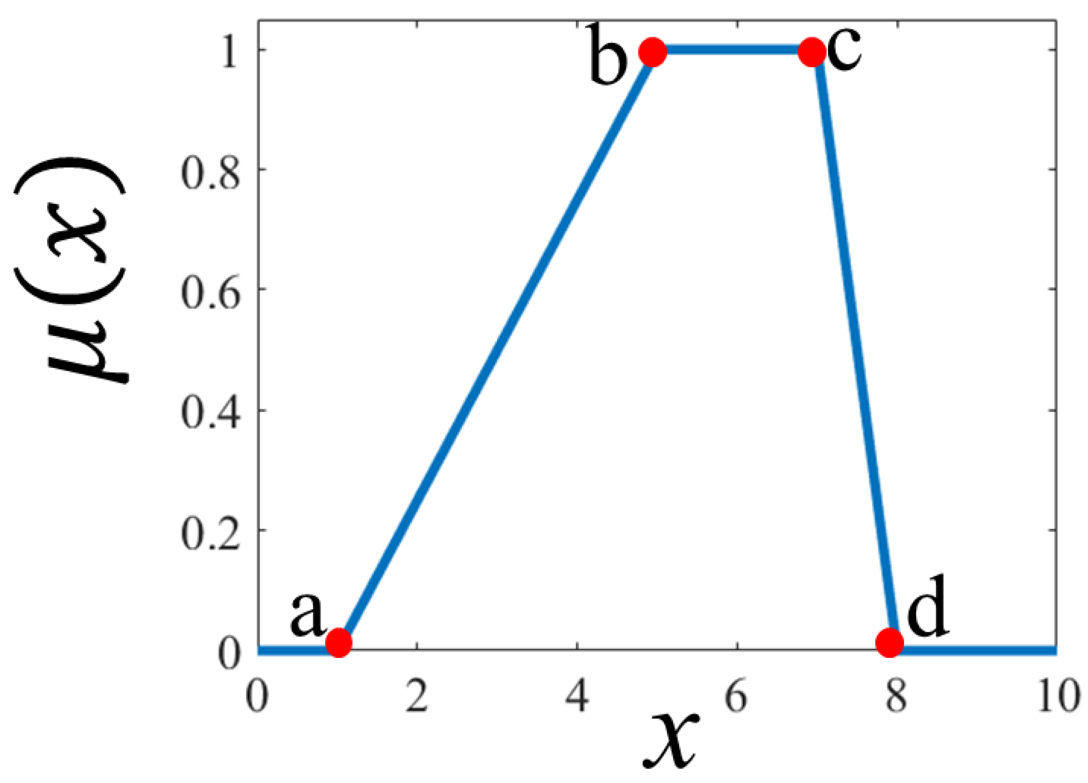
One of the membership functions used in the controller is the trapezoidal one, which has four scalar parameters—a, b, c, and d as given by the Equation (18), where a and d represents the lower corners of the trapezoid and the b and c locate the shoulders. To represent the graphical form of the trapezoidal membership function, we illustrate it in Figure 7.

$$f\left(x;a, b,c,d\right)=max\left(\min \left(\frac{x-a}{b-a},1,\frac{d-x}{d-c}\right),0\right)$$

(18)

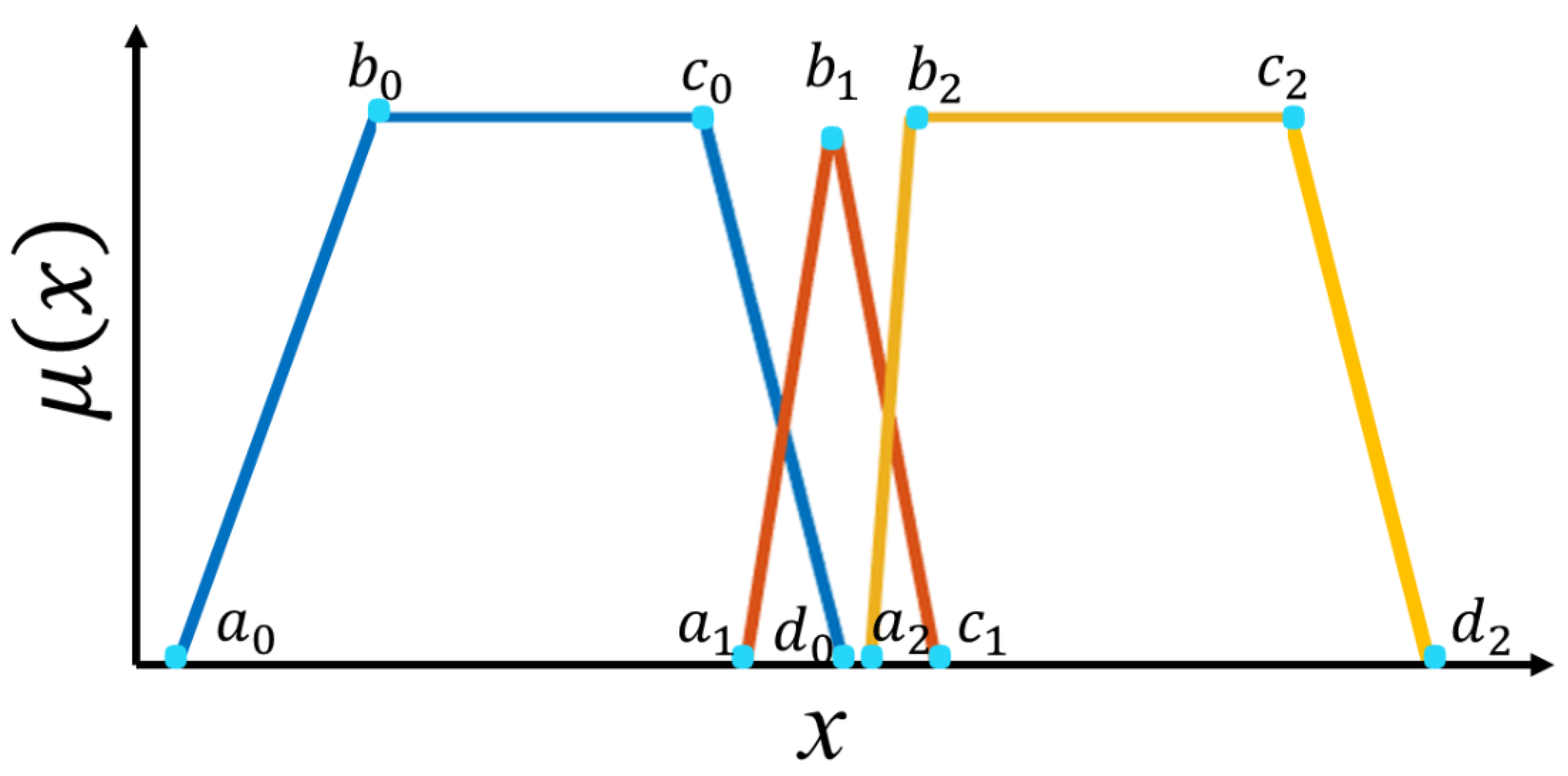
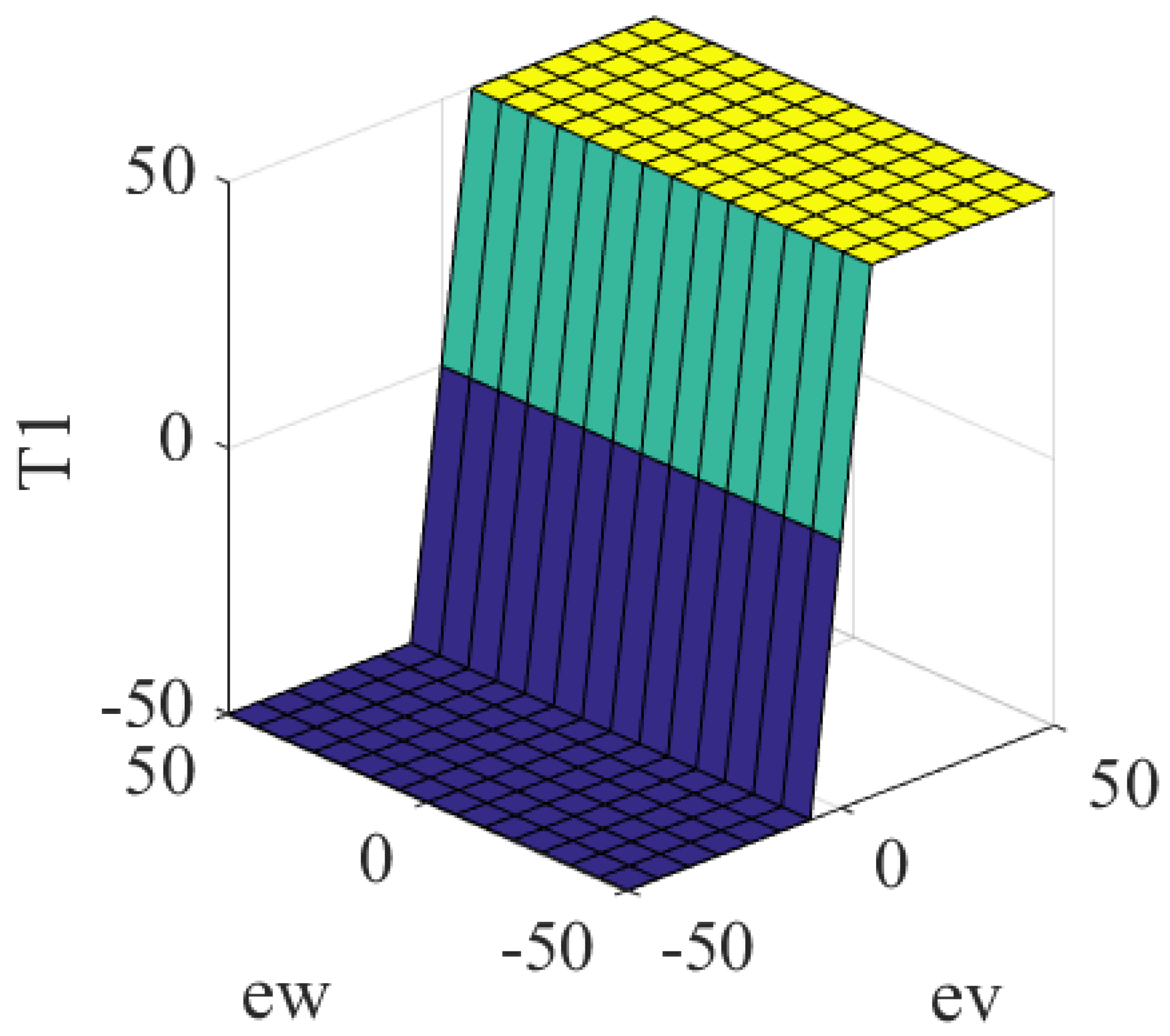
The structure of the fuzzy system of the Sugeno-type controller is composed of two inputs: the first one is the linear velocity error, and the second is the angular velocity error, which are granulated into three membership functions (negative, zero, positive). Both are composed of trapezoidal functions on the extremes and a triangular one in the center, as can be appreciated in Figure 8.

Table 5. Mathematical representation of the input 1 membership function.

Linear Velocity Error (ev)
Negative (N)	$\mathsf{\mu }\mathrm{N}\left(\mathrm{x}\right)=\max \left(\min \left(\frac{\mathrm{x}+50}{-50+50},1,\frac{-1-\mathrm{x}}{-1+15}\right),0\right)$
Zero (Z)	$\mathsf{\mu }\mathrm{Z}\left(\mathrm{x}\right)=\max \left(\min \left(\frac{\mathrm{x}+4}{0+4},\frac{6-\mathrm{x}}{6-0}\right),0\right)$
Positive (P)	$\mathsf{\mu }\mathrm{P}\left(\mathrm{x}\right)=\max \left(\min \left(\frac{\mathrm{x}-1}{5-1},1,\frac{50-\mathrm{x}}{50-50}\right),0\right)$

and

Table 6. Mathematical representation of the input 2 membership function.

Angular Velocity Error (ew)
Negative (N)	$\mathsf{\mu }\mathrm{N}\left(\mathrm{x}\right)=\max \left(\min \left(\frac{\mathrm{x}+50}{-50+50},1,\frac{-1-\mathrm{x}}{-1+5}\right),0\right)$
Zero (Z)	$\mathsf{\mu }\mathrm{Z}\left(\mathrm{x}\right)=\max \left(\min \left(\frac{\mathrm{x}+2}{0+2},\frac{3-\mathrm{x}}{3-0}\right),0\right)$
Positive (P)	$\mathsf{\mu }\mathrm{P}\left(\mathrm{x}\right)=\max \left(\min \left(\frac{\mathrm{x}-1}{5-1},1,\frac{50-\mathrm{x}}{50-50}\right),0\right)$

show the mathematical knowledge of each membership function for each of the inputs.

The controller used is of the Takagi–Sugeno type and is formed by nine fuzzy rules that govern the trajectory of the robot based on the controller.

Table 7. Rules for the fuzzy logic controller.

ev (Input1)	ew (Input2)	${\mathit{\tau }}_1 \left(\mathbf{O}\mathbf{u}\mathbf{t}\mathbf{p}\mathbf{u}\mathbf{t}1\right)$	${\mathit{\tau }}_2 \left(\mathbf{O}\mathbf{u}\mathbf{t}\mathbf{p}\mathbf{u}\mathbf{t}2\right)$
N	N	N	N
N	Z	N	Z
N	P	N	P
Z	N	Z	N
Z	Z	Z	Z
Z	P	Z	P
P	N	P	N
P	Z	P	Z
P	P	P	P

contains more detail of these fuzzy rules. The Sugeno coefficients of this controller are presented in

Table 8. Sugeno coefficients.

	Negative	Zero	Positive
Torque 1 (${\tau }_1)$	−50	0	50
Torque 2 (${\tau }_2)$	−50	0	50

.

The surface of this controller is shown in detail in Figure 9.

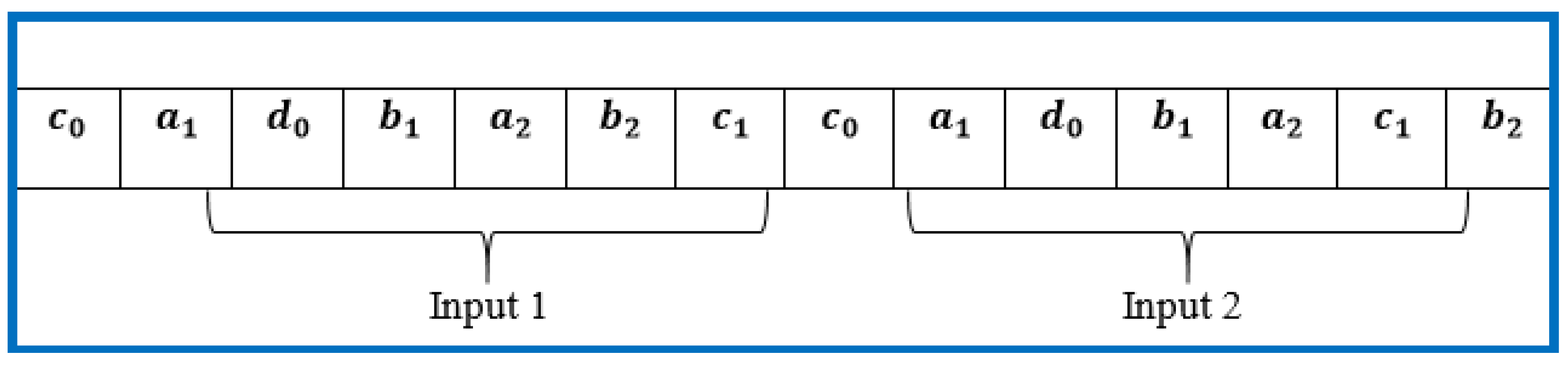
The proposed OFDE and OFHS methods are used to optimize the parameter values of the membership functions of the mobile robot controller in order to minimize the root mean square error (RMSE) described in Equation (19). Figure 10 represents the vector with the points of the membership functions of both controller inputs. It has 22 total points, where eight are fixed and 14 are optimized. These points that we call optimized are the points (parameter values) that the original algorithm provides in order to create a new structure of the fuzzy system.

$$RMSE= \sqrt{\frac{1}{N}{\displaystyle \sum }_{t=1}^N{(x_t-{\widehat{x}}_t)}^2}$$

(19)

The limits for the optimization of each membership function are specified in

Table 9. Limits of the parameters of the membership functions.

	Input 1	Input 2
MFs Parameters	Negative MF: $a_0=b_0=-50$ $-50<c_0<-15$ $-15<d_0<-1$	Negative MF: $a_0=b_0=-50$ $-50<c_0<-5$ $-5<d_0<-1$
	Zero MF: $-50<a_1<0$ $b_1=0$ $0<c_1<50$	Zero MF: $-50<a_1<0$ $b_1=0$ $0<c_1<50$
	Positive MF: $-1<a_2<5$ $0<b_2<50$ $c_2=d_2=50$	Positive MF: $-1<a_2<5$ $0<b_2<50$ $c_2=d_2=50$

.

5. Comparison of Results

Experiments were performed with the proposed OFDE and OFHS algorithms applied to benchmark mathematical functions and benchmark control cases to validate the proposed methodology. This section shows the experimentation and the obtained results.

5.1. Results for the Benchmark Mathematical Functions

Thirty experiments were performed with the proposed OFDE and OFHS methods applied to each of the eight benchmark mathematical functions shown in Section 4.1. The simulations were obtained as a result of software implemented in Matlab 2013 and 2015, from Mathworks, Los Angeles, CA, USA. The parameters used for the experiment for the OFDE method are shown in

Table 10. Parameters used in the experiment for the OFDE method.

Parameters	OFDE
Population	150
Dimension	50
Generation	2000
Run	30
F	Dynamic
CR	Dynamic

and for the OFHS method are presented in

Table 11. Parameters used in the experiment for the OFHS method.

Parameters	OFDE
Harmony	150
Dimension	50
Iteration	2000
Run	30
HMR	Dynamic
PArate	Dynamic

.

Table 10 shows the values of the population, dimension, generation, run, mutation rate (F), and crossover rate (CR) parameters used in the experiment for the proposed OFDE.

Table 11 shows the values of the harmony, dimension, iteration, run, harmony memory accepting (HMR), and pitch adjustment rate (PArate) parameters used in the experiment for the proposed OFHS.

The results obtained by using the proposed OFDE method are shown in

Table 12. Results of the OFDE method applied to benchmark mathematical functions.

Function	Minimum	Maximum	Average	Std	Execution Time
Sum Square	7.60 × 10−24	1.05 × 10−4	4.12 × 10−6	1.93 × 10−5	20,467.8 s
Rosenbrock	3.56 × 10−18	3.20 × 10−7	8.20 × 10−8	1.20 × 10−7	22,851.6 s
Sphere	1.20 × 10−7	2.55 × 10−22	8.49 × 10−24	4.65 × 10−23	15,782.6 s
Rastrigin	5.10 × 101	1.31 × 102	9.67 × 101	1.74 × 101	21,979.2 s
Schwefel	3.82 × 10−4	4.69 × 103	1.52 × 103	1.75 × 103	17,696.6 s
Zakharov	4.75 × 10−1	2.49 × 101	7.07 × 100	6.33 × 100	17,468.2 s
Griewank	0.00 × 100	1.85 × 10−4	6.95 × 10−6	3.37 × 10−5	4375.4 s
Powell	3.34 × 10−5	9.19 × 10−3	6.34 × 10−4	1.66 × 10−3	16,920.3 s

, and the results obtained by using the proposed OFHS method are shown in

Table 13. Results of the OFHS method applied to benchmark mathematical functions.

Function	Minimum	Maximum	Average	Std	Execution Time
Sum Square	0.00 × 100	1.33 × 10−2	4.45 × 10−4	2.44 × 10−3	274.92 s
Rosenbrock	3.84 × 10−3	3.42 × 10−2	1.63 × 10−2	7.44 × 10−3	280.6 s
Sphere	1.88 × 10−4	1.44 × 10−3	7.63 × 10−4	3.63 × 10−4	230.7 s
Rastrigin	2.04 × 10−4	6.55 × 10−4	4.91 × 10−4	1.08 × 10−4	616.78 s
Schwefel	1.98 × 10−6	1.45 × 10−1	1.57 × 10−2	3.24 × 10−2	620.76 s
Zakharov	1.46 × 10−14	2.76 × 10−12	4.76 × 10−13	5.63 × 10−13	250.4 s
Griewank	2.22 × 10−16	2.69 × 10−13	6.65 × 10−14	7.78 × 10−14	271.96 s
Powell	1.07 × 10−3	5.18 × 10−3	2.64 × 10−3	9.10 × 10−4	329.8 s

. These tables indicate the execution time of each mathematical function, where we can note lower times for OFHS.

Table 12 and Table 13 show the minimum and maximum obtained errors, the averages of the 30 experiments, and their standard deviations for all the mathematical functions.

A statistical z-test was performed to validate the efficacy of the proposed methods. The claim is that the OFDE method has achieved lower values compared to the OFHS method. The parameters of the statistical test are as follows: Alpha 0.05, confidence level 95%, sample size is 30 and the critical value is −1,645. where

$$\begin{gathered} {\mu }_1=mean of the OFDE algorithm \\ {\mu }_2=mean of the OFHS algorithm \end{gathered}$$

(20)

The hypotheses would be as follows: $H_o: {\mu }_1\ge$ ${\mu }_2$ and $H_a: {\mu }_1<$ ${\mu }_2 \left(Claim\right).$ We can say that there is enough statistical evidence for all values below the critical value Z or −1.645.

Table 14. Results for the statistical test.

Function	Differential Evolution Algorithm		Harmony Search Algorithm		Z-Test
	Average	Std	Average	Std	Z Value	Evidence
Sum Square	4.12 × 10−6	1.93 × 10−5	4.45 × 10−4	2.44 × 10−3	−0.9896	Not significant
Rosenbrock	8.20 × 10−8	1.20 × 10−7	1.63 × 10−2	7.44 × 10−3	−11.9998	Significant
Sphere	8.49 × 10−24	4.65 × 10−23	7.63 × 10−4	3.63 × 10−4	−11.5127	Significant
Rastrigin	9.67 × 101	1.74 × 101	4.91 × 10−4	1.08 × 10−4	30.4394	Not significant
Schwefel	1.52 × 103	1.75 × 103	1.57 × 10−2	3.24 × 10−2	4.7573	Not significant
Zakharov	7.07 × 100	6.33 × 100	4.76 × 10−13	5.63 × 10−13	6.1175	Not significant
Griewank	6.95 × 10−6	3.37 × 10−5	6.65 × 10−14	7.77 × 10−14	1.1296	Not significant
Powell	6.34 × 10−4	1.66 × 10−3	2.64 × 10−3	9.10 × 10−4	−5.8040	Significant

shows the results of the mean, standard deviation, and the Z-values obtained; in three functions, significant evidence is obtained, and in five, no significant evidence is obtained. We can indicate that the OFDE method is not better than OFHS in these mathematical benchmark functions.

5.2. Experiments and Results for the Benchmark Control Problem

Thirty experiments were performed with the proposed OFDE and OFHS methods applied to mobile robot controller. The parameters used for the experiment with the OFDE method are shown in Table 10 and for the OFHS method are shown in Table 11.

The results obtained by optimizing the parameters of the mobile robot controller, with the OFDE and OFHS methods are presented in

Table 15. Results of the OFDE method applied to robot mobile controller.

Method	DE without Noise FLC	DE with Noise FLC	FDE without Noise FLC	FDE with Noise FLC	OFDE without Noise FLC	OFDE with Noise FLC
Minimum	1.23 × 10−1	1.42 × 10−1	4.28 × 10−3	4.28 × 10−3	2.31 × 10−3	3.95 × 10−4
Maximum	4.57 × 100	5.06 × 100	1.32 × 100	1.05 × 100	1.94 × 100	1.50 × 100
Average	1.08 × 100	1.35 × 100	3.83 × 10−1	2.17 × 10−1	2.50 × 10−1	8.78 × 10−2
Std.	1.14 × 100	1.06 × 100	3.53 × 10−1	2.59 × 10−1	4.02 × 10−1	2.68 × 10−1
Execution time	19,372.6 s	23,489.3 s	37,471.16 s	78,320.8 s	155,640.5 s	179,568.2 s

and

Table 16. Results of the OFHS method applied to benchmark controller.

Method	HS without Noise FLC	HS with Noise FLC	FHS without Noise FLC	FHS with Noise FLC	OFHS without Noise FLC	OFHS with Noise FLC
Minimum	4.72 × 10−2	8.02 × 10−2	9.80 × 10−3	9.00 × 10−4	8.90 × 10−3	2.00 × 10−4
Maximum	2.89 × 101	9.81 × 10−1	2.04 × 100	1.14 × 100	2.18 × 10+0	1.26 × 100
Average	1.50 × 100	3.66 × 10−1	3.77 × 10−1	3.26 × 10−1	3.39 × 10−1	2.37 × 10−1
Std.	5.28 × 100	3.00 × 10−1	4.73 × 10−1	3.22 × 10−1	4.61 × 10−1	3.07 × 10−1
Execution time	2529.2 s	3027.8 s	3789.4 s	4295.4 s	8239.3 s	9765.9 s

, respectively. The noise applied to this controller is 0.5 (Gaussian random number). The execution times of each algorithm are also shown.

We can summarize that, in both optimized algorithms, with our proposal, the improvement on average is observed, and in the same way, we can observe that the best result obtained is by using our new proposal. The comparison between the optimized method with noise and without noise also shows that our proposal improves on problems with uncertainty, and this is observed for both algorithms.

Figure 11 and Figure 12 represent the best simulations obtained with each of the methods; for Figure 11, the OFDE method with the best paths without noise and noise are illustrated, and Figure 12 illustrates the OFHS method with the best paths without noise and with noise.

To corroborate the results from both algorithms,

Table 17. Comparison of results with other metaheuristics.

Method	Minimum	Maximum	Average	Std.	Experiments
Results of GAs optimization FLC Type-1 [47]	4.08 × 10−1	5.70 × 10−1	4.37 × 10−1	5.01 × 10−2	29
Results of GAs optimization FLC Type-2 [47]	3.99 × 10−1	4.11 × 10−1	4.01 × 10−1	3.25 × 10−3	30
Ga optimization T1 [48]	4.08 × 10−1	5.70 × 10−1	4.40 × 10−1	4.89 × 10−2	37
Ga optimization FLC Type-2 [48]	3.99 × 10−1	4.11 × 10−1	4.01 × 10−1	3.40 × 10−3	37
ASRank + CONVCONT [49]	2.90 × 10−4	-	1.31 × 10−2	-	30
S-ACO [49]	9.82 × 10−2	-	1.20 × 10−1	-	30
Resulted gbest PSO optimization FLC Type-1 [50]	1.51 × 10−1	1.90 × 100	2.44 × 10−1	3.79 × 10−1	21
Resulted gbest PSO for optimization del FLC Type-2 [50]	1.60 × 10−1	1.61 × 10−1	1.61 × 10−1	2.56 × 10−4	16
OFDE with noise FLC	3.95 × 10−4	1.50 × 100	8.78 × 10−2	2.68 × 10−1	30
OFHS with noise FLC	2.00 × 10−4	1.26 × 100	2.37 × 10−1	3.07 × 10−1	30

is presented, which includes some results using different algorithms and different ways of optimizing applied to this control problem. Table 17 contains the minimum, maximum, average, standard deviation, and the number of experiments for other metaheuristics that were applied to the same problem.

In order to corroborate all the experimentation carried out with our proposal, three methods are chosen from Table 17 to perform statistical tests, and these methods are the only ones that meet the characteristics to perform a Z test.

The following explains how the statistical tests are applied:

Table 18. Statistical test results for OFDE.

Method	OFDE with Noise FLC	Resulted GAs Optimization FLC Type-2 [47]	GA Optimization Type-1 [48]	GA Optimization FLC Type-2 [48]
Minimum	3.95 × 10−4	3.99 × 10−1	4.08 × 10−1	3.99 × 10−1
Maximum	1.50 × 100	4.11 × 10−1	5.70 × 10−1	4.11 × 10−1
Average	8.78 × 10−2	4.01 × 10−1	4.40 × 10−1	4.01 × 10−1
Std.	2.68 × 10−1	3.25 × 10−3	4.89 × 10−2	3.40 × 10−3
Experiments	30	30	37	37
Z Value		−6.4005	−7.0811	−6.4005
Evidence		Significative	Significative	Significative

shows the OFDE results with noise which represents our ${\mu }_1$ and we perform a statistical test for each of the three methods (GAs optimization FLC Type-2, GA optimization Type-1, and GA optimization FLC Type-2), which is represented with ${\mu }_2$ in each of the statistical tests.

The same dynamics is applied in

Table 19. Statistical test results for OFHS.

Method	OFHS with Noise FLC	Resulted GAs for Optimization FLC Type-2 [47]	GA Optimization Type-1 [48]	GA Optimization FLC Type-2 [48]
Minimum	2.00 × 10−4	3.99 × 10−1	4.08 × 10−1	3.99 × 10−1
Maximum	1.26 × 100	4.11 × 10−1	5.70 × 10−1	4.11 × 10−1
Average	2.37 × 10−1	4.01 × 10−1	4.40 × 10−1	4.01 × 10−1
Std.	3.07 × 10−1	3.25 × 10−3	4.89 × 10−2	3.40 × 10−3
Experiments	30	30	37	37
Z Value		−2.9258	−3.58	−2.92
Evidence		Significative	Significative	Significative

, where three statistical tests are performed, but in a comparison with the OFHS results with noise.

The claim is that the OFDE or OFHS method has lower (better) values compared to the GA optimization FLC Type-2 or GA optimization Type-1 or GA optimization FLC Type-2 method. The parameters of the statistical test are as follows: Alpha 0.05, confidence level 95%, sample size is 30 and the critical value is −1645. where

$$\begin{gathered} {\mu }_1=OFDE or OFHS algorithm \\ {\mu }_2= \mathrm{DA} \mathrm{optimization} \mathrm{FLC} \mathrm{Type}\text{-}2 \mathrm{or} \mathrm{GA} \mathrm{optimization} \mathrm{Type}\text{-}1 \mathrm{or} \mathrm{GA} \mathrm{optimization} \mathrm{FLC} \mathrm{Type}\text{-}2 \end{gathered}$$

(21)

The hypotheses would be as follows: $H_o: {\mu }_1 \ge$ ${\mu }_2$ and $H_a: {\mu }_1 <$ ${\mu }_2 \left(Claim\right).$ In this case, we can say that there is enough evidence for all values below the critical value Z or −1.645.

Analyzing the results of the statistical tests for both methods used (OFDE and OFHS), we can note that, in all cases, our proposal has significant statistical evidence of being the better method when compared to the three methods of literature.

6. Conclusions

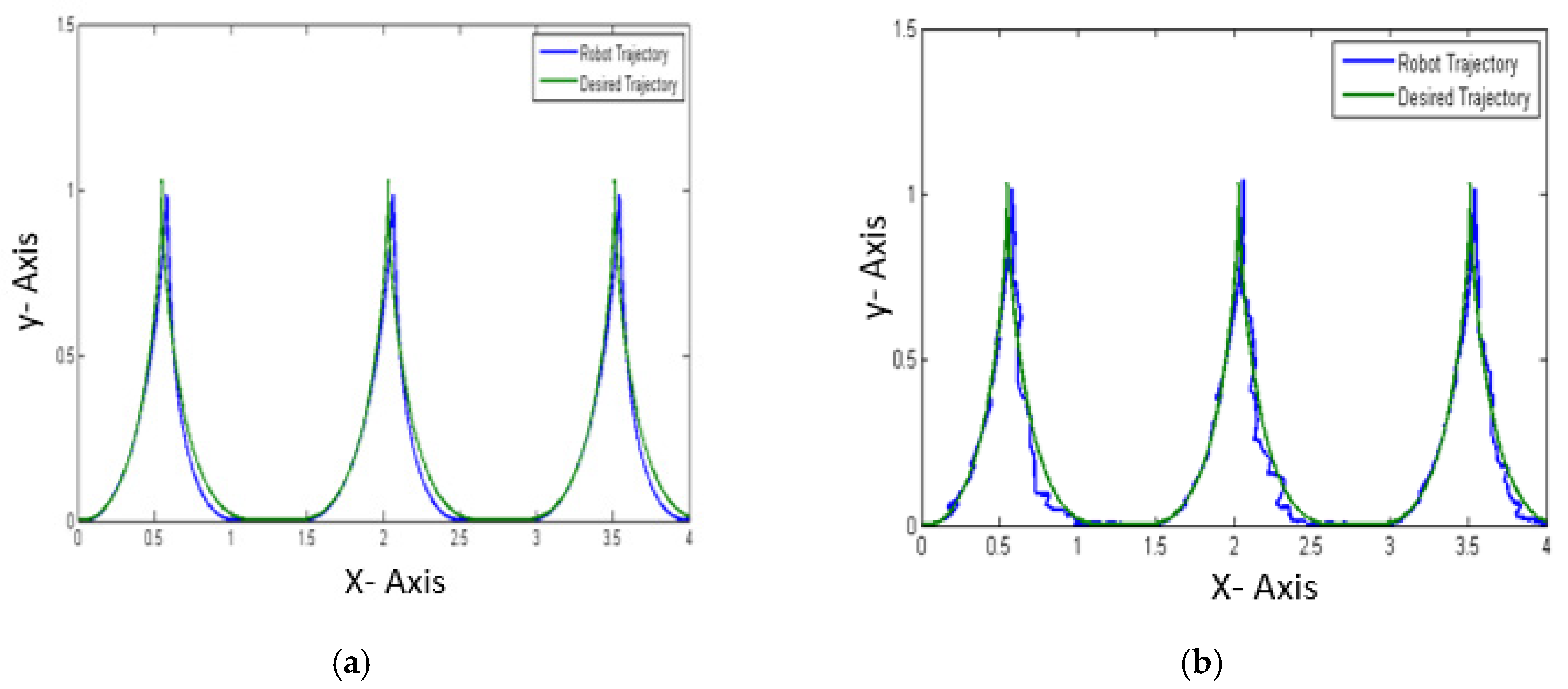
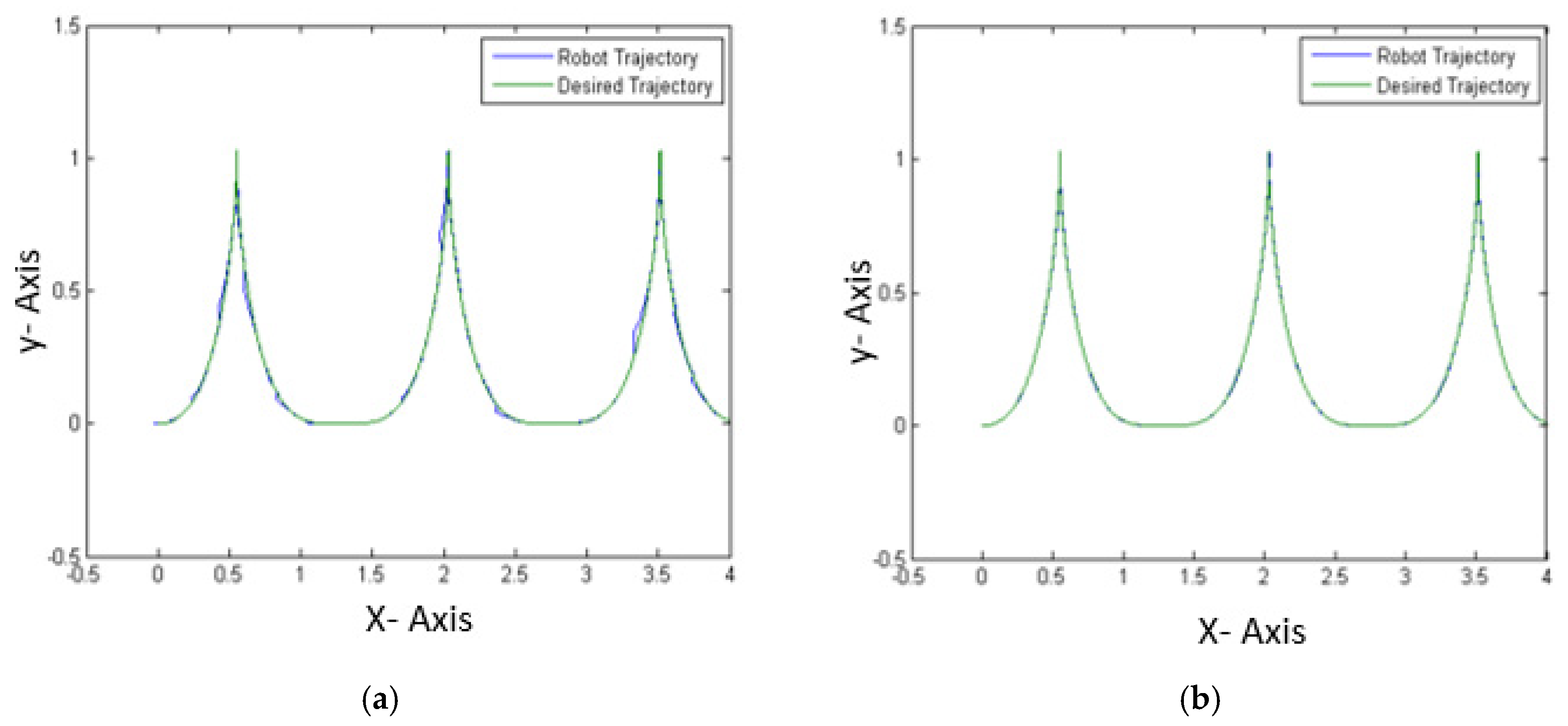
The main conclusions in this paper consist of highlighting the minimization of errors when the original algorithms are modified using the techniques of fuzzy logic. In both study cases in this paper, the proposed method demonstrates a stabilization and improvement with respect to the original algorithms. In this case, the proposed modification statistically shows in the mathematical functions a minimization of the error and, for the second problem of the mobile robot controller, stabilization in the trajectory even when noise is added in the model.

A comparison was presented between the two proposed methods in the case studies. In the first case of benchmark mathematical functions, OFHS achieves better results than OFDE. In the second case of control, both methods achieve good results by optimizing the robot controller with and without noise; in both cases, it is possible to minimize the error by applying noise to the controller. By comparing the results obtained with other existing methods in the literature, the effectiveness of the proposed methodology can be validated. The results obtained show the efficiency of the fuzzy logic system to find the optimal design in the membership functions (MFs) that allows the user to identify the values of the HMR and PArate parameters for the HS algorithm and the values of the F and CR parameters for the DE algorithm, and these values allow the user to obtain the modified algorithms that demonstrate a better performance in error minimization for the two study cases.

As to future work, we envision the implementation of this proposed method using interval type-2 fuzzy logic systems, as well as the experimentation with other non-linear models and being able to visualize the efficiency that this proposed method can demonstrate on the fuzzy control field.

References

1. Kim, J.H.; Geem, Z.W.; Jung, D.; Yoo, D.G.; Yadav, A. Advances in Harmony Search, Soft Computing and Applications; Springer International Publishing: Berlin, Germany, 2020. [Google Scholar]
2. Ceylan, O.; Sezgin, M.E.; Göl, M.; Verga, M.; Lazzari, R.; Kwaye, M.P.; Sandroni, C. Harmony Search Algorithm Based Management of Distributed Energy Resources and Storage Systems in Microgrids. Appl. Sci. 2020, 10, 3252. [Google Scholar] [CrossRef]
3. Daliri, S. Using Harmony Search Algorithm in Neural Networks to Improve Fraud Detection in Banking System. Comput. Intell. Neurosci. 2020. [Google Scholar] [CrossRef] [PubMed]
4. Gao, K.Z.; Suganthan, P.N.; Pan, Q.K.; Chua, T.J.; Cai, T.X.; Chong, C.S. Discrete harmony search algorithm for flexible job shop scheduling problem with multiple objectives. J. Intell. Manuf. 2016, 27, 363–374. [Google Scholar] [CrossRef]
5. Kayabekir, A.E.; Bekdaş, G.; Nigdeli, S.M.; Geem, Z.W. Optimum Design of PID Controlled Active Tuned Mass Damper via Modified Harmony Search. Appl. Sci. 2020, 10, 2976. [Google Scholar] [CrossRef]
6. Liu, L.; Huo, J.; Xue, F.; Dai, Y. Harmony Search Method with Global Sharing Factor Based on Natural Number Coding for Vehicle Routing Problem. Information 2020, 11, 86. [Google Scholar] [CrossRef] [Green Version]
7. Ouyang, H.B.; Gao, L.Q.; Li, S.; Kong, X.Y.; Wang, Q.; Zou, D.X. Improved harmony search algorithm: LHS. Appl. Soft Comput. 2017, 53, 133–167. [Google Scholar] [CrossRef]
8. Peraza, C.; Valdez, F.; Castillo, O. Harmony Search with Dynamic Adaptation of Parameters for the Optimization of a Benchmark Controller. In Intuitionistic and Type-2 Fuzzy Logic Enhancements in Neural and Optimization Algorithms: Theory and Applications; Springer: Cham, Switzerland, 2020; pp. 157–168. [Google Scholar]
9. Saha, S.; Ghosh, M.; Ghosh, S.; Sen, S.; Singh, P.K.; Geem, Z.W.; Sarkar, R. Feature Selection for Facial Emotion Recognition Using Cosine Similarity-Based Harmony Search Algorithm. Appl. Sci. 2020, 10, 2816. [Google Scholar] [CrossRef] [Green Version]
10. Talaei, K.; Rahati, A.; Idoumghar, L. A novel harmony search algorithm and its application to data clustering. Appl. Soft Comput. 2020, 92, 106273. [Google Scholar] [CrossRef]
11. Valdez, F.; Peraza, C.; Castillo, O. Study Cases to Test Fuzzy Harmony Search. In General Type-2 Fuzzy Logic in Dynamic Parameter Adaptation for the Harmony Search Algorithm; Springer: Cham, Switzerland, 2020; pp. 13–67. [Google Scholar]
12. Zhu, Q.; Tang, X.; Li, Y.; Yeboah, M.O. An improved differential-based harmony search algorithm with linear dynamic domain. Knowl. Based Syst. 2020, 187, 104809. [Google Scholar] [CrossRef]
13. Cui, L.; Li, G.; Lin, Q.; Chen, J.; Lu, N. Adaptive differential evolution algorithm with novel mutation strategies in multiple sub-populations. Comput. Oper. Res. 2016, 67, 155–173. [Google Scholar] [CrossRef]
14. Mohamed, A.W. A novel differential evolution algorithm for solving constrained engineering optimization problems. J. Intell. Manuf. 2018, 29, 659–692. [Google Scholar] [CrossRef]
15. Pholdee, N.; Bureerat, S.; Yıldız, A.R. Hybrid real-code population-based incremental learning and differential evolution for many-objective optimisation of an automotive floor-frame. Int. J. Veh. Des. 2017, 73, 20–53. [Google Scholar] [CrossRef]
16. Zhang, F.; Deb, C.; Lee, S.E.; Yang, J.; Shah, K.W. Time series forecasting for building energy consumption using weighted Support Vector Regression with differential evolution optimization technique. Energy Build. 2016, 126, 94–103. [Google Scholar] [CrossRef]
17. Yi, W.; Zhou, Y.; Gao, L.; Li, X.; Mou, J. An improved adaptive differential evolution algorithm for continuous optimization. Expert Syst. Appl. 2016, 44, 1–12. [Google Scholar] [CrossRef]
18. Zhou, Y.Z.; Yi, W.C.; Gao, L.; Li, X.Y. Adaptive differential evolution with sorting crossover rate for continuous optimization problems. IEEE Trans. Cybern. 2017, 47, 2742–2753. [Google Scholar] [CrossRef]
19. Ajeil, F.H.; Ibraheem, I.K.; Sahib, M.A.; Humaidi, A.J. Multi-objective path planning of an autonomous mobile robot using hybrid PSO-MFB optimization algorithm. Appl. Soft Comput. 2020, 89, 106076. [Google Scholar] [CrossRef] [Green Version]
20. Hoang Tran, T.; Duong Phung, M.; Viet Dang, A.; Tran, Q.V. Using multiple sensors for autonomous mobile robot navigation. arXiv 2020, arXiv:2005.06179. [Google Scholar]
21. Panda, M.R.; Panda, S.; Priyadarshini, R.; Das, P. Mobile Robot Path-Planning Using Oppositional-Based Improved Firefly Algorithm Under Cluttered Environment. In Advances in Intelligent Computing and Communication; Springer: Singapore, 2020; pp. 141–151. [Google Scholar]
22. Amador-Angulo, L.; Mendoza, O.; Castro, J.R.; Rodríguez-Díaz, A.; Melin, P.; Castillo, O. Fuzzy sets in dynamic adaptation of parameters of a bee colony optimization for controlling the trajectory of an autonomous mobile robot. Sensors 2016, 16, 1458. [Google Scholar] [CrossRef] [Green Version]
23. Nayyar, A.; Nguyen, N.G.; Kumari, R.; Kumar, S. Robot path planning using modified artificial bee colony algorithm. In Frontiers in Intelligent Computing: Theory and Applications; Springer: Singapore, 2020; pp. 25–36. [Google Scholar]
24. Cuevas, F.; Castillo, O. Design and implementation of a fuzzy path optimization system for omnidirectional autonomous mobile robot control in real-time. In Fuzzy Logic Augmentation of Neural and Optimization Algorithms: Theoretical Aspects and Real Applications; Springer: Cham, Switzerland, 2018; pp. 241–252. [Google Scholar]
25. Jain, S.; Sharma, V.K.; Kumar, S. Robot Path Planning Using Differential Evolution. In Advances in Computing and Intelligent Systems; Springer: Singapore, 2020; pp. 531–537. [Google Scholar]
26. Dzitac, I.; Filip, F.G.; Manolescu, M.J. Fuzzy logic is not fuzzy: World-renowned computer scientist Lotfi A. Zadeh. Int. J. Comput. Commun. Control. 2017, 12, 748–789. [Google Scholar] [CrossRef] [Green Version]
27. Lin, T.Y. Zadeh Sets-A” Perfect” Theory for Fuzzy Sets and Fuzzy Control: A First Outline. In Proceedings of the 2018 IEEE International Conference on Systems, Man, and Cybernetics (SMC), Miyazaki, Japan, 7–10 October 2018; pp. 3427–3433. [Google Scholar]
28. Vaidyanathan, S.; Azar, A.T. Takagi-Sugeno fuzzy logic controller for Liu-Chen four-scroll chaotic system. Int. J. Intell. Eng. Inform. 2016, 4, 135–150. [Google Scholar] [CrossRef]
29. Qais, M.H.; Hasanien, H.M.; Alghuwainem, S. Whale optimization algorithm-based Sugeno fuzzy logic controller for fault ride-through improvement of grid-connected variable speed wind generators. Eng. Appl. Artif. Intell. 2020, 87, 103328. [Google Scholar] [CrossRef]
30. Maalej, I.; Rekik, C.; Abid, D.B.H. Fault tolerant trajectory tracking control design for interval-type-2 Takagi-Sugeno fuzzy logic system. Int. J. Model. Identif. Control 2017, 27, 230–242. [Google Scholar] [CrossRef]
31. Kumar, A.; Saini, B. A Sugeno-Mamdani Fuzzy System Based Soft Computing Approach Towards Sensor Node Localization with Optimization. In International Conference on Next Generation Computing Technologies; Springer: Singapore, 2017; pp. 40–55. [Google Scholar]
32. Devi, M.S.; Soranamageswari, M. A hybrid technique of Mamdani and Sugeno based fuzzy interference system approach. In Proceedings of the 2016 International Conference on Data Mining and Advanced Computing (SAPIENCE), Ernakulam, India, 16–18 March 2016; pp. 340–342. [Google Scholar]
33. Civelek, Z. Optimization of fuzzy logic (Takagi-Sugeno) blade pitch angle controller in wind turbines by genetic algorithm. Eng. Sci. Technol. Int. J. 2020, 23, 1–9. [Google Scholar] [CrossRef]
34. Chouhan, A.S.; Parhi, D.R.; Chhotray, A. Control and Balancing of Two-Wheeled Mobile Robots Using Sugeno Fuzzy Logic in the Domain of AI Techniques. Emerging Trends in Engineering, Science and Manufacturing, (ETESM-2018); IGIT: Sarang, India, 2018. [Google Scholar]
35. Vrkalovic, S.; Teban, T.A.; Borlea, I.D. Stable Takagi-Sugeno fuzzy control designed by optimization. Int. J. Artif. Intell 2017, 15, 17–29. [Google Scholar]
36. Hussien, A.G.; Hassanien, A.E.; Houssein, E.H.; Amin, M.; Azar, A.T. New binary whale optimization algorithm for discrete optimization problems. Eng. Optim. 2020, 52, 945–959. [Google Scholar] [CrossRef]
37. Ochoa, P.; Castillo, O.; Soria, J. The Differential Evolution Algorithm with a Fuzzy Logic Approach for Dynamic Parameter Adjustment Using Benchmark Functions. In Hybrid Intelligent Systems in Control, Pattern Recognition and Medicine; Springer: Cham, Switzerland, 2020; pp. 169–179. [Google Scholar]
38. Peraza, C.; Valdez, F.; Castillo, O. Harmony Search with Dynamic Adaptation of Parameters for the Optimization of a Benchmark Set of Functions. In Hybrid Intelligent Systems in Control, Pattern Recognition and Medicine; Springer: Cham, Switzerland, 2020; pp. 97–108. [Google Scholar]
39. Rao, R. Rao algorithms: Three metaphor-less simple algorithms for solving optimization problems. Int. J. Ind. Eng. Comput. 2020, 11, 107–130. [Google Scholar] [CrossRef]
40. Sulaiman, M.H.; Mustaffa, Z.; Saari, M.M.; Daniyal, H. Barnacles Mating Optimizer: A new bio-inspired algorithm for solving engineering optimization problems. Eng. Appl. Artif. Intell. 2020, 87, 103330. [Google Scholar] [CrossRef]
41. Yue, X.; Zhang, H.; Yu, H. A Hybrid Grasshopper Optimization Algorithm with Invasive Weed for Global Optimization. IEEE Access 2020, 8, 5928–5960. [Google Scholar] [CrossRef]
42. Pérez, J.; Valdez, F.; Castillo, O. Bat algorithm comparison with genetic algorithm using benchmark functions. In Recent Advances on Hybrid Approaches for Designing Intelligent Systems; Springer: Cham, Switzerland, 2014; pp. 225–237. [Google Scholar]
43. Mulo, T.; Syam, P.; Choudhury, A.B. Application of Modified Harmony Search and Differential Evolution Optimization Techniques in Economic Load Dispatch. In Advances in Control, Signal Processing and Energy Systems; Springer: Singapore, 2020; pp. 199–213. [Google Scholar]
44. Storn, R.; Price, K. Differential evolution–a simple and efficient heuristic for global optimization over continuous spaces. J. Glob. Optim. 1997, 11, 341–359. [Google Scholar] [CrossRef]
45. Geem, Z.W.; Kim, J.H.; Loganathan, G.V. A new heuristic optimization algorithm: Harmony search. Simulation 2001, 76, 60–68. [Google Scholar] [CrossRef]
46. Castillo, O.; Valdez, F.; Soria, J.; Amador-Angulo, L.; Ochoa, P.; Peraza, C. Comparative study in fuzzy controller optimization using bee colony, differential evolution, and harmony search algorithms. Algorithms 2019, 12, 9. [Google Scholar] [CrossRef] [Green Version]
47. Martínez, R.; Castillo, O.; Aguilar, L.T. Intelligent control for a perturbed autonomous wheeled mobile robot using type-2 fuzzy logic and genetic algorithms. J. Autom. Mob. Robot. Intell. Syst. 2008, 2, 12–22. [Google Scholar]
48. Martínez, R.; Castillo, O.; Aguilar, L.T. Optimization of interval type-2 fuzzy logic controllers for a perturbed autonomous wheeled mobile robot using genetic algorithms. Inf. Sci. 2009, 179, 2158–2174. [Google Scholar] [CrossRef]
49. Castillo, O.; Neyoy, H.; Soria, J.; Melin, P.; Valdez, F. A new approach for dynamic fuzzy logic parameter tuning in ant colony optimization and its application in fuzzy control of a mobile robot. Appl. Soft Comput. 2015, 28, 150–159. [Google Scholar] [CrossRef]
50. Castillo, O.; Martínez-Marroquín, R.; Melin, P.; Valdez, F.; Soria, J. Comparative study of bio-inspired algorithms applied to the optimization of type-1 and type-2 fuzzy controllers for an autonomous mobile robot. Inf. Sci. 2012, 192, 19–38. [Google Scholar] [CrossRef]
Figure 1. Proposed method.
Applsci 10 06146 g001
Figure 2. Points of triangular membership function.
Applsci 10 06146 g002
Figure 3. Parameters of the membership functions for Input 1 and Input 2.
Applsci 10 06146 g003
Figure 4. Parameters of the membership functions of the Output 1 and Output 2.
Applsci 10 06146 g004
Figure 5. Vector for the optimization optimized fuzzy differential evolution (OFDE) and optimal fuzzy harmony search (OFHS).
Applsci 10 06146 g005
Figure 6. Diagram of the robot mobile controller.
Applsci 10 06146 g006
Figure 7. Points of trapezoidal membership function.
Applsci 10 06146 g007
Figure 8. Points membership functions of Input 1 and Input 2.
Applsci 10 06146 g008
Figure 9. Surface of the mobile robot controller.
Applsci 10 06146 g009
Figure 10. Vector for the fuzzy logic controller.
Applsci 10 06146 g010
Figure 11. Best simulation OFDE (a) without noise and (b) with noise.
Applsci 10 06146 g011
Figure 12. Best simulation OFHS (a) without noise and (b) with noise.
Applsci 10 06146 g012