A Novel Pipeline Leak Recognition Method of Mine Air Compressor Based on Infrared Thermal Image Using IFA and SVM

Abstract

In order to accurately identify the pipeline leak fault of a mine air compressor, a novel intelligent diagnosis method is presented based on the integration of an adaptive wavelet threshold denoising (WTD) algorithm, improved firefly algorithm (IFA), Otsu-Grabcut image segmentation algorithm, histogram of oriented gradient (HOG), gray-level co-occurrence matrix (GLCM) and support vector machine (SVM). In the proposed method, the adaptive step strategy and local optimal firefly self-search strategy for the basic firefly algorithm (FA) are used to improve the optimization effect. The infrared thermal image is denoised by using wavelet threshold algorithm which is optimized by IFA (WTD-IFA). The Otsu-Grabcut algorithm is used to segment the image and extract the target. The HOG and GLCM are calculated to reveal the intrinsic characteristics of the infrared thermal image to extract feature vectors. Then the IFA is utilized to optimize the parameters of SVM so as to construct an optimal classifier for fault diagnosis. Finally, the proposed fault diagnosis method is fully evaluated by experimentation and the results verify its feasibility and superiority.

1. Introduction

Mine air compressors are important equipment for guaranteeing safety. Compressed air is transported underground through seamless steel pipes. On one hand, compressed air provides power for wind hammers, air pumps and other mine pneumatic equipment [1]. On the other hand, it can ensure that there is enough oxygen underground to protect the lives of coal miners [2]. Due to the high-pressure characteristics of compressed air, compressed air often leaks from the gas delivery pipeline during operation. According to statistics, there is a serious loss of compressed air during production and utilization, which accounts for about 25% to 30% of the total demand for compressed air [3]. In some specific systems, the loss rate even reaches 30% to 60% [4]. Leakage is the most obvious and important reason for the loss of compressed air, which can reach 20% to 40% of the total gas usage [5]. If the compressed air leaks in a very short time, it will not only cause huge economic losses, but also cause equipment damage and endanger personal safety. At present, the detection of such faults mainly depends on worker’s hearing and observation to determine whether the pipeline is leaking. Obviously, the detection efficiency is very low and the leak fault cannot be found in time. In addition, the air temperature and noise in the compressor room is very hostile. It is extremely critical to discover and eliminate the compressed air leak faults early when the faults occur. Therefore, the research of compressed air leak fault diagnosis technology for mine pipes is of great significance and practical value.

In recent decades, many experts and researchers have proposed two general leak fault monitoring methods. The first is to detect the substance that escapes from the pipe. A sensor is used to detect the leaking substance, which should be contacted with this substance and be close to the leak. This requires a dense concentration of sensors. Thus, for a long pipeline, the method will yield a large number of remote units and high costs. The second way is to detect certain leak-related properties such as pressure drops, acoustic emissions, volume balance changes and temperature changes. Temperature monitoring and volume balance comparison (comparing the amount of material injected into the pipe to the amount received from the pipe) techniques are useful for the detection of large or catastrophic leaks, and have been widely used in many fields. However, these systems are not sensitive to small leaks.

At present, the detection methods for pipeline gas leakage are mainly based on acoustic, ultrasonic and infrared technologies. Madding et al. [6] used an infrared camera to detect the leakage of SF6 gas, improving the detection efficiency. Slobodan Dudić et al. [7] used ultrasound and infrared thermography technology to detect the leakage of compressed air, and found that thermography can offer good results for the leakage quantification from orifices greater than 1.0 mm and ultrasound should be used for leakage detection for all dimensions of orifices. Lingya Meng et al. [8] conducted an experimental study on the detection and location of natural gas pipeline leaks based on acoustic methods. The wavelet transform was used to reduce the noise of the acoustic signal collected by the sensor, which improved the recognition sensitivity of the system. Marcia Golmohamad [9] used ultrasound to study the pipeline leak detection technology. However, this method cannot perform real-time inspection on the pipeline at work, and is only suitable for inspection before the pipeline is used. Yonghong Wang [10] used the basic principle of ultrasonic detection of pressure vessel leakage, wavelet analysis and BP neural network to identify the gas leakage signal. Jin Hao et al. [11] proposed a method for detecting and locating natural gas pipeline leaks based on the sonic method. It can be seen that the traditional gas leak detection methods cannot effectively detect the gas leak on time and cannot meet the accuracy demand of fault diagnosis.

The infrared images of compressed air leak pipes contain information about temperature changes caused by compressed air leaks. However, the infrared image cannot directly display the characteristics of leaked compressed air due to presence of the atmospheric window [12]. Therefore, how to use appropriate mean to introduce the intelligent algorithms into the compressed air leak detection is a problem that needs to be studied deeply. In order to ensure the leak recognition effect, the infrared image technology is integrated with some related methods, such as wavelet threshold denoising (WTD), firefly algorithm (FA), Otsu’s method, Grabcut, histogram of oriented gradient (HOG), gray-level co-occurrence matrix (GLCM) and support vector machine (SVM). These methods have their own advantages and disadvantages in actual applications. For example, wavelet threshold denoising can decompose the signal into high and low frequencies, and remove part of the high frequencies to denoise the signal, but it is not suitable to decompose the high frequency, and hard to find the optimal threshold. The FA is simple and easy to implement and has fast solving speed, but it is easy to fall into local extreme point. The Otsu’s method is easy to separate the pixels of one picture into two classes, foreground and background, but it returns a binary image. The Grabcut is an easy image segmentation method based on graph cuts, but it has to point out the misclasses regions by user. The HOG can describe the local shape information of the image, but it is quite sensitive to noise. The GLCM can describe texture features, but small changes in the image can cause large changes in the energy distribution. The SVM can solve the small-sample, nonlinear and high-dimensional problems, but when it is used to solve nonlinear problems, the selection of kernel function directly affects the final classification result. Therefore, in order to effectively recognize the pipeline leak, the WTD, IFA, Otsu-Grabcut, HOG-GLCM and SVM are fully integrated to propose a novel intelligent diagnosis method for compressed air leaks. Furthermore, the IFA is used to optimize the parameters of the WTD (WTD-IFA) for better denoising efforts. Otsu-Grabcut is used to segment the picture to remove the irrelevant information. The HOG-GLCM is used to effectively extract the leak fault features, and the IFA is used to optimize the parameters of SVM to establish an optimal SVM classifier with high classification accuracy.

2. Materials and Methods

2.1. Firefly Algorithm and Its Improvements

2.1.1. Classic Firefly Algorithm

Firefly Algorithm (FA) is a swarm intelligence optimization algorithm proposed by Xin-She Yang in 2008 to simulate the group behavior of fireflies [13]. The classic firefly algorithm uses the mutual attraction of fireflies to affect the movement of firefly groups, and has a stronger local attraction feature than the global optimal attraction. The firefly algorithm has few parameters, simple principle and easy operation. When the algorithm is running, the fireflies will automatically be divided into multiple small groups, which makes FA very suitable for nonlinear optimization problems, such as multi-peak, feature extraction, clustering, etc. Therefore, FA is increasingly used to solve important optimization problems in engineering and scientific fields, such as network, image processing, robot trajectory planning and text selection [14,15,16]. However, FA also has some defects such as low convergence accuracy, slow convergence speed at the end of the iteration, and is difficult to be away from local optimality [17,18,19,20,21]. In order to improve the ability of FA, many research scholars have transformed FA, and there are two main ideas for improvement. One is to optimize the parameters of FA, and the other is to combine the excellent ideas of other group optimization algorithms with FA to obtain better search capabilities. Xin-She Yang [22] proposed the Levy-flight Firefly Algorithm (LFA), which absorbed the distribution characteristics of the long tail in the Levy flight algorithm, and improved the update step strategy of the firefly algorithm. Afnizanfaizal [23] combines the idea of differential evolution with FA. He gathered the poor fireflies together to form new populations, and updated the coordinates of the fireflies through differential evolution, thereby improving the ability of the algorithm to remove local optimality, called the hybrid evolution firefly algorithm (HEFA).

The steps of the classic firefly algorithm are as follows:

• FA parameters initialization. First, we set the size of the solution space to D, then set an appropriate number of fireflies N according to D. The maximum update number tmax is set appropriately, and the appropriate absorption coefficient $\Upsilon$ is set according to different media, usually 1; the initial step size s is usually set to 0.5. The initial attraction β₀ represents the attraction at the light source (distance r = 0), usually set to 1, and the coordinate of the i-th firefly is expressed as X_i= (x_i1, x_i2, …, x_iD).
• Firefly’s attractiveness calculation. According to the coordinates of each firefly and the corresponding fitness evaluation function, the fitness of the firefly is calculated as the brightness of the fireflies. The aim of the firefly algorithm is to find the optimal solution in the objective function, and the brightness of the firefly’s position is the firefly’s solution in the objective function. When the function is known, the brightness of the firefly can be obtained by introducing the position coordinates of the firefly, which can be used to judge the position of the firefly. Then, based on the brightness, the absorption coefficient and the distance between fireflies the attraction β between fireflies is calculated, as shown below:

  $$\{\begin{array}{l}\beta (r_{ij})={\beta }_0\times e^{-\Upsilon r_{ij}^2}\\ r_{ij}=\Vert x_i-x_j\Vert \end{array},$$

  (1)

  where r_ij is the distance between two fireflies.

Fireflies’ location update. According to the calculated attraction, each firefly flies to a more attractive firefly. The update step calculation formula for the t-th generation fireflies is as follows:

$$s(t)=s^t\cdot {\epsilon }^t,$$

(2)

where s^t stands for the t-th step, ε^t represents the random coefficient of the t-th generation obeying uniform distribution.

The firefly position update equation is written as follows:

$$x_i^{t+1}=x_i^t+\beta (r_{ij})(x_j^t-x_i^t)+s(t),$$

(3)

3.

Location update judgment. The brightness of the firefly at the new position is calculated. If the brightness of the firefly is brighter, the firefly’s position will be updated, otherwise, it will not be updated.

4.

Algorithm iteration. According to steps (2)–(4), fireflies will be updated through multiple flights until the maximum number of iterations is reached, and one or more firefly clusters will eventually be formed. The coordinates of the brightest firefly represent the optimal solution that the algorithm finds in this space.

After clarifying the problem of the standard firefly algorithm, this paper proposes some improved measures for the shortcomings of FA.

2.1.2. Improved Firefly Algorithm

In order to solve the problem of early convergence and local extremum, this paper proposes an improved firefly algorithm (IFA). The main idea of the improved strategy is as follows:

• Firefly’s update efficiency is improved. When the step size is updated, a fixed distribution step size is used in the classical algorithm. The updated strategy is consistent at different stages of the algorithm. Therefore, it was decided to introduce a step size range to limit the uniform distribution, so that the step size range will decrease as the number of updates increase. In the early stage, the firefly update step size is larger and rapid iterations are performed. As the iterations increase, the firefly update step size becomes smaller, which enhances the local search capability, and finally achieves the purpose of optimizing the algorithm. The updated step method of IFA is as follows:

  $$s(t)=s^t\cdot {\epsilon }^t\cdot \left(\cos \left(\frac{\pi t}{t_{max}}\right)+1\right),$$

  (4)
• The self-search ability of the local optimal firefly is improved. Because all firefly individuals only fly to fireflies which are brighter than themselves, the brightest individual in the group does not move, but there is no guarantee that the individual is in the optimal position. In response to such problems, the firefly in the optimal position is randomly searched in an adaptive circle centered on itself and the radius gradually decreases as the number of iterations increases. If the brightness of the firefly is brighter in the new location, the coordinates of the firefly will be updated, otherwise it is not updated, Therefore, the self-search ability of fireflies to the surrounding environment has been improved, and fireflies can jump out from the local optimal position. The optimal firefly self-search update formula is as follows:

  $$x_i^{t+1}=x_i^t+{\Upsilon }^t\cdot \cos \left(\frac{\pi t}{2t_{max}}\right)\cdot {\epsilon }^t,$$

  (5)

  where the ${\Upsilon }^t\cdot \cos \left(\frac{\pi t}{2t_{max}}\right)$ represents the self-searching range of the optimal firefly at the t-th iteration.

The optimized firefly algorithm implementation process is shown Figure 1.

2.1.3. Simulation Analysis

In order to verify the superiority of IFA, this paper selects 8 standard test functions to test standard FA, LFA and IFA, respectively, as shown in

Table 1. Standard test functions.

	Function Name	Dimension	Independent Variable Value Range	Function Formula	Theoretical Value
f1	Ackley	2	[−32.768, 32.768]	$\begin{array}{l}f\left(x\right)=-20\exp \left(-0.2\sqrt{\frac{1}{d}{\displaystyle \sum _{i=1}^d{x}_i{}^2}}\right)\\ -\exp \left(\frac{1}{d}{\displaystyle \sum _{i=1}^d\cos \left(2\pi x_i\right)}\right)+\exp \left(1\right)\end{array}$	fmin = 0
f2	Cross in Tray	2	[−10, 10]	$f\left(x\right)=-0.0001{\left(t+1\right)}^{0.1}$ $t=\left|\sin \left(x_1\right)\sin \left(x_2\right)\exp \left(\left|100-\frac{\sqrt{x_1^2+x_2^2}}{\pi }\right|\right)\right|$	fmin = −2.06261
f3	Drop Wave	2	[−5.12, 5.12]	$f\left(x\right)=-\frac{1+\cos \left(12\sqrt{x_1^2+x_2^2}\right)}{0.5\left(x_1^2+x_2^2\right)+2}$	fmin = −1
f4	Griewank	2	[−600, 600]	$f\left(x\right)={\displaystyle \sum _{i=1}^d\frac{x_i^2}{4000}-{\displaystyle \prod _{i=1}^d\cos \left(\frac{x_i}{\sqrt{i}}\right)+1}}$	fmin = 0
f5	Levy 13	2	[−10, 10]	$\begin{array}{l}f\left(x\right)={\sin }^2\left(3\pi x_1\right)+{\left(x_1-1\right)}^2\left[1+{\sin }^2\left(3\pi x_2\right)\right]\\ +{\left(x_2-1\right)}^2\left[1+{\sin }^2\left(2\pi x_2\right)\right]\end{array}$	fmin = 0
f6	Rastrigin	2	[−5.12, 5.12]	$f\left(x\right)=10d+{\displaystyle \sum _{i=1}^d\left[x_i^2-10\cos \left(2\pi x_i\right)\right]}$	fmin = 0
f7	Booth	2	[−10, 10]	$f\left(x\right)={\left(x_1+2x_2-7\right)}^2+{\left(2x_1+x_2-5\right)}^2$	fmin = 0
f8	Three Hump Camel	2	[−5, 5]	$f\left(x\right)=2x_1^2-1.05x_1^4+\frac{x_1^6}{6}+x_1{x}_2+x_2^2$	fmin = 0

.

The unified maximum iteration number is set to 200, absorption coefficient γ = 1, initial step size s = 0.5, initial attraction β₀= 1, and the number of random fireflies is 20. The test experiments are conducted 30 times for each algorithm, and the best value, the best value variance and the average running times are recorded. The iteration curves are shown in Figure 2, and the simulation results are shown in

Table 2. Comparison of optimal values and variance. FA: firefly algorithm.

	Parameter	Optimal Value			Optimal Value Variance
Function		FA	LFA	IFA	FA	LFA	IFA
f1		1.02 × 10−4	0.00452104	5.92 × 10−4	0.97116936	0.13558556	1.83 × 10−5
f2		−2.06261	−2.06261	−2.06261	6.21 × 10−6	2.18 × 10−7	3.43 × 10−13
f3		−1.00	−0.999951	−0.999984	0.0280539	8.28 × 10−4	9.32 × 10−4
f4		7.79× 10−8	2.45× 10−5	7.11 × 10−8	1.37 × 10−5	1.33 × 10−5	1.36 × 10−5
f5		1.83 × 10−7	3.24 × 10−5	2.80 × 10−8	0.858863	9.74 × 10−4	2.31 × 10−11
f6		7.60 × 10−5	0.001572	1.94 × 10−7	1.33	0.15732	0.0329
f7		2.80 × 10−8	3.57 × 10−5	1.73 × 10−7	0.010723	0.006544	2.11 × 10−11
f8		6.35 × 10−8	8.27 × 10−6	3.36 × 10−7	0.005363	3.27 × 10−6	1.42 × 10−8

and

Table 3. Comparison of average running time.

	Parameter	The Average Operation Time (s)
Function		FA	LFA	IFA
f1		0.2729	0.2769	0.2608
f2		0.2659	0.2631	0.240933
f3		0.24796	0.2591667	0.2313333
f4		0.258367	0.252167	0.247967
f5		0.255033	0.2588	0.230233
f6		0.261667	0.269767	0.233567
f7		0.2536	0.259767	0.2281
f8		0.270467	0.258633	0.2308

.

As shown in Figure 2, the IFA algorithm proposed in this paper has achieved good results in the search for the global optimal process in different test functions, and the convergence speed is the fastest. IFA has a stronger ability to jump out of local optimality than the other two algorithms. As shown in Table 3, the accuracy of the optimal output value of IFA is higher, which basically belongs to the same level as the FA algorithm, and the accuracy of LFA optimal value search is lower. From the perspective of variance values, the variance values of the IFA algorithm are much smaller than those of the FA algorithm and LFA, indicating that the IFA algorithm is very stable and has a very high robustness. As shown in

Table 4. The configuration and parameters of processing platform.

Type	Parameter
System	Windows10 (64bit)
Central processing unit (CPU)	AMD Ryzen 5 3500 u 2.10 GHz
Random access memory (RAM)	16 GB
Read only memory (ROM)	SSD (512 GB)
Matlab version	2019b

, the operation time of the IFA algorithm is the shortest. In summary, the IFA algorithm has achieved the best results in terms of convergence speed, calculation accuracy, robustness, and calculation speed, and is particularly prominent in terms of robustness and calculation speed.

2.2. Principle of Wavelet Threshold Denoising

The current commonly used image denoising methods include median filtering, bilateral filtering [24], Block-Matching 3-Dimension (BM3D) [25], wavelet threshold denoising [26], etc. In the method of wavelet threshold image denoising, the key is to calculate the appropriate wavelet threshold. If the selected threshold is too large, the removed information will contain noise and valid information, which will reduce the imaging quality. Conversely if the threshold is too small, the noise in the image cannot be removed clearly. The noise in the image mainly comes from the electromagnetic wave interference from the environment and the photoelectric, mechanical, material, circuit and other noise of the imaging system. Assuming that the noise of the image is independent of the original image, the noise can usually be divided into additive noise and multiplicative noise:

$$Y_{ij}=X_{ij}\cdot \delta +N_p,$$

(6)

where X_ij is noise-free image; Y_ij is noisy images; δ is multiplicative noise and N_p is additive noise.

For a noisy image, the additive and multiplicative noises in the image need to be filtered to obtain a noise-free image. Wavelet transform can decompose the image on multiple scales, which is more conducive to separating noise. Therefore, wavelet transform has great advantages in removing image noise.

2.2.1. Wavelet Threshold Denoising

The definitions of continuous wavelet transform and inverse transform are as follows:

$$W_T\left(a,b\right)=\frac{1}{\sqrt{a}}{\displaystyle {\int }_{-\infty }^{+\infty }x\left(t\right)\cdot \psi \left(\frac{t-b}{a}\right)dt},$$

(7)

$$x\left(t\right)=\frac{1}{C_{\phi }}{{\displaystyle {\int }_{-\infty }^{+\infty }{\displaystyle {\int }_{-\infty }^{+\infty }{W}_T\left(a,b\right){\psi }_{a,b}\left(t\right)}}}^2{a}^{-2}dadb,$$

(8)

where $C_{\phi }={\displaystyle \int \frac{{\left|\psi \left(w\right)\right|}^2}{\left|w\right|}}dw<+\infty$, x(t) stands for the image to be processed, ψ(t) represents the wavelet function, a is expansion coefficient, b is translation value.

In fact, the continuous wavelet transform theory is mainly used in theoretical research. In practical application, the scale parameter a and translation parameter b need to be discretized. Normally, $a=a_0^j$, $a=k{b}_0{a}_0^j$, and a₀ > 1, b₀ > 0, j and k are rounded. The definition of discrete wavelet is as follows:

$${\phi }_{j,k}=\frac{1}{\sqrt{a_0^j}}\phi \left(\frac{t-k{b}_0{a}_0^j}{a_0^j}\right)=a_0^{-j/2}\phi \left(a_0^{-j}t-k{b}_0\right)$$

(9)

The corresponding discrete wavelet transform is as follows:

$$W_T\left(j,k\right)=a_0^{-j/2}{\displaystyle {\int }_{-\infty }^{+\infty }T\left(t\right)}{\phi }_{j,k}\left(t\right)dt=a_0^{-j/2}{\displaystyle {\int }_{-\infty }^{+\infty }T\left(t\right)}\phi \left(a_0^{-j}t-k{b}_0\right)dt$$

(10)

In practical application, the commonly used discrete method is to discretize a and b, so a₀ = 2, b₀ = 1. The discrete wavelet is as follows:

$${\phi }_{j,k}\left(t\right)=2^{-j/2}\phi \left(2^{-j/2}t-k\right)$$

(11)

Since the image is a two-dimensional spatial signal, it is necessary to extend one-dimensional wavelet transform into two-dimensional wavelet transform.

The wavelet threshold image denoising process is as follows:

(1)

Wavelet transform. For noisy images, we select a suitable wavelet function, and use the wavelet function to perform multi-layer decomposition of noisy images through wavelet transform to obtain a set of wavelet coefficients.

(2)

Non-linear threshold. According to the characteristics of the noise in the noisy image, an appropriate noise threshold is selected through a threshold function, and the wavelet coefficients of the noise part in the high-frequency decomposition value are reset to zero. Commonly used threshold functions are hard threshold function, soft threshold function and semi-soft threshold function. The hard threshold function is given as follows:

$$\overline{W_{j,k}}=\{\begin{array}{ll}{W}_{j,k}& ,\left|W_{j,k}\ge \tau \right|\\ 0& ,\left|W_{j,k}<\tau \right|\end{array}.$$

(12)

The soft threshold function is as follows:

$$\overline{W_{j,k}}=\{\begin{array}{cc}\mathrm{sgn}\left(W_{j,k}\right)\left(\left|W_{j,k}\right|-\tau \right)& ,\left|W_{j,k}\ge \tau \right|\\ 0& ,\left|W_{j,k}<\tau \right|\end{array}.$$

(13)

The semi-soft threshold function is as follows:

$$\overline{W_{j,k}}=\{\begin{array}{cc}\mathrm{sgn}\left(W_{j,k}\right)\left|W_{j,k}\right|-\tau +\frac{2\tau }{1+e^{2W_{j,k}/\tau }}& ,\left|W_{j,k}\ge \tau \right|\\ 0& ,\left|W_{j,k}<\tau \right|\end{array}.$$

(14)

where $\overline{W_{j,k}}$ is wavelet shrinkage coefficient; $W_{j,k}$ is wavelet coefficient; sgn() stands for the symbolic function and τ is the wavelet threshold.

(3)

Inverse wavelet transform to reconstruct the image. The processed wavelet estimation coefficients are subjected to inverse wavelet transform to obtain a noise-removed image.

In this paper, an improved firefly algorithm is used to search the optimal wavelet threshold of the denoised image in the global range through iterative optimization to improve the denoising effect of the denoising algorithm. The wavelet coefficients processed by the hard threshold function will have a discontinuous function near the threshold, the wavelet coefficients processed by the soft threshold function are prone to deviation, resulting in blurred edges. Therefore, the semi-soft threshold function is used to process the wavelet threshold searched by the improved firefly algorithm.

2.2.2. WTD-IFA

Combining IFA and wavelet threshold denoising algorithm (WTD), an adaptable wavelet threshold infrared image denoising algorithm (WTD-IFA) is proposed. For swarm intelligence algorithms, it is necessary to establish a fitness function to evaluate the quality of the denoising effect. In this paper, the purpose of denoising the infrared image is to decompose the infrared image containing noise into a noise signal and a relatively pure image signal. It is generally believed that the smaller the correlation between the noise signal and the image signal, the better, so the reconstructed correlation coefficient between the image and the noise signal separated by denoising is used as a fitness function. The purpose of decomposing the image to remove noise is achieved by reducing the value of the fitness function. The fitness function is as follows:

$$f_{rn}=corr\left(R,N\right),$$

(15)

where the f_rn stands for the correlation coefficient between the reconstructed image and separated noise signal; R is the reconstructed image and N is the separated noise signal.

The filter realization process based on WTD-IFA is as follows:

(1)

Wavelet decomposition. Wavelet transform is used to decompose the infrared image with noise.

(2)

Threshold initialization. Initializing the IFA threshold and initializing the firefly position (wavelet threshold).

(3)

The wavelet coefficients contract. Equation (6) is used to calculate the wavelet contraction coefficient, and the image is reconstructed based on the wavelet contraction coefficient.

(4)

Firefly algorithm iteration. The fitness of the reconstructed image is calculated according to Equation (12). If the iteration number of the firefly algorithm is greater than 1, it is judged whether the fitness of the firefly is better than the fitness of the original position. If yes, the firefly position is updated, otherwise, the firefly position is kept unchanged. If the image fitness result meets the termination condition, execute step (6), otherwise execute step (5).

(5)

Firefly location update. Based on the firefly’s current fitness value and the IFA’s location update rules, the firefly’s new location is calculated. Then go to step (3).

(6)

Image reconstruction. The image is reconstructed using the global optimal wavelet threshold searched by WTD-IFA.

The flowchart of the WTD-IFA algorithm is shown in Figure 3.

In this paper, the wavelet basis function is sym4, and the noisy image is decomposed by 5-level 2D static discrete wavelet transform.

2.3. Image Segmentation and Feature Extraction

2.3.1. Otsu-Grabcut Algorithm

At present, the most widely used image segmentation algorithm is the threshold segmentation algorithm, which includes global threshold segmentation and local threshold segmentation. The Otsu method, also known as the maximum between-class variance method, was proposed by the Japanese scholar Otsu [27] in 1979. The original Otsu is an adaptive global threshold segmentation method. The algorithm calculates the best threshold in the image and improves the image. The distinction between the background and target pixels is maximized, so as to achieve the purpose of extracting the target in the image. However, for infrared images, the grayscale distribution of the image is more complicated, and the traditional Otsu method is not good at segmentation. Therefore, some scholars have proposed an improved Otsu algorithm based on a two-dimensional histogram. As the horizontal axis, the average gray value of the neighboring pixels is used as the vertical axis to form a two-dimensional histogram. When searching for the threshold, the spatial correlation information of the image is fully used. Therefore, the algorithm has a good segmentation effect for infrared images.

The Otsu algorithm based on the two-dimensional histogram uses the neighborhood deviation m(x, y) to represent the deviation between the gray value of the pixel and the average gray of the neighborhood. The calculation formula is shown as follow:

$$m\left(x,y\right)=\frac{\sqrt{\left|f\left(x,y\right)-v\left(x,y\right)\right|}}{v\left(x,y\right)},$$

(16)

where f(x, y) is the gray value of pixels, v(x, y) is the average gray level of all pixels in the neighborhood with (x, y) as the center pixel.

However, the segmented image is a binary image, and a lot of information in the original image is lost. Therefore, a new algorithm combining the two-dimensional Otsu algorithm and Grabcut extraction algorithm is proposed to process the infrared image.

2.3.2. Grabcut Algorithm

Grabcut is a graph-based segmentation method, which is an improvement to the Graphcut algorithm [28]. The Grabcut algorithm is based on the Red-Green-Blue (RGB) three-channel mixed Gaussian model. It only needs to confirm the foreground and background in the image to complete the segmentation between the foreground and background. The Otsu algorithm can calculate the edge of the infrared image and determine the foreground in the image, that is, the detection target. Using the coordinate range of the target in the binary map calculated by the Otsu algorithm as the foreground input in the Grabcut algorithm, the original image can be segmented. The Grabcut algorithm needs to manually circle the foreground target, and it can cover a small amount of background information within the range.

The Grabcut algorithm uses a Gaussian mixture model to build a data model for the background and foreground regions. Assuming that there are N pixels in the figure, the points selected in the frame are first regarded as the target pixel Pt belongs to the foreground Gaussian mixture model, and the points outside the frame are regarded as the background pixel P_b belongs to the background Gaussian mixture model, calculated for each pixel The Gaussian components corresponding to other pixels are stored in the vector k = (k₁, k₂, …, k_N), and each pixel corresponds to a unique Gaussian component. When the pixel belongs to the front scenic spot, let = 0; when the pixel belongs to the background spot, let = 1, the algorithm continues to iterate until the energy E reaches the minimum to obtain the current segmentation boundary.

2.3.3. Otsu-Grabcut Image Segmentation Algorithm

In order to get a better automatic image segmentation effect, the Otsu and Grabcut algorithm are combined to propose the Otsu-Grabcut image segmentation algorithm. First, we use the Otsu algorithm to identify the edge of the target in the infrared image and record the coordinates of the target edge pixel. Then the coordinates of the image target are input into the Grabcut algorithm to complete the segmentation of the infrared image. The segmentation result of Otsu-Grabcut algorithm is shown in Figure 4. The key part of the infrared image is segmented, and the pipes and valves in the image are extracted, and the irrelevant background is removed completely.

2.4. Image Feature Extraction

2.4.1. Histogram of Oriented Gradient (HOG)

In image recognition, the histogram of oriented gradient (HOG) can be used to describe the characteristics of the image. This method calculates the statistics of the pixel distribution in the target image, and uses the gradient distribution characteristics and directional density distribution of the pixel values in the figure to describe the texture and boundary in the image. The calculation method of HOG features is as follows:

For color images, it is necessary to first perform gray processing and gamma correction on the gray images, which is helpful to reduce the influence of uneven distribution of light intensity and noise on texture features in the image.

(1)

Calculation of pixel distribution gradient. Common forms of simple convolution are [−1,0,1] and [−1,0,1]^T. Convolution calculation is performed on the preprocessed image to generate two orthogonal gradient components, and the gradient direction of each pixel can be calculated according to the component. The calculation formula is shown as follow:

$$\{\begin{array}{c}G\left(x,y\right)=\sqrt{G_x{\left(x,y\right)}^2+G_y{\left(x,y\right)}^2}\\ M\left(x,y\right)={\tan }^{-1}\left(G_y\left(x,y\right)/G_x\left(x,y\right)\right)\\ G_x\left(x,y\right)=H\left(x+1,y\right)-H\left(x-1,y\right)\\ G_y\left(x,y\right)=H\left(x,y+1\right)-H\left(x,y-1\right)\end{array}$$

(17)

where G(x, y) is the gradient amplitude of the pixel, M(x, y) is the gradient direction of the pixel, G_x(x, y) is the horizontal gradient of the pixels, G_y(x, y) is the vertical gradient of the pixels, H(x, y) is the gray value of the pixel.

(2)

Cell unit division and gradient direction histogram calculation. First, we divide the image into cells of the same size, generally set to 8 × 8 pixels, and limit the gradient direction to [0, π]. The gradient direction is evenly divided into 9 intervals, and the gradient value of each pixel in the cell unit is weighted and projected in the histogram. The gradient direction histogram of the cell unit is generated, and each interval corresponds to a one-dimensional feature vector.

(3)

HOG feature vector calculation. In the image, the four cells in the cube are combined into a block, and the block corresponds to a total of 36-dimensional feature vectors. In order to reduce the influence of the local illumination on the image on the feature vector, all the calculated feature vectors are normalized and combined to generate the HOG feature vector of the entire image.

2.4.2. Gray-Level Co-Occurrence Matrix (GLCM)

Gray-level Co-occurrence Matrix (GLCM) is a statistical method proposed by R. Haralick et al. [29] in the 1970s. It assumes that the texture features in the image can be described using the positional relationship between different pixels. GLCM can count the frequency distribution of two grayscale values in a specified space, and express the contrast and variance of pixels in the image. Definition of the gray value of any point (x, y) in the point image is (g1, g2), and different coordinates in the image have different gray values. Assuming that there are k types of gray value levels, the number of gray value combinations at any point (x, y) is k². The number of occurrences of each gray value in the image is counted, and the probability P(g1, g2) of the corresponding gray value is calculated. The probability P is arranged in a square matrix, which is the gray level co-occurrence matrix. Suppose there is another point (x + a, y + b) in the figure, usually let (a, b) be (1, 0), (1, 1), (0, 1), (−1, 1) and other positive or negative values, then the joint gray level co-occurrence matrix of the two pixels in the image in four directions can be calculated. Therefore, the GLCM of the image contains the complex texture information such as the direction, spacing distance, and difference between the pixels, so it can be used to analyze the local features in the image and their arrangement rules.

HOG can express edge information such as gradient information and direction density of pixels in an image, while GLCM can obtain texture information such as the direction, separation distance, difference amplitude and the difference between image pixels. Therefore, HOG and GLCM are used for image feature extraction, and the feature vectors are added as the final feature vector of the image.

2.5. Support Vector Machine Based on IFA

2.5.1. Support Vector Machines

Support Vector Machine (SVM) is a supervised learning binary classification model [30]. For nonlinear classification problems, the data are transformed into a high-dimensional space through nonlinear changes, and the optimal separation hyperplane is calculated in the high-dimensional space, and the data are classified.

The kernel function k is usually used to project the input data features into the high-dimensional feature space. The commonly used kernel function is radial basis function, as Equation (15). It has the ability to map samples to a higher dimensional space, can handle the non-linear relationship between different labels and features, and has high anti-interference ability. It requires fewer parameters to be set, which is simple and easy to use. Therefore, in this paper, the Gaussian radial basis kernel function is selected as the basis function of the support vector machine. The radial basis function needs to select the two main parameters of the penalty factor C and the radial basis kernel function parameter $\gamma$, which has a greater impact on the training and test errors of the support vector machine. Therefore, IFA is used to optimize these two parameters.

Gaussian radial basis kernel function:

$$k\left(\overrightarrow{x_i},\overrightarrow{x_j}\right)=\exp \left(-\gamma {\Vert \overrightarrow{x_i}-\overrightarrow{x_j}\Vert }^2\right)$$

(18)

$\varphi \left(\overrightarrow{x}\right)$ represents the feature vector in the high-dimensional space map after $\overrightarrow{x}$ is transformed by the kernel function. In this feature vector, the form of the hyperplane is as follows:

$$f\left(x\right)={\omega }^T\varphi \left(\overrightarrow{x}\right)+b$$

(19)

The optimal constraint:

$$\underset{\omega ,b}{\min }\frac{1}{2}{\Vert \omega \Vert }^{2}s.t.y_i\left(\omega \cdot \varphi \left(x_i\right)+b\right)\ge 1\left(i=1,2,\cdots ,N\right)$$

(20)

Use Lagrange operator to calculate, and finally get the optimal hyperplane formula:

$$f\left(x\right)={\displaystyle \sum _{i=1}^N{\alpha }_i{y}_i\varphi \left(x_j\right)+b=}{\displaystyle \sum _{i=1}^N{\alpha }_i{y}_{i}k{\left(\overrightarrow{x_i},\overrightarrow{x_j}\right)}^T\varphi \left(x_j\right)+b}$$

(21)

2.5.2. The Pipeline Leak Recognition Method Based On SVM and IFA

Based on above algorithms, a novel pipeline leak recognition method based on SVM and IFA is proposed, and the flow is shown as Figure 5.

(1)

Data set acquisition. The data set is acquired and labeled, and the data set is divided into a training data set and a test data set.

(2)

Data preprocessing and feature extraction. The acquired data are preprocessed, and appropriate feature extraction methods are used to extract the features of the data.

(3)

Training and establishment of support vector machine model. Support vector machines are trained according to the extracted data features, and IFA is used to optimize the kernel function parameters of the SVM, and the optimal hyperplane of the corresponding data are found by calculating the training data.

(4)

Test data classification and result analysis. The test data are classified and tested by the support vector machine, and the test results are generated. The model is analyzed as to whether it can achieve a better classification effect.

3. Results and Discussion

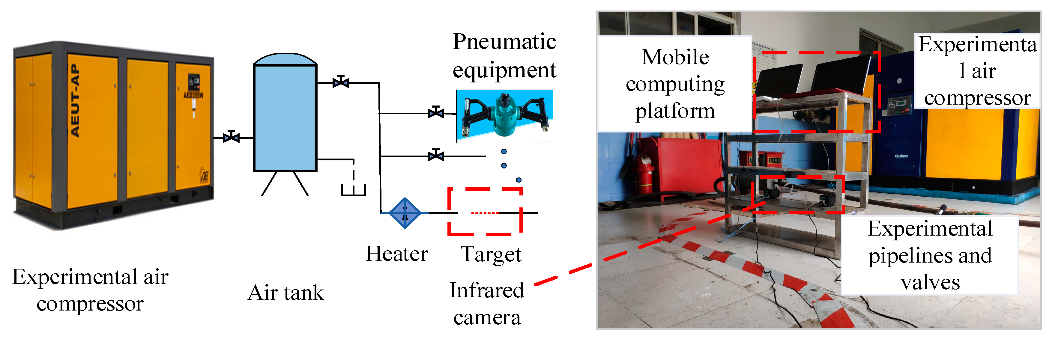
3.1. Experimental Platform Construction

In order to verify the feasibility and practicability of the air compressor pipeline leak identification system, an experimental system is built in the air compressor room of Sanmenxia Longwangzhuang Coal Industry Co., Ltd. The tests are conducted on five working conditions, including normal pipeline, leaking pipeline, worn pipeline, normal valve and leaking valve. The layout of the test bench is shown in Figure 6 and the captured infrared images are shown in the Figure 7.

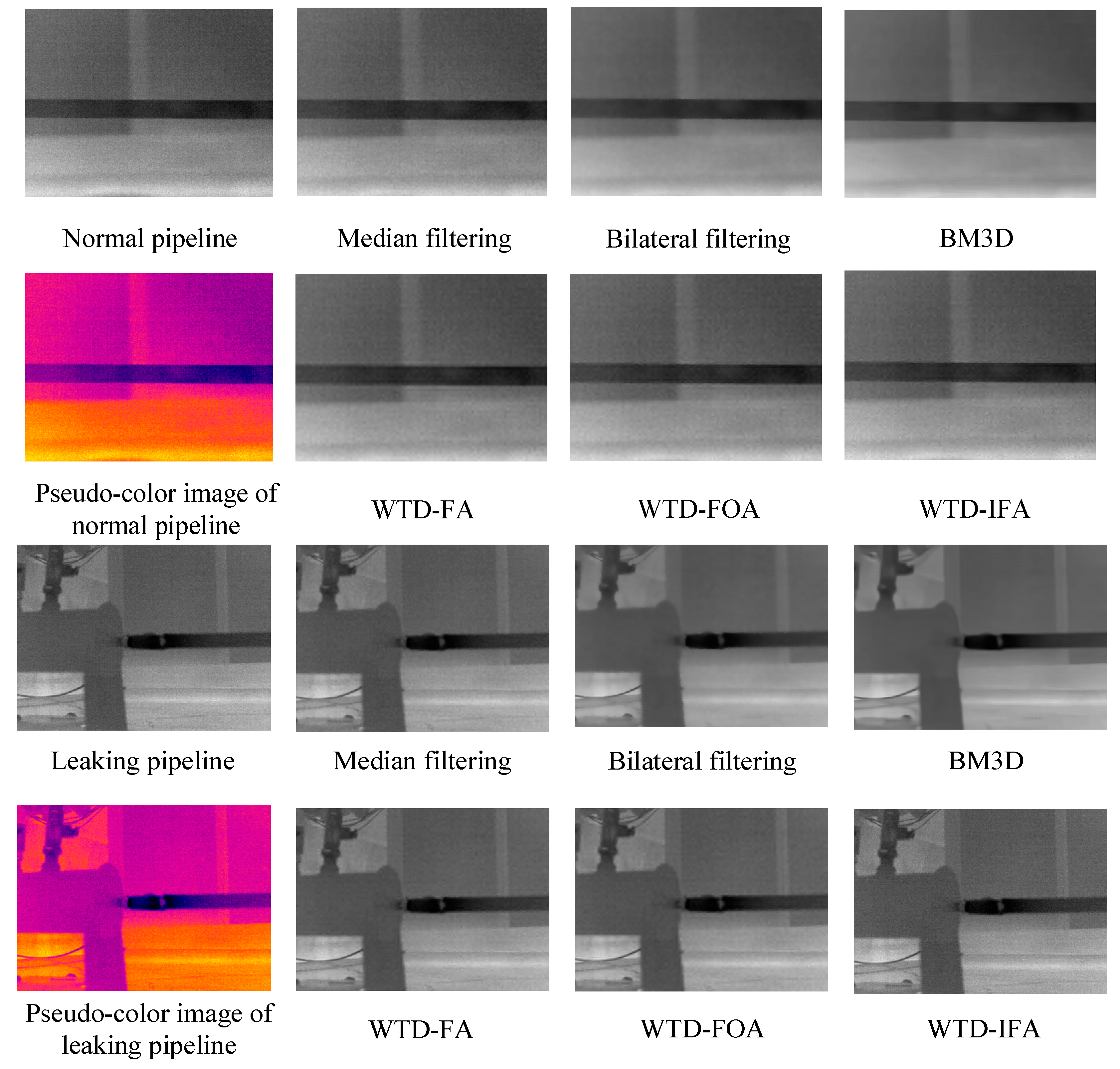
3.2. Infrared Image Denoising Experiments

The configuration and parameters of the processing platform of the identification system are shown in Table 4, and the model and main parameters of the infrared camera are shown in

Table 5. Parameters of online thermal imaging camera.

Type	Parameter
Infrared camera brand Detector type	Juge Electronics Uncooled focal plane
Wavelength range	7.5–14 μm
Pixels	384 × 288
Frame rate	50 Hz
Operating temperature	−30~60 °C
Temperature measurement range	0–300 °C
Temperature measurement accuracy	2 °C
focal length	10 mm
Angle of view	37.4° × 28°
Angular resolution	1.7 mrad

.

The WTD-IFA algorithm and the remaining five different denoising algorithms are used to denoise the infrared image and denoising results are shown in Figure 8, where FOA refers to fruit fly optimization algorithm. In order to evaluate the denoising effect more objectively, the information entropy of the image and the energy gradient function of the image are used as evaluation indicators. The information entropy of the image is a feature statistical form, which reflects the average amount of information in the image, so the entropy can be used as a focus evaluation standard. In general, the higher the entropy is, the clearer the image will be. The energy gradient of the image accumulates all pixel gradient values as definition evaluation values, so the larger the energy gradient value is, the clearer the image will be. The results of the denoising evaluation are shown in

Table 6. Information entropy of denoising images.

	Parameter	Image Information Entropy
Method		Normal Pipeline	Leaking Pipeline	Worn Pipeline	Normal Valve	Leaking Valve
Noisy image		6.70	6.39	6.56	5.99	6.53
Median filtering		6.55	6.25	6.42	5.82	6.39
Bilateral filtering		7.04	6.76	6.98	6.33	6.87
BM3D		7.92	7.69	7.88	7.34	7.77
WTD-FA		7.08	6.82	7.02	6.38	6.92
WTD-FOA		7.08	6.82	7.03	6.38	6.91
WTD-IFA		7.10	6.83	7.04	6.39	6.92

and

Table 7. Energy gradient of denoising images.

	Parameter	Image Information Entropy
Method		Normal Pipeline	Leaking Pipeline	Worn Pipeline	Normal Valve	Leaking Valve
Noisy image		20.37	21.18	20.02	21.91	21.21
Median filtering		22.96	22.81	22.74	23.86	22.95
Bilateral filtering		25.84	24.91	25.59	25.67	24.67
BM3D		26.34	25.95	26.00	25.84	25.84
WTD-FA		24.04	23.39	23.97	23.96	23.52
WTD-FOA		23.99	23.35	23.90	24.33	23.45
WTD-IFA		25.44	24.26	24.15	24.44	24.20

.

It can be seen from Table 6 that the Block-Matching 3-Dimension (BM3D) algorithm obtains the maximum entropy value of image information, and the WTD-IFA proposed in this paper is closely followed by it, with suboptimal results. The median filtering algorithm causes the information entropy of the image to drop, the remaining algorithms increase the information entropy of the image. The denoising effects of the three adaptive algorithms based on wavelet threshold are similar, and the improved WTD-IFA algorithm in this paper can achieve better results.

Another evaluation index selected in this paper is the energy gradient function of the image and the comparison results are shown in Table 7. The top three algorithms are BM3D, bilateral filtering and the algorithm proposed in this paper, and the image energy gradient of the three algorithms is obviously superior to other algorithms. The denoising effect of the bilateral filtering algorithm is similar to that of the three adaptive algorithms based on the wavelet threshold. The median filtering with the poor denoising effect cannot meet the system requirements. In contrast, the BM3D algorithm has the best denoising effect.

In order to better prove the superiority of the algorithm, this paper records the processing time of the algorithm mentioned, as shown in

Table 8. Denoising time of infrared images.

	Parameter	Image Information Entropy
Method		Normal Pipeline	Leaking Pipeline	Worn Pipeline	Normal Valve	Leaking Valve
Median filtering		1.0989	1.0479	1.0426	1.0575	1.0632
Bilateral filtering		1.8838	2.0553	2.1209	2.0259	2.2391
BM3D		14.7613	17.3301	17.3533	15.0779	17.3111
WTD-FA		1.0848	1.1081	1.2193	1.1766	1.2209
WTD-FOA		1.1856	1.2467	1.2375	1.2531	1.2738
WTD-IFA		1.0839	1.1192	1.1205	1.1784	1.3218

. Combined with the results of Table 6 and Table 7, it is concluded that BM3D algorithm has obtained the optimal results in terms of information entropy and energy gradient, but its processing time is longer. The algorithm proposed in this paper has the same processing time as other algorithms, and has achieved excellent results in the indicators of information entropy and gradient, which is more competitive than other comparison algorithms in solving image denoising problems.

In summary, the WTD-IFA algorithm proposed in this paper has a good denoising effect and a fast running speed, which can meet the requirements of pipeline compressor air leak identification systems.

3.3. SVM Classification Experiment Results

In order to verify the effectiveness of the proposed method, infrared images in the five working conditions of the normal pipeline, leaking pipeline, worn pipeline, normal value and leaking valve are collected, respectively. In each working conditions, 180 frame infrared images were selected to be used as SVM training samples, and 120 frame infrared images were selected to be used as SVM test samples. In addition, the genetic algorithm [31,32], particle swarm optimization [33,34] and IFA are used to optimize the two key SVM parameters of the penalty factor C and radial basis kernel function $\Upsilon$ to verify the optimization performance of IFA. The classification recognition results are shown in

Table 9. Genetic algorithm optimization classification confusion matrix.

	Prediction	Normal Pipeline	Leaking Pipeline	Worn Pipeline	Normal Valve	Leaking Valve
Reality
Normal pipeline		19	0	1	0	0
Leaking pipeline		1	15	4	0	0
Worn pipeline		0	1	19	0	0
Normal valve		0	0	0	20	0
Leaking valve		0	0	0	2	18

,

Table 10. Particle swarm algorithm optimization classification confusion matrix.

	Prediction	Normal Pipeline	Leaking Pipeline	Worn Pipeline	Normal Valve	Leaking Valve
Reality
Normal pipeline		19	0	1	0	0
Leaking pipeline		0	17	3	0	0
Worn pipeline		0	2	18	0	0
Normal valve		0	0	0	20	0
Leaking valve		0	0	0	1	19

,

Table 11. IFA optimization classification confusion matrix.

	Prediction	Normal Pipeline	Leaking Pipeline	Worn Pipeline	Normal Valve	Leaking Valve
Reality
Normal pipeline		20	0	0	0	0
Leaking pipeline		0	18	2	0	0
Worn pipeline		0	1	19	0	0
Normal valve		0	0	0	20	0
Leaking valve		0	0	0	1	19

and

Table 12. Overall recognition results based on SVM with different algorithms.

Intelligent Algorithm	Image Classification Prediction Accuracy	Single Image Processing Average Time
Genetic algorithm	91.00%	2.2068
Particle swarm optimization	93.00%	2.5009
IFA	96.00%	2.3518

.

It can be seen from the Table 9, Table 10, Table 11 and Table 12 that the infrared image is easy to be confused under the two working conditions of leakage pipeline and worn pipeline and the image of the leaking valve is easily erroneously recognized as a normal valve image. In the comparison of the above three optimization algorithms, the support vector machine optimized by IFA has the highest classification accuracy of 96.00%, and the average processing classification time of a single image is 2.35 s, which can meet the recognition requirements of the system.

4. Conclusions

In this paper, a novel intelligent diagnosis method based on the integration of IFA, the adaptive wavelet threshold denoising algorithm, Otsu-Grabcut image segmentation algorithm, HOG-GLCM feature extraction algorithm and SVM is proposed to recognize the leak state of a compressor pipeline. In the proposed method, an improved FA is designed to optimize the parameters of the WTD algorithm and SVM, respectively. The obtained WTD-IFA is used to denoise the infrared images, the Otsu-Grabcut algorithm is introduced to segment the images, and the HOG-GLCM is utilized to achieve feature extraction. Then, an optimal SVM classifier is constructed to produce the intelligent diagnosis of pipeline leak. In order to evaluate the effectiveness of the proposed method, an experimental system is built and the images under five different working conditions are collected. Some simulations and experiments are provided. The results indicate that the WTD algorithm based on IFA has a better denoising effect on infrared images. The average recognition accuracy of SVM with IFA can reach up to 96% and the results verify the feasibility and superiority of the proposed method.

References

1. Bao, C.; Yang, C. Remote On-line Monitoring System for Air Compressor Used for Mine Based on Configuration Technology. Coal Mine Mach. 2012, 7, 236–238. [Google Scholar]
2. Jian-zhang, L.U. Compressed Air Self Rescue System in Underground Mine. Coal Sci. Technol. 2010, 12, 4–6. [Google Scholar]
3. Maolin, C. Modern Pneumatic Technology and Practice Lecture 10: Energy-Saving in Pneumatic System. Hydraul. Pneum. Seals 2008, 28, 59–63. [Google Scholar]
4. Šešlija, D.; Ignjatović, I.; Dudić, S.; Lagod, B. Potential energy savings in compressed air systems in Serbia. Afr. J. Bus. Manag. 2011, 5, 5637–5645. [Google Scholar]
5. Kreith, F.; Goswami, D.Y. Energy Management and Conservation Handbook; CRC Press: Boca Raton, FL, USA, 2007. [Google Scholar]
6. Madding, R.; Benson, R. Detecting SF6 insulating gas leaks with an IR imaging camera. Electr. Today 2007, 19, 9–15. [Google Scholar]
7. Dudić, S.; Ignjatović, I.; Šešlija, D.; Blagojević, V.; Stojiljković, M. Leakage quantification of compressed air using ultrasound and infrared thermography. Measurement 2012, 45, 1689–1694. [Google Scholar] [CrossRef]
8. Meng, L.; Yuxing, L.; Wuchang, W.; Juntao, F. Experimental study on leak detection and location for gas pipeline based on acoustic method. J. Loss Prev. Proc. 2012, 25, 90–102. [Google Scholar] [CrossRef]
9. Chis, T. Pipeline leak detection techniques. Ann. Comput. Sci. 2009, 5, 25–34. [Google Scholar]
10. Wang, Y. Application and research of DSP in the portable air-leakage detector. Machinery 2005, 3, 56–59. [Google Scholar]
11. Jin, H.; Zhang, L.; Liang, W.; Ding, Q. Integrated leakage detection and localization model for gas pipelines based on the acoustic wave method. J. Loss Prev. Proc. 2014, 27, 74–88. [Google Scholar] [CrossRef]
12. Salisbury, J.W.; D’Aria, D.M. Emissivity of terrestrial materials in the 8–14 μm atmospheric window. Remote Sens. Environ. 1992, 42, 83–106. [Google Scholar] [CrossRef]
13. Yang, X. Firefly algorithm. In Nature-Inspired Metaheuristic Algorithms; Elsevier: Amsterdam, The Netherlands, 2014; Volume 20, pp. 111–127. [Google Scholar]
14. Hassanzadeh, T.; Kanan, H.R. Fuzzy FA: A modified firefly algorithm. Appl. Artif. Intell. 2014, 28, 47–65. [Google Scholar] [CrossRef]
15. Haji, V.H.; Monje, C.A. Fractional-order PID control of a chopper-fed DC motor drive using a novel firefly algorithm with dynamic control mechanism. Soft Comput. 2018, 22, 6135–6146. [Google Scholar] [CrossRef]
16. Kumar, S.V.; Nagaraju, C. FFBF: Cluster-based Fuzzy Firefly Bayes Filter for noise identification and removal from grayscale images. Clust. Comput. 2019, 22, 1–23. [Google Scholar] [CrossRef]
17. Mo, Y.; Ma, Y.; Zheng, Q. Optimal choice of parameters for firefly algorithm. In 2013 Fourth International Conference on Digital Manufacturing and Automation; IEEE: Piscataway, NJ, USA, 2013; pp. 887–892. [Google Scholar]
18. Soto, C.; Valdez, F.; Castillo, O. A review of dynamic parameter adaptation methods for the firefly algorithm. In Nature-Inspired Design of Hybrid Intelligent Systems; Springer: Cham, Switzerland, 2017; pp. 285–295. [Google Scholar]
19. Liu, Q.; Jiang, Z.; Shi, H. Maximum Entropy Image Segmentation Method Based On Improved Firefly Algorithm. In Journal of Physics: Conference Series; IOP Publishing: Bristol, UK, 2019; p. 032023. [Google Scholar]
20. Hidalgopaniagua, A.; Vegarodriguez, M.A.; Ferruz, J.; Pavon, N. Solving the multi-objective path planning problem in mobile robotics with a firefly-based approach. Soft Comput. 2017, 4, 949–964. [Google Scholar] [CrossRef]
21. Sadhu, A.K.; Konar, A.; Bhattacharjee, T.; Das, S. Synergism of Firefly Algorithm and Q-Learning for Robot Arm Path Planning. Swarm Evol. Comput. 2018, 43, 50–68. [Google Scholar] [CrossRef]
22. Yang, X. Firefly algorithm, Levy flights and global optimization. In Research and Development in Intelligent Systems XXVI; Springer: London, UK, 2010; pp. 209–218. [Google Scholar]
23. Abdullah, A.; Deris, S.; Mohamad, M.S.; Hashim, S.Z.M. A new hybrid firefly algorithm for complex and nonlinear problem. In Distributed Computing and Artificial Intelligence; Springer: Berlin/Heidelberg, Germany, 2012; pp. 673–680. [Google Scholar]
24. Yang, Q.; Tan, K.; Ahuja, N. Real-time O (1) bilateral filtering. In 2009 IEEE Computer Society Conference on Computer Vision and Pattern Recognition; IEEE: Piscataway, NJ, USA, 2009; pp. 557–564. [Google Scholar]
25. Feruglio, P.F.; Vinegoni, C.; Gros, J.; Sbarbati, A.; Weissleder, R. Block matching 3D random noise filtering for absorption optical projection tomography. Phys. Med. Biol. 2010, 55, 5401–5415. [Google Scholar] [CrossRef] [Green Version]
26. Deng, G.; Liu, Z. A wavelet image denoising based on the new threshold function. In 2015 11th International Conference on Computational Intelligence and Security (CIS); IEEE: Piscataway, NJ, USA, 2015; pp. 158–161. [Google Scholar]
27. Otsu, N. A threshold selection method from gray-level histograms. IEEE Trans. Syst. Man Cybern. 1979, 9, 62–66. [Google Scholar] [CrossRef] [Green Version]
28. Rother, C.; Kolmogorov, V.; Blake, A. Interactive foreground extraction using iterated graph cuts. ACM Trans. Graph. 2004, 3, 309–314. [Google Scholar] [CrossRef]
29. Haralick, R.M.; Shanmugam, K.; Dinstein, I.H. Textural features for image classification. IEEE Trans. Syst. Man Cybern. 1973, 6, 610–621. [Google Scholar] [CrossRef] [Green Version]
30. Chen, J.; Yin, Y.; Han, L.; Zhao, F. Optimization Approaches for Parameters of SVM. In Proceedings of the 11th International Conference on Modelling, Identification and Control, Tianjin, China, 13–15 July 2019; Springer: Berlin/Heidelberg, Germany, 2020; pp. 575–583. [Google Scholar]
31. Maulik, U.; Bandyopadhyay, S. Genetic algorithm-based clustering technique. Pattern Recogn. 2000, 33, 1455–1465. [Google Scholar] [CrossRef]
32. Demidova, L.A.; Egin, M.M.; Tishkin, R.V. A Self-tuning Multiobjective Genetic Algorithm with Application in the SVM Classification. Procedia Comput. Sci. 2019, 150, 503–510. [Google Scholar] [CrossRef]
33. Zhou, C.; Gao, H.B.; Gao, L.; Zhang, W. Particle Swarm Optimization (PSO) Algorithm. Appl. Res. Comput. 2003, 12, 7–11. [Google Scholar]
34. Raj, S.; Ray, K.C. ECG Signal Analysis Using DCT-Based DOST and PSO Optimized SVM. IEEE Trans. Instrum. Meas. 2017, 66, 470–478. [Google Scholar] [CrossRef]
Figure 1. Improved firefly algorithm flow.
Applsci 10 05991 g001
Figure 2. Iteration curves for the improved firefly algorithm (IFA), Levy-flight Firefly Algorithm (LFA), firefly algorithm (FA): (a) Iterative curve of function f1; (b) Iterative curve of function f2; (c) Iterative curve of function f3; (d) Iterative curve of function f4; (e) Iterative curve of function f5; (f) Iterative curve of function f6; (g) Iterative curve of function f7; (h) Iterative curve of function f8.
Applsci 10 05991 g002aApplsci 10 05991 g002b
Figure 3. Flowchart of the wavelet threshold infrared image denoising algorithm (WTD-IFA) algorithm.
Applsci 10 05991 g003
Figure 4. The image segmentation result.
Applsci 10 05991 g004
Figure 5. The recognition process of the proposed method.
Applsci 10 05991 g005
Figure 6. Pipeline leak experiment platform for mine air compressor.
Applsci 10 05991 g006
Figure 7. Infrared images of five working conditions.
Applsci 10 05991 g007
Figure 8. Image denoising results based on different algorithms.
Applsci 10 05991 g008aApplsci 10 05991 g008b