Handwritten Digit Recognition: Hyperparameters-Based Analysis

Abstract

Neural networks have several useful applications in machine learning. However, benefiting from the neural-network architecture can be tricky in some instances due to the large number of parameters that can influence performance. In general, given a particular dataset, a data scientist cannot do much to improve the efficiency of the model. However, by tuning certain hyperparameters, the model’s accuracy and time of execution can be improved. Hence, it is of utmost importance to select the optimal values of hyperparameters. Choosing the optimal values of hyperparameters requires experience and mastery of the machine learning paradigm. In this paper, neural network-based architectures are tested based on altering the values of hyperparameters for handwritten-based digit recognition. Various neural network-based models are used to analyze different aspects of the same, primarily accuracy based on hyperparameter values. The extensive experimentation setup in this article should, therefore, provide the most accurate and time-efficient solution models. Such an evaluation will help in selecting the optimized values of hyperparameters for similar tasks.

1. Introduction

For computer scientists, the complexity of recognizing handwriting is becoming increasing demanding due to a significant variation in languages. The problem remains even if the variable of language is kept constant, by categorizing handwriting by similar languages. Every piece of writing is different, though there are some similarities that can be classified together. The task for a data scientist, in this case, is to group the digits involved in writing a similar language in categories that would indicate related groups of the same numbers or characters. The optimization of this process is of utmost importance, as one wants to recognize handwriting as it is written. The classifiers that are used in these cases vary in their methods and recognition speeds, along with the accuracy of recognition.

Neural networks (NN) have proved useful in a vast range of fields, classification being one of the most basic. NNs show excellent performance for the classification of images by extracting features from images and making predictions based on those features. Many different types of NN scans be used for classification, i.e., convolutional neural networks (CNN), recurrent neural networks (RNN), etc. Each type has its architecture, but some properties remain the same. As each layer consists of neurons, each neuron is assigned weight and activation functions. First, we will look at the architecture of each neural network.

1.1. Convolution Neural Network (CNN)

Convolutional neural networks (CNNs) have passed through many stages to attain the level of performance recognized in today’s era. Fukushima et al. [1] first presented Neocognition, capable of extracting features from images in 1983. After a few variants in 1989, LeCun et al. [2] proposed a network for character recognition. CNNs are the most important deep-learning algorithms and are widely used in image recognition, object detection, face recognition, etc. CNN works on the principle of multiple convolutions from which it derives its architecture [3].

CNN works by a series of different layer to extract the features from images:

(1)

Convolutional;

(2)

Pooling;

(3)

Flatten;

(4)

Fully connected layer.

However, 1 and 2 can be repeated multiple times to help increase learning from the abstract feature.

(1)

Convolutional first takes in input and then extract features from it. It conserves pixel relationships by learning from them, using a series of small squares. A computation is a mathematical operation between the filter and the part of the image under consideration. This filter performs various functions such as edge detection, blurring and sharpening the image.

(2)

The pooling layer downsamples the images when they are too large. This helps retain important features while reducing image size. The most crucial pooling type is Spatial pooling, also called subsampling or downsampling, which reduces the dimension of the image by retaining essential features. Pooling is further categorized as follows:

(a)

Max pooling;

(b)

Average pooling;

(c)

Sum pooling.

(3)

Flatten(ing) flats all the values into a single dimension tensor obtained from the pooling layer. The dense layer and connected layer follow this layer.

(4)

The fully connected layer is the dense feed-forward neural network. These layers are fully connected with the flatten layers.

1.2. Recurrent Neural Network

The term recurrent neural networks was first coined by Pearlmutter [4] in 1989, where he explained the learning process of RNN for state space trajectories. Recurrent neural networks (RNN) are part of an Artificial neural network, which, unlike a feedforward neural network, can retain essential features about the past and has a memory unit in it [5]. Basic feedforward also can remember, but it only retains training information. Whereas RNN retains training information, it can also learn from every input(s) while generating output(s).

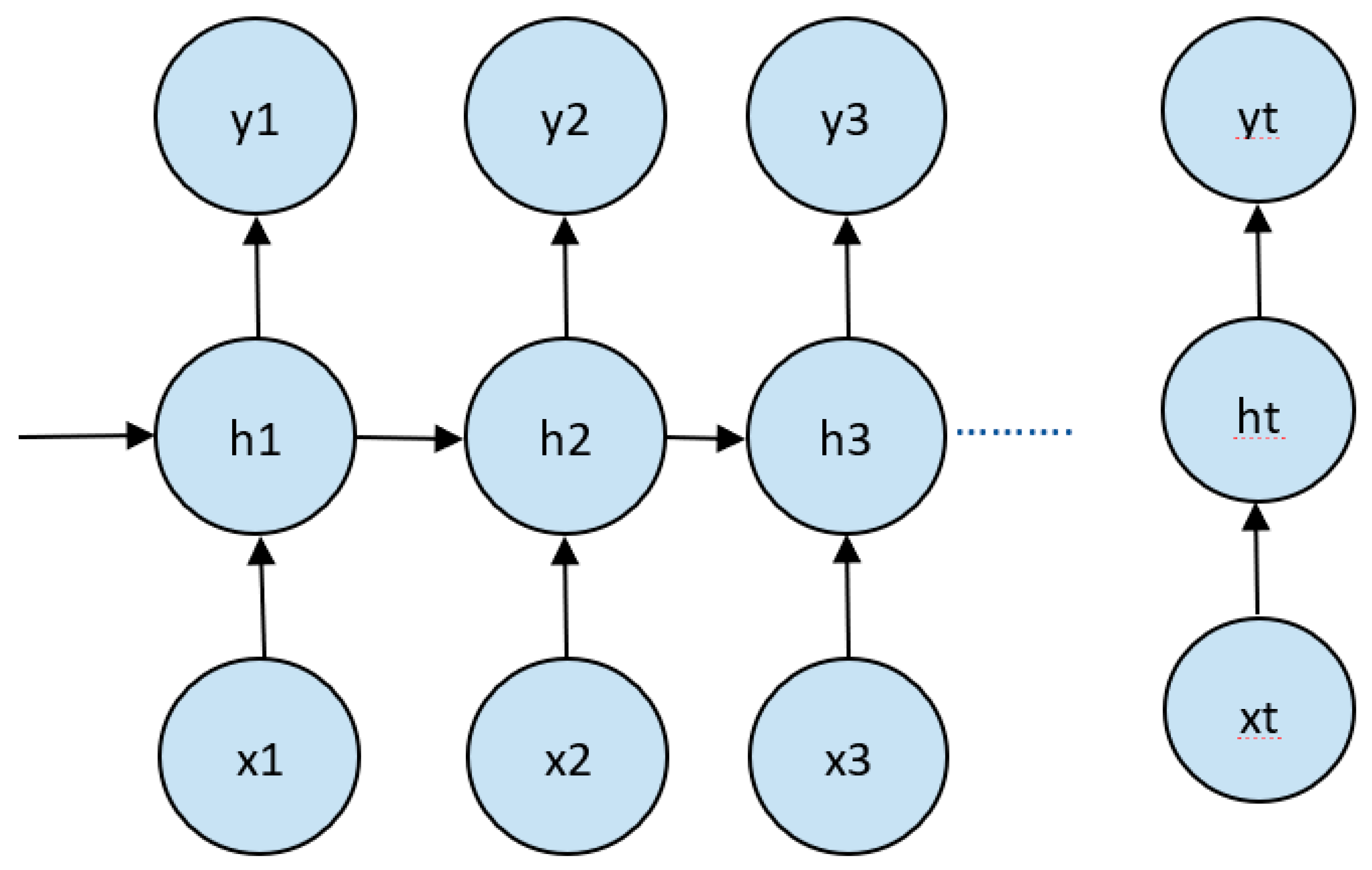
RNN can take one or more input(s) data and generate one or more output(s). These output(s) are not only affected by the input data alone, but also by the hidden state vector, which remembers the output generated by the input. Accordingly, a sample input can give a different output based on the previous input data inside the series.

The basic architecture of RNN is shown in Figure 1. In this figure, y1, y2 and y3 are the outputs generated from the x1, x2 and x3 nodes, and h is hidden state.

1.3. Multi Layer Perceptron (MLP)

MLPs are nothing, but neural network in classical form. It is a form of the feed-forward neural networks. It consists of at least three layers, an input layer, a hidden layer and an output layer. The layers of neural networks are stacked upon each other; they are called hidden layers [6]. Since a neural network must be nonlinear, activation like ReLU is used to add nonlinearities in the layer [7].

1.4. Siamese Neural Network

Chopra et al. [8] gave the idea of Siamese neural networks in 2005. A Siamese NN is part of an artificial neural network which has two or more identical subnetworks. These subnetworks are assigned the same weights and outputs, and any parameter update is mirrored across both networks. Since these subnetworks are similar, they have only a few parameters to compute and are faster than the other networks [9]. Siamese NN can be used for checking the identity of two documents—photographs and images—and are widely used.

1.5. Knowledge-Transfer Model

Transfer learning or knowledge-transfer modeling is an approach in which previously trained offline models are augmented to new similar problems. A base network is first trained for a standard dataset. The trained model is then augmented with the latest models needed in preparation for a specific task. In most cases, this helps in enhancing accuracy and reducing the training and execution times of the new models.

1.6. Hyper Parameters

While defining the structure of a NN, the factors that matter most are the hyperparameters. If neglected and not selected properly, they can be the cause of high error, resulting in wrong predictions [10]. We deal with the following parameters:

(1)

Learning rate dynamics: learning rate is a crucial factor in machine learning, determining the extent to which new data may be changed by considering old data. Here the data predominantly signify the weight. When the learning rate is considerably high, it may jump or escape the minima and converge fast. This causes low accuracy and the model to be unfit. Similarly, without the lower learning rate, the model takes much time to converge and get stuck in undesirable local minima. This increases the model’s compilation time and sometimes leads to overfitting. Deep learning training generally relies on training, using the stochastic gradient descent method. The stochastic gradient descent (SGD) approach updates the parameters after each example. Batch gradient descent (BGD) updates parameters after processing a batch. This hastens the stochastic descent when the training set is extensive. This updating of weight is done by the most significant algorithm known as the back-propagation algorithm. This optimization algorithm has many hyperparameters, and the learning rate is one.

(2)

Momentum dynamics: In the stochastic gradient descent optimization algorithm, weights are updated after every iteration. This is efficient when the dataset is quite large, but sometimes this progression is not that fast. To accelerate the learning process, momentum will smooth the progression, thereby reducing training time. We try to adapt the rate by varying the momentum in the SGD parameter and fixing the learning rate. Furthermore, we check model performance and accuracy.

(3)

Learning rate (α) decay: As discussed earlier, SGD is an excellent optimization algorithm. In SGD, an important hyperparameter called the decay rate is used. Decay causes the learning rate to be reduced over every iteration, making the learning rate less than the previous algorithm. Generally, the decay rate is computed as follows:

$${\alpha }_{new}={\alpha }_{old}\times \frac{1}{\left(decay\times iteration\right)}$$

(1)

where $\alpha$ is known as the learning rate.

(4)

Drop learning rate on plateau: This parameter constantly monitors the metric, and if the metric does not change over given epochs, it drops the learning rate. We continued by exploring different values for the “patience” which checks how many epochs wait to monitor the change and then drops the new learning rate. This learning rate is usually lower than the previous learning rate. For this experiment, we are using a constant learning rate of 0.01 and then drop the learning rate by a factor set to the value of 0.1. These values can be tuned for better performance.

(5)

Adaptive learning rates: We know the learning decay rate is very critical and hard to implement; there is no hard and fast rule to get the best values. To deal with this, previously best-known algorithms are used for the learning rate, as follows:

(a)

Adaptive gradient algorithm (AdaGrad);

(b)

Root mean square propagation (RMSprop);

(c)

Adaptive moment estimation (Adam).

All employ a different methodology and use various approaches. Again, the optimization algorithm has its drawbacks and tradeoffs: no algorithm is perfect. We use these algorithms to find the better one and accordingly use them for our metric calculation.

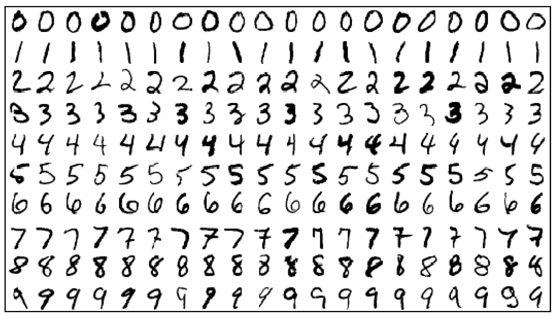
In this paper, we compare the five neural networks described above for the classification of the MNIST dataset [11]. Then we check the alteration in accuracy and execution time by changing the hyperparameters described above. The MNIST database is compiled by the National Institute of Standard and Technology. The database comprises 70,000 images of handwritten digits. These in turn are divided into 60,000 for training and 10,000 for testing. The dimension for each image is 28 × 28 (784 pixels). We used MNIST because it is concise and can be easily used. Figure 2 shows a sample of images in the MNIST dataset. The algorithms work at different magnitudes and tend to sublimate each other completely. However, the potential for comparison is still there. Simultaneously, each of these algorithms has its strengths and weaknesses, which is relevant to comparing them all in a single task and elaborating their significant suitability for accuracy and speed. This makes for comparable potential, along with being able to reach the desired target.

As a consequence, our primary contributions are as follows:

• A comprehensive evaluation of neural network-based architectures for handwritten digit recognition.
• An investigation of the hyperparameters of neural network-based architectures for improving the accuracy of handwritten digit recognition.

2. Previous Work

There has been much work in the field of classification, especially for MNIST datasets. Many types of neural networks have been used for this purpose, and sometimes a combination of different algorithms has been used. Many new advanced forms of underlying neural networks were also tested on MNIST data.

Kessab et al. [12] used a multilayer perceptron (MLP) for the recognition of handwritten letters to build an optical character recognition (OCR) system. Koch et al. [13] used Siamese neural networks for one-shot image recognition, i.e., only one image of each class is used. Shuai et al. [14] built the Independently recurrent neural network (IndRNN), an advanced form of RNN and tested its performance on MNIST datasets. Chen et al. [15] built a probabilistic Siamese network and tested it on MNIST data. Chen used CNN for the image classification of MNIST [16].

Niu et al. [17] combined CNN with a support vector machine (SVM), a different approach for MNIST data classification. Similar work is done by Agarap et al. [18] combined CNN and SVM for image classification. Zhang et al. [19] combined SVM and k-nearest neighbors (KNN) for image classification. Vlontzos [20] used Random neural networks with extreme learning machines (ELM) to build a classifier that does not require large training datasets.

As it is an era that revolves around deep learning, many works have been done in hyperparameter tuning. Mostly, hyperparameters are selected through grid search; but there are many algorithms now that can tune them for better results. Loshchilov et al. [21] proposed covariance matrix adaptation evolution strategy (CMA-ES) for hyperparameter optimization. Smith et al. [22] proposed a disciplined approach for tuning the learning rate, batch size, momentum and weight decay. Domhan et al. [23] extrapolated the learning curves to speed up automatic hyperparameter optimization of deep neural networks. Bardenet et al. [24] merged optimization techniques with surrogate-based ranking for surrogate-based collaborative tuning (SCoT). They verified SCoT in two different experiments that outperformed standard tuning methods, but their approach is still suffering from limited meta-features. Koutsoukas et al. [25] studied the comparison between hyperparameters for modeling bioactivity data.

As seen from the above references, much work exists in the field of classification. No work has been done on a comparison between different neural networks based on changing hyperparameters. There are several givens in this paper:

• Results for efficiency of each neural network (NN) based on different hyperparameters;
• The best results of a comparison of different NNs based on hyperparameters selected after testing;
• Best model and hyperparameter values are given.

With the advent of deep learning, there has been more focus on developing techniques for recognition of handwritten letters and digits, using deep neural networks instead of hand-engineered features. The literature review of methods to classify and test handwritten data, using deep-learning techniques, is summarized in

Table 1. Comparison table of previous methodologies.

Reference	Methodology	Findings	Gaps Identified
Kessab et al. (2004) [12]	Applied MLP	MLP can be used for text recognition	There has been much work done in the field, but no comparison between neural networks on the basis of hyperparameter values.
Koch et al. (2015) [13]	Used Siamese neural networks for one-shot image recognition	One image can be used for classification of a single class
Li et al. (2018) [14]	Built IndRNN	IndRNN performs better than RNN and fills the gaps in RNN
Liu et al. (2013) [15]	Built probabilistic Siamese network	tested efficiency on MNIST dataset Classified MNIST
Niu et al. (2012) [17]	Combined CNN and SVM for classification	Classified MNIST
Agarap et al. (2017) [18]	Combined CNN and SVM for classification	Classified MNIST
Berg et al. (2006) [19]	Combined CNN and SVM	Performed image classification
Rastegari et al. (2016) [26]	Gave binary-weight-networks and XNOR-Networks	Updated CNN
Dutta et al. (2018) [27]	Made a hybrid improving architecture between CNN and RNN	Performs better than RNN on audio Synthesis and machine translation
Loshchilov et al. (2016) [21]	Used covariance matrix adaptation evolution strategy (CMA-ES)	Performed hyperparameter tuning
Smith et al. (2018) [22]	Worked with hyperparameters tuning	Optimized learning rate, batch size, momentum and weight decay
Domhan et al. (2015) [23]	Extrapolated the learning curves	Speeding up automatic hyperparameter optimization of deep neural networks
Bardenet et al. (2013) [24]	Used optimization techniques with surrogate-based ranking for surrogate-based collaborative tuning (SCoT)	Achieves standard tuning methods and single-problem surrogate-based optimization
Koutsoukas et al. (2017) [25]	Studied the comparison between hyperparameters	Modeling bioactivity data
Li et al. (2018) [28]	Proposed ASHA	Performs massive parallel hyperparameter tuning
Shang et al. (2020) [29]	Performed hyperparameter tuning	As an instance of best-arm identification in infinitely many-armed bandits

. This section gives a basic overview of work in the field to support our work, whereas the next section describes the methodology taken to prove our claims.

The rest of the paper is divided as follows: Section 3 describes the methodology, pipeline and experimental environment used. Section 4 will describe and analyze the results, on the basis of which the optimal hyperparameter values will be selected. In the end, Section 5 will conclude the study with some suggestions for future work.

3. Methodology

We used five neural networks for comparison purposes: CNN, RNN, multilayer perceptron, the Siamese model and the knowledge-transfer model. The hyperparameters tuned for each classification algorithm are: learning rate dynamics, momentum dynamics, learning rate Decay, Drop learning rate on the plateau and adaptive learning rates.

Each hyperparameter was changed to check the accuracy and execution time of the models and their effects.

Table 2. Hyperparameters values.

Hyperparameters	Values
Learning rate dynamics	1 × 10−0, 1 × 10−1, 1 × 10−2, 1 × 10−3, 1 × 10−4, 1 × 10−5, 1 × 10−6, 1 × 10−7
Momentum dynamics	0.0, 0.5, 0.9, 0.99
Learning rate Decay	1 × 10−1, 1 × 10−2, 1 × 10−3, 1 × 10−4
Drop learning rate on plateau	2, 4, 8, 10
adaptive learning rate	SGD, AdaGrad, RMSprop, Adam

shows the different values of hyperparameters taken for testing the models. The dataset used for checking the performances is the MNIST dataset.

3.1. Preprocessing of Data

The MNIST dataset has the dimensions of 28 × 28 (784 pixels). All the images are of the same size; hence we did not proceed with generalizations. The images are split into two sets: x_train and y_train as the training set and x_test and y_test as the testing set. The selection of hyperparameter values was selected through the accuracy obtained by the test set. The images are normalized by dividing each image by 255 steps. Each channel is 8 bits and when we split it, the value is confined between 0–1. This makes it precise and computationally efficient based on the following equation:

$$X_{normalized}=\frac{X-X_{min}}{X_{max}-X_{min}}$$

(2)

3.2. Architecture of Models

The models will be trained through training sets and selection of hyperparameter values will be done on the basis of accuracy obtained by testing the models on test sets. The factors for measuring performance are:

(1)

Test loss

(2)

Test accuracy

(3)

Execution time

The architecture of CNN, RNN and MLP is shown in

Table 3. Convolutional neural network (CNN) architecture.

Type	Filters	Kernel	Function	Output
Convolutional	32	3 × 3	Relu	(26, 26, 32)
Convolutional	64	3 × 3	Relu	(24, 24, 64)
Max-pooling	–	2 × 2	–	(12, 12, 64)
Dropout (0.25)	–	–	–	(12, 12, 64)
Flatten	–	–	–	9216
Dense	–	–	Relu	128
Dropout (0.5)	–	–	–	128
Dense	–	–	Softmax	10

,

Table 4. Recurrent neural network (RNN) architecture.

Type	Function	Output
Simple RNN	–	50
Dense	–	10
Activation	Softmax	10

and

Table 5. Multilayer perceptron (MLP) architecture.

Type	Function	Output
Dense	Relu	512
Dropout (0.2)	–	512
Dense	Relu	512
Dropout (0.2)	–	512
Dense	Sofgtmax	10

, respectively. The base model is shown in

Table 6. Base models for Siamese networks.

Type	Function	Output
Dense	Relu	128
Dropout (0.1)	–	128
Dense	Relu	128
Dropout (0.1)	–	128
Dense	Relu	128

. This model is used as two branches of the Siamese Network.

Table 7. Architecture of base and knowledge-transfer model.

Type	Filters	Kernel	Function	Output
convolutional	32	3 × 3	–	(26, 26, 32)
Activation	–	–	Relu	(26, 26, 32)
convolutional	32	3 × 3	–	(24, 24, 32)
Activation	–	–	Relu	(24, 24, 32)
Max-pooling	–	2 × 2	–	(12, 12, 32)
Dropout (0.25)	–	–	–	(12, 12, 32)
Flatten	–	–	–	4608
Dense	–	–	–	128
Activation	–	–	Relu	128
Dropout (0.5)	–	–	–	128
Dense	–	–	–	5
Activation	–	–	Softmax	5

shows the architecture of the model used for transfer knowledge. The model was first trained for 5 digits from 1 to 5. Then feature layers were frozen and the model was trained for 5 digits 6 to 10. The number of trainable features in base models is 600,165 while in the knowledge-transfer model the number of trainable features is 590,597. It can be seen that each model is defined in table according to all the parameters that were kept constant throughout experiment.

In these networks, we changed the values of all the hyperparameters one-by-one, i.e., we started from the first value of each parameter in Table 2 and changed the value of the learning rate first while keeping other parameters constant and measuring performance. Then we set the learning rate at which the performance was maximum and changed the value of momentum dynamics. This process was repeated for all hyperparameter values and for each model. For each parameter value, the Network was observed for 10 epochs or until it converged. After the values of all the parameters was monitored, a conclusion was drawn as described in the result section.

4. Results

We performed a rigorous experiment while checking all hyperparameters. We experimented extensively and tested with the Google Colab with a constant epoch = 10 for all of them.

4.1. Testing on CNN

First, we tested the CNN model. The results are shown in

Table 8. Effect of learning rate on CNN.

Learning Rate	Execution Time (s)	Test Loss	Test Accuracy
1.0	158.6201	14.534	0.098
0.1	187.0275	14.490	0.101
0.01	193.6009	0.008	0.097
0.001	195.7196	0.150	0.975
1 × 10−5	189.0192	0.002	0.900
1 × 10−6	182.1515	0.003	0.700
1 × 10−7	186.0239	10.008	0.220

. We conclude from this table that choosing the learning rate = 0.001 will yield the highest accuracy, but with the tradeoff of the highest execution time. Then we changed the momentum for CNN. The results are shown in

Table 9. Effect of momentum on CNN.

Momentum	Execution Time (s)	Test Loss	Test Accuracy
0.0	191.0786	14.4917	0.1009
0.5	183.0671	14.4917	0.1009
0.9	189.7915	14.4611	0.1028
0.99	188.8871	14.5175	0.0993

. We see that momentum does not exhibit in the model performance boost, and thereby tuning it will be of no use and a waste of computational power and time. After this, we changed learning rate decay. The results are shown in

Table 10. Effect of learning rate decay on CNN.

Decay Rate	Execution Time (s)	Test Loss	Test Accuracy
1 × 10−1	191.9412	14.491	0.1009
1 × 10−2	189.7679	0.1009	0.9517
1 × 10−3	189.9171	0.0467	0.9839
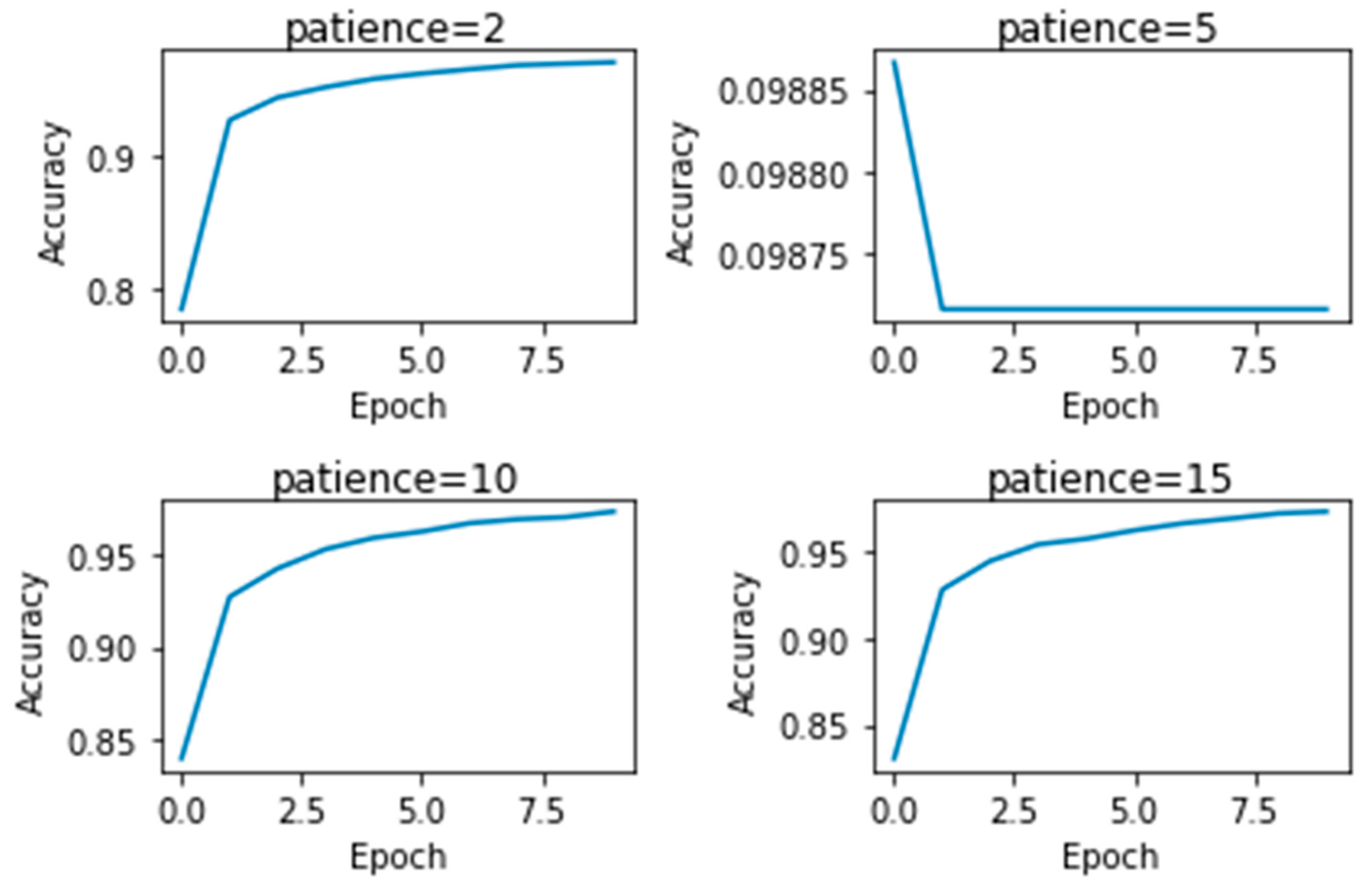
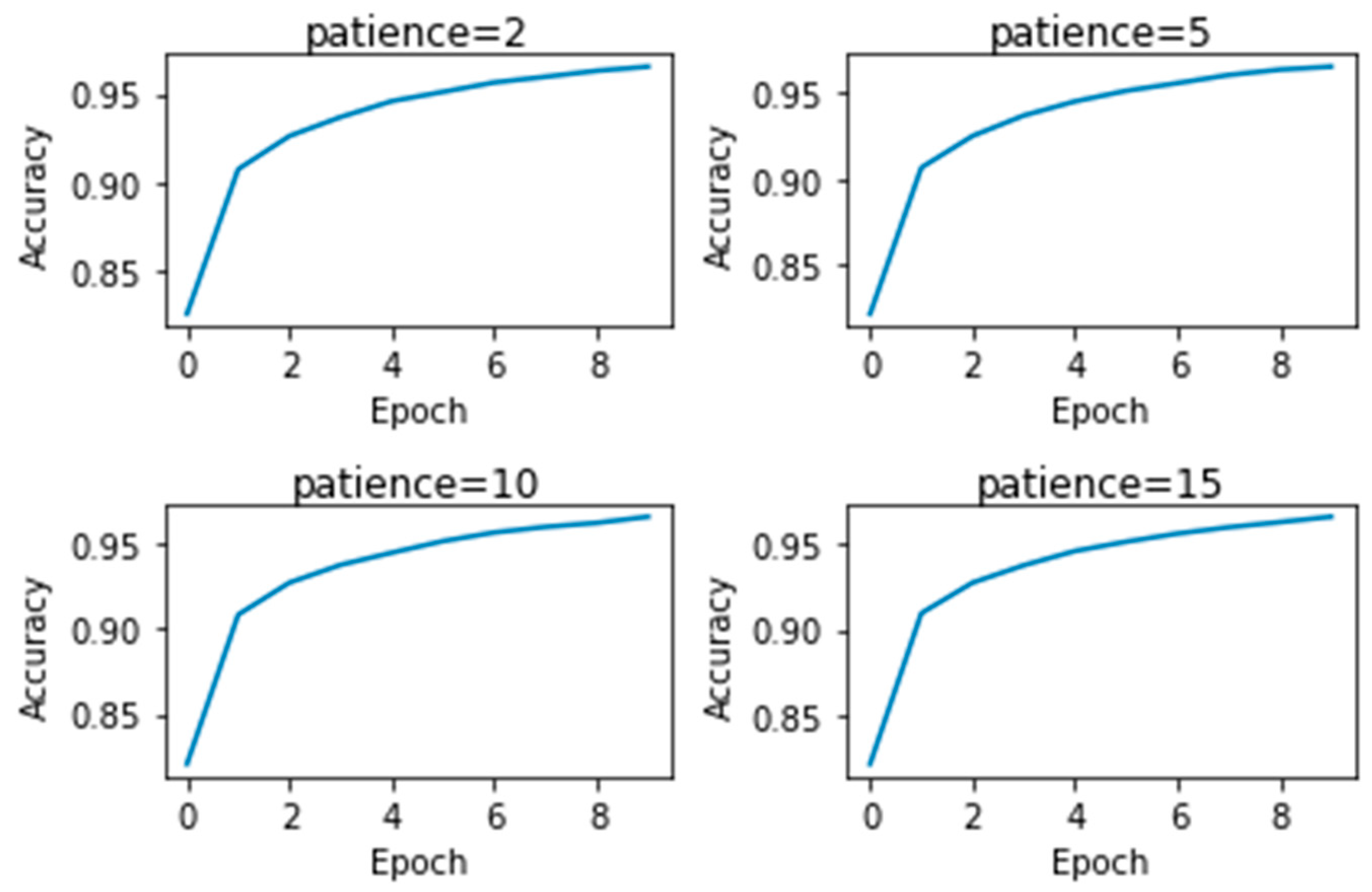
1 × 10−4	189.3757	14.288	0.1135

. We concluded that choosing a decay rate with 0.001 will yield the highest accuracy with the minimum test loss. The effect of changing patience was observed on CNN. The results are shown in Figure 3. We found that patience does not contribute much and tuning it would be of no significant value. In the end, different optimizers were used to check which works better for CNN. The results are shown in

Table 11. Effect of adaptive learning rate on CNN.

Optimizer	Execution Time (s)	Test Loss	Test Accuracy
sgd	197.060	14.5739	0.0958
adagrad	206.4216	0.0373	0.9884
rmsprop	210.9303	0.0940	0.9753
adam	227.1574	11.1512	0.3081

. From this chart, we conclude that accuracy is higher for the “adagrad” optimizer with the test loss being the least of all the values.

Our check was done by performing the experiment with epoch = 10, optimizer = adagrad, learning rate = 0.01. The results are as follows:

• Test loss: 0.037307307005505934;
• Test accuracy: 0.9884;
• Execution time 206.42161179700088 s.

4.2. Testing on RNN

We followed the same routine and we tested RNN by changing the values of our hyperparameters.

Table 12. Effect of learning rate on RNN.

Learning Rate	Execution Time (s)	Test Loss	Test Accuracy
1.0	537.8466	9.68	0.20
0.1	518.4978	1.34	0.50
0.01	543.3441	0.49	0.38
0.001	543.5569	0.35	0.91
1 × 10−5	545.0050	2.34	0.150
1 × 10−6	547.1852	2.471	0.089
1 × 10−7	548.0541	2.4478	0.0995

,

Table 13. Effect of momentum on RNN.

Momentum	Execution Time (s)	Test Loss	Test Accuracy
0.0	540.4106	1.3236	0.5065
0.5	550.4989	1.3187	0.5106
0.9	547.5802	1.4143	0.4721
0.99	546.3948	1.8778	0.344

,

Table 14. Effect of learning rate decay on RNN.

Decay Rate	Execution Time (s)	Test Loss	Test Accuracy
1 × 10−1	553.0807	2.1518	0.2003
1 × 10−2	547.6283	1.6197	0.4363
1 × 10−3	550.5157	1.3418	0.4953
1 × 10−4	554.0735	1.3091	0.5045

and

Table 15. Effect of adaptive learning rate on RNN.

Optimizer	Execution Time (s)	Test Loss	Test Accuracy
sgd	556.2208	1.3299	0.5006
adagrad	511.8971	1.2798	0.5153
rmsprop	554.7731	1.2300	0.5219
adam	507.3368	1.2263	0.5268

show the effect of changing learning rate, momentum, decay rate and optimizer, respectively, on RNN.

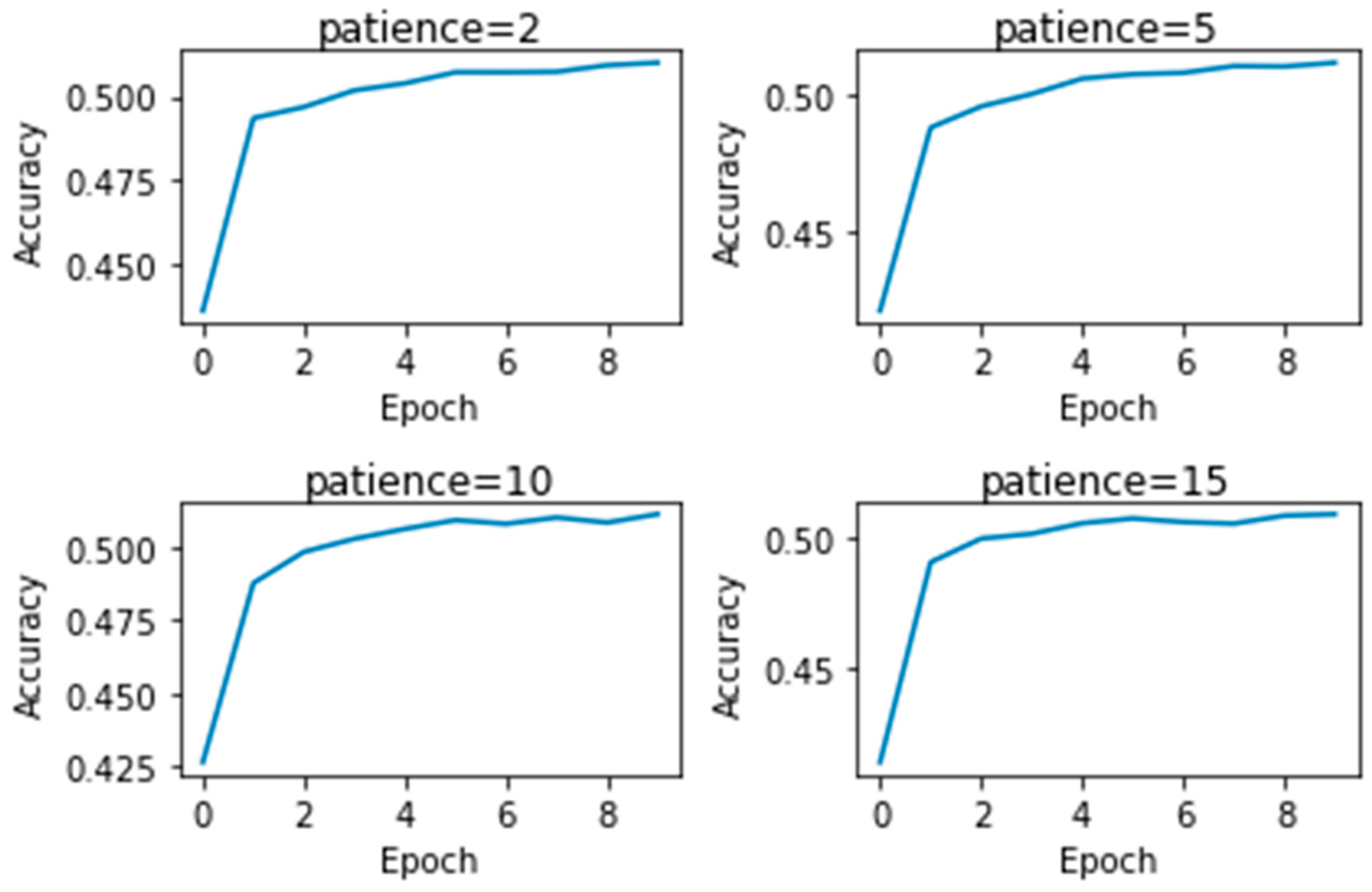
We see that even though momentum is up, the execution time is still above 540 s, which in turn converts to 9.5 min and above. The decay rate does affect accuracy, but in most cases, it does not significantly affect the execution time. However, we can see that there is no change in execution time with a change in learning rate; and the same is true for all the other hyperparameters, including patience, as shown in Figure 4. Moreover, there is no significant change in test accuracy by changing the hyperparameters. Consequently, we conclude that in the case of RNN, it is useless to tune the hyperparameters.

4.3. Testing on Multilayer Perceptron

We tested the multilayer perceptron by changing the values of our hyperparameters.

Table 16. Effect of learning rate on multilayer perceptron.

Learning Rate	Execution Time (s)	Test Loss	Test Accuracy
1.0	111.8561	0.35	0.93
0.1	114.1725	0.04	0.98
0.01	113.7956	0.10	0.97
0.001	113.6433	1.2	0.95
0.0001	110.7100	1.2	0.81
1 × 10−5	114.1752	2.20	0.26
1 × 10−6	114.1752	2.315	0.114
1 × 10−7	111.8580	2.320	0.069

,

Table 17. Effect of momentum on multilayer perceptron.

Momentum	Execution Time (s)	Test Loss	Test Accuracy
0.0	113.1584	0.0993	0.9693
0.5	113.5636	0.0715	0.9775
0.9	113.2237	0.0608	0.9833
0.99	110.3216	0.3334	0.9357

,

Table 18. Effect of learning rate decay on multilayer perceptron.

Decay Rate	Execution Time (s)	Test Loss	Test Accuracy
1 × 10−1	116.0973	1.7942	0.7002
1 × 10−2	118.7561	0.5041	0.8741
1 × 10−3	117.2670	0.2450	0.9299
1 × 10−4	116.5646	0.1357	0.9596

and

Table 19. Effect of adaptive learning rate on multilayer perceptron.

Optimizer	Execution Time (s)	Test Loss	Test Accuracy
sgd	115.6153	0.0983	0.97
adagrad	129.2784	0.0547	0.983
rmsprop	134.0489	0.1527	0.9793
adam	140.3749	0.0876	0.9788

show the effect of changing learning rate, momentum, decay rate and optimizer, respectively, on the multilayer perceptron model.

From the results, we can see that the best optimum learning rate is 0.1, giving the least loss and maximum accuracy. The best test accuracy was achieved with a moment value of 0.9. A decay rate of 0.0001 yields maximum test accuracy. The Patience value shows hardly any effect in boosting the test accuracy as shown in Figure 5. “Adagrad” outperforms all other optimizers in every criterion.

4.4. Testing on Siamese Neural Network (SNN)

We tested SNN by changing the value of our hyperparameters.

Table 20. Effect of learning rate on SNN.

Learning Rate	Execution Time (s)	Test Loss	Test Accuracy
1.0	133.8607	0.02	0.96
0.01	134.2296	0.075	0.91
0.001	135.2440	0.150	0.80
0.0001	136.8519	0.1	0.54
1 × 10−5	136.5850	0.1	0.57
1 × 10−6	134.1337	0.5	0.50
1 × 10−7	136.4893	0.7	0.50

,

Table 21. Effect of momentum on SNN.

Momentum	Execution Time (s)	Test Loss	Test Accuracy
0.0	137.4330	0.075	0.91
0.5	138.4175	0.06	0.93
0.9	140.5404	0.04	0.96
0.99	141.6775	0.04	0.95

,

Table 22. Effect of learning rate decay on SNN.

Decay Rate	Execution Time (s)	Test Loss	Test Accuracy
1 × 10−1	141.6452	17.5	0.56
1 × 10−2	141.5815	0.20	0.67
1 × 10−3	141.1553	0.12	0.83
1 × 10−4	141.6149	0.08	0.90

and

Table 23. Effect of adaptive learning rate on SNN.

Optimizer	Execution Time (s)	Test Loss	Test Accuracy
sgd	144.0273	0.08	0.90
adagrad	149.5838	0.08	0.97
rmsprop	151.4795	0.08	0.97
adam	159.8236	0.01	0.97

show the effects of changing learning rate, momentum, decay rate and optimizer, respectively, on the SNN model. From the results, we can see that a learning rate of 1.0 yields the maximum result; hence using it will be beneficial. A momentum of 0.9 or 0.99 yields maximum accuracy, hence it should be used. Moreover, decay with 0.0001 yields maximum accuracy, and the “adagrad” optimizer outperforms all optimizers, yielding high accuracy and converging in less execution time.

4.5. Testing on Knowledge Transfer Model

In the case of the knowledge transfer model, we have a base model and a transfer model, as shown in Table 7.

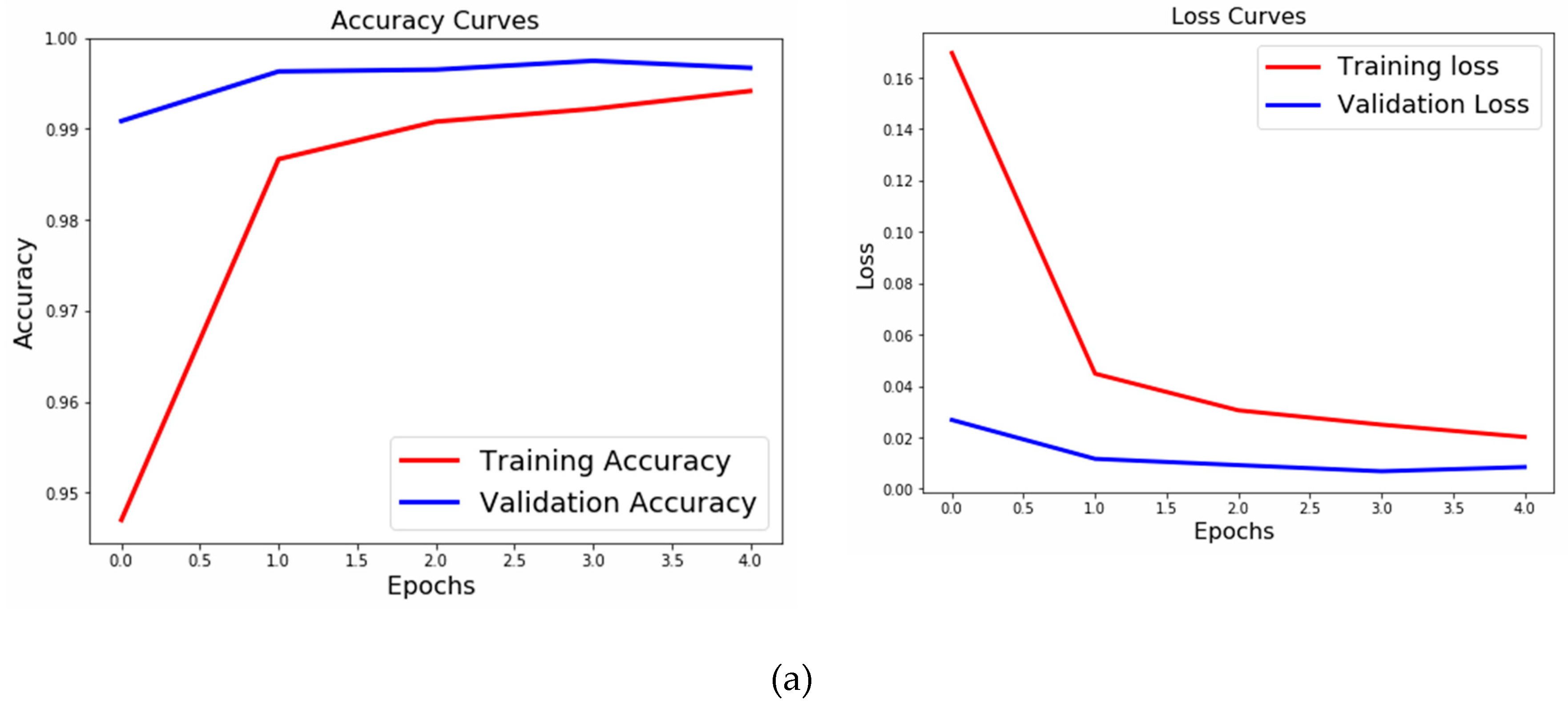
For the base model, we saw the following results:

• Training and execution time: 18.433 s;
• Test accuracy: 0.996.

Figure 6a shows the accuracy and a loss curve for the basic NN model of the knowledge-transfer model.

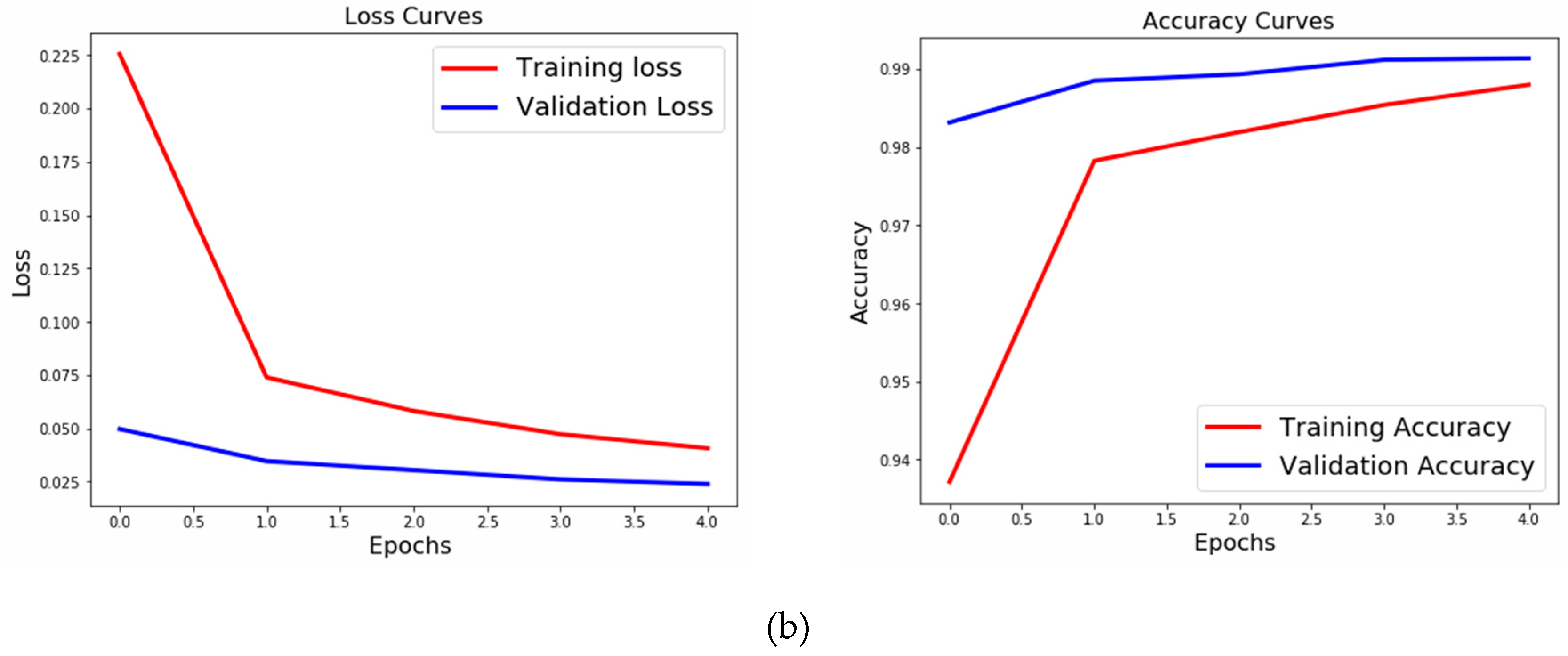
In the case of the transferred model, we saw the following results:

• Training and execution time: 11.73 s;
• Test accuracy: 0.991.

Figure 6b shows the accuracy and a loss curve for the transferred NN model of the knowledge-transfer model.

We can clearly see that the knowledge-transfer model outperforms all the models and takes significantly less time. We did not tune the patience, taking it to be 0. The learning rate was 0.01, with no decay rate.

We can see from

Table 24. Comparison of neural networks.

Decay Rate	Execution Time (s)	Test Loss	Test Accuracy
CNN	257.5474	0.314	1
RNN	537.8466	1.2129	0.5368
MLP	114.1725	0.04	0.98
Siamese Network	18.5591	0.0084	0.9961
Knowledge transfer	11.7357	0.0239	0.9931

that CNN outperforms all models, but the execution time is very high. The knowledge transfer model has the best model time with significantly less time and higher accuracy. The results of NNs are in Table 24 and were taken by choosing the best parameter values.

4.6. Parameters Influence and Discussion

The hyperparameters show a different impact on the convergence of the final trained model. Despite the selection of optimal hyperparameters, the model trained from the ground truth will not match the ground truth data precisely. The reason is that the dataset is just a proxy for the data distribution. With larger training samples, the trained model parameters will be close enough to the parameters used to generate the data. In general, if the batch size and the learning rate are correctly tuned, the model will quickly converge. In addition, an optimal and proper seeding of the model will help achieve optimization, thus enabling the model to converge to the best minimum out of several minima.

The learning rate plays a significant role in the convergence of the model towards the optimum. It is seen to counterbalance the cost function influence. If the learning rate chosen is comparatively large, the algorithm does not typically converge. If the selected learning rate is very low, the algorithm will need considerable time to achieve the desired accuracy. It can be seen from execution time in Table 8, Table 12, Table 16 and Table 20 that lower learning rate takes more execution time. If the learning rate is optimally selected and learning rate updates are in optimal settings, then the model should converge to a good set of parameters. From the influences of the learning rate vs. cost function of an algorithm’s convergence, we observed that the cost function influences a good learning rate. If the cost function is steep/highly curved, the larger the learning step size, the more the algorithm will not correctly and optimally converge. Therefore, taking small learning steps diminishes the overshoot problem; however, it also drastically slows the learning process and algorithm convergence.

Generally, in the machine learning community, a comparatively large learning rate is usually selected (between 0.1 and 1) and decayed while training on the data [30]. As such, we observed that the right decay selection is of immense importance. Decay selection involves two questions: how much decay and how often? Both of these are non-trivial. As such, we note that aggressively decaying settings extremely slow down the convergence of the model towards the optimum. On the other hand, very minute-paced decaying settings result in chaotic updates to the model, and very small improvements are observed. We conclude from the experiments that optimal decay schedules are of immense importance. Adaptive approaches such as RMSprop, Adam and Momentum help adjust the learning rate during convergence and optimization.

All the parameters chosen for tuning are related to the learning rate of the model. First, there is an inverse relationship between the learning rate and momentum. A high value of momentum can be compensated with a low learning rate in order to achieve high accuracy and vice versa. However, there is still a threshold that needs to be maintained in order to achieve high accuracy, i.e., very smaller values of momentum cannot be compensated with increasing high value of learning rate. It can be seen from Table 8 and Table 9 that maximum accuracy was achieved while keeping learning rate low, but not too low and momentum value high, but not too high. The similar is true for Table 12 and Table 13 although in case of RNN model optimal momentum value is smaller than CNN, which is acceptable as each model has its own optimal values of parameters. In Table 16 and Table 17, the learning rate has gone up 10 times, but the momentum value remains 0.9. In case of knowledge-transfer model, Table 20 and Table 21, the learning rate is high, but momentum value is still 0.9 for highest accuracy, this can be explained in a sense that it is not appropriate to say which learning rate is appropriate for the model, i.e., not too high or not too low. Second, when comparing the learning rate with the decay rate, it is important to notice that a high decay rate can cause the model never to reach an optimal point if the learning rate value is small, while the low decay rate can cause the model to pass the optimal point while keeping the learning rate high. Therefore, it can be concluded that a high decay rate can be compensated with a high learning rate while a low decay rate can be compensated with a low learning rate. This can be proved using Table 8 and Table 10, Table 12 and Table 14, Table 16 and Table 18 where low learning rate and low decay rate gives highest accuracy. For Table 20 and Table 22 this is also true if we consider learning rate as low for knowledge-transfer model. Hence, when looking it altogether low learning rate, high momentum value and low learning decay rate gives higher accuracy. However, while decreasing the learning rate at plateau makes the model more accurate, it would also decrease the learning rate and affect the other parameters linked to it, as explained above. This can help make an overview of the whole structure about the dependency of hyperparameters on each other taking the learning rate as the base.

In the end, the adaptive learning rate helps in compensating the effect of poorly configured learning rate. Choosing an optimizer does not affect the other parameters that much and it is not dependent on their values. Although choosing an appropriate optimizer is also important according to different neural networks models. When speaking in terms of execution time Adam optimizer has a highest execution time followed by RMSProp. This is true for all the cases in Table 11, Table 19 and Table 23, except for Table 15 where in case of RNN model SGD has highest execution time. When dealing with execution time it is also important to mention effect of batch size on it. High batch size causes a low number of batches for training which in return causes less training time. There is not much difference in final accuracy, but higher batch size takes less iteration to reach it and lower batch size takes more time to reach it [22].

5. Conclusions and Future Work

There are many neural network models; each one is unique in its own way. It has been shown that when comparing different models for a specific set and the values of hyperparameters, the “knowledge-transfer model” outperforms all other models. It is true that CNN also gives great results, but at the cost of high execution time. This research is useful in the sense that while building a specific classification model, one can select the values of hyperparameters that perform better according to the proof given.

Everything is incomplete and there is always room for improvement. In our opinion, one can apply an algorithm for hyperparameter tuning to test the performance of the model. This may lead to better hyperparameter value selection and hence provides better classification results.

References

- Fukushima, K.; Miyake, S.; Ito, T. Neocognitron: A neural network model for a mechanism of visual pattern recognition. IEEE Trans. Syst. Man Cybern. 1983, 826–834. [Google Scholar] [CrossRef]
- LeCun, Y.; Boser, B.; Denker, J.S.; Henderson, D.; Howard, R.E.; Hubbard, W.; Jackel, L.D. Backpropagation applied to handwritten zip code recognition. Neural Comput. 1989, 1, 541–551. [Google Scholar] [CrossRef]
- Bakhshi, A.; Chalup, S.; Noman, N. Fast Evolution of CNN Architecture for Image Classification. In Deep Neural Evolution; Springer: Singapore, 2020; pp. 209–229. [Google Scholar]
- Pearlmutter, A. Learning state space trajectories in recurrent neuralnetworks. Neural Comput. 1989, 1, 263–269. [Google Scholar] [CrossRef]
- Sherstinsky, A. Fundamentals of recurrent neural network (RNN) and long short-term memory (LSTM) network. Phys. D Nonlinear Phenom. 2020, 404, 132306. [Google Scholar] [CrossRef]
- Li, D.; Wang, H.; Li, Z. Accurate and Fast Wavelength Demodulation for Fbg Reflected Spectrum Using Multilayer Perceptron (Mlp) Neural Network. In Proceedings of the 2020 12th International Conference on Measuring Technology and Mechatronics Automation (ICMTMA), Phuket, Thailand, 28–29 February 2020; Institute of Electrical and Electronics Engineers (IEEE): Piscataway, NJ, USA, 2020; pp. 265–268. [Google Scholar]
- Albahli, S. A deep ensemble learning method for effort-aware just-in-time defect prediction. Future Internet 2019, 11, 246. [Google Scholar] [CrossRef]
- Chopra, S.; Hadsell, R.; LeCun, Y. Learning a Similarity Metric Discriminatively, with Application to Face Verification. In Proceedings of the 2005 IEEE Computer Society Conference on Computer Vision and Pattern Recognition (CVPR 05), San Diego, CA, USA, 20–26 June 2005; Institute of Electrical and Electronics Engineers (IEEE): Piscataway, NJ, USA, 2005; pp. 539–546. [Google Scholar]
- Vinayakumar, R.; Soman, K.P. Siamese neural network architecture for homoglyph attacks detection. ICT Express 2020, 6, 16–19. [Google Scholar] [CrossRef]
- Bacanin, N.; Bezdan, T.; Tuba, E.; Strumberger, I.; Tuba, M. Optimizing convolutional neural network hyperparameters by enhanced swarm intelligence metaheuristics. Algorithms 2020, 13, 67. [Google Scholar] [CrossRef]
- LeCun, Y.; Cortes, C.; Burges, C.J. MNIST Handwritten Digit Database. 2010. Available online: www.research.att.com/~yann/ocr/mnist (accessed on 28 March 2020).
- Kussul, E.; Baidyk, T. Improved method of handwritten digit recognition tested on MNIST database. Image Vis. Comput. 2004, 22, 971–981. [Google Scholar] [CrossRef]
- Koch, G.; Zemel, R.; Ruslan, S. Siamese neural networks for one-shot image recognition. In Proceedings of the ICML Deep Learning Workshop, Bonn, Germany, 7–11 August 2005; Volume 2. [Google Scholar]
- Li, S.; Li, W.; Cook, C.; Zhu, C.; Gao, Y. Independently Recurrent Neural Network (IndRNN): Building A Longer and Deeper RNN. In Proceedings of the 2018 IEEE/CVF Conference on Computer Vision and Pattern Recognition, Salt Lake City, UT, USA, 18–22 June 2018; Institute of Electrical and Electronics Engineers (IEEE): Piscataway, NJ, USA, 2018; pp. 5457–5466. [Google Scholar]
- Liu, C. Probabilistic Siamese Networks for Learning Representations. Ph.D. Thesis, University of Toronto, Toronto, ON, Canada, 2013. [Google Scholar]
- Chen, L.; Wang, S.; Fan, W.; Sun, J.; Naoi, S. Beyond human recognition: A CNN-based framework for handwritten character recognition. In Proceedings of the 2015 3rd IAPR Asian Conference on Pattern Recognition (ACPR), Kuala Lumpur, Malaysia, 3–6 November 2015; Institute of Electrical and Electronics Engineers (IEEE): Piscataway, NJ, USA, 2015; pp. 695–699. [Google Scholar]
- Niu, X.X.; Suen, C.Y. A novel hybrid CNN–SVM classifier for recognizing handwritten digits. Pattern Recognit. 2012, 45, 1318–1325. [Google Scholar] [CrossRef]
- Agarap, A.F. An architecture combining convolutional neural network (CNN) and support vector machine (SVM) for image classification. arXiv 2017, arXiv:1712.03541. [Google Scholar]
- Zhang, H.; Berg, A.; Maire, M.; Malik, J. SVM-KNN: Discriminative Nearest Neighbor Classification for Visual Category Recognition. In Proceedings of the 2006 IEEE Computer Society Conference on Computer Vision and Pattern Recognition—Volume 1 (CVPR’06), Washington, DC, USA, 27 June–2 July 2006; Institute of Electrical and Electronics Engineers (IEEE): Piscataway, NJ, USA, 2006; Volume 2, pp. 2126–2136. [Google Scholar]
- Vlontzos, A. The RNN-ELM classifier. In Proceedings of the 2017 International Joint Conference on Neural Networks (IJCNN), Anchorage, Alaska, 14–19 May 2017; Institute of Electrical and Electronics Engineers (IEEE): Piscataway, NJ, USA, 2017; pp. 2702–2707. [Google Scholar]
- Loshchilov, I.; Hutter, F. CMA-ES for Hyperparameter optimization of deep neural networks. arXiv 2016, arXiv:1604.07269. [Google Scholar]
- Smith, L.N. A disciplined approach to neural network hyper-parameters: Part 1—Learning rate, batch size, momentum, and weight decay. arXiv 2018, arXiv:1803.09820. [Google Scholar]
- Domhan, T.; Springenberg, J.T.; Hutter, F. Speeding up automatic hyperparameter optimization of deep neural networks by extrapolation of learning curves. In Proceedings of the Twenty-Fourth International Joint Conference on Artificial Intelligence, Buenos Aires, Argentina, 25–31 July 2015; pp. 3460–3468. [Google Scholar]
- Bardenet, R.; Brendel, M.; Kegl, B.; Sebag, M. Collaborative hyperparameter tuning. In Proceedings of the International Conference on Machine Learning, Atlanta, GA, USA, 16–21 June 2013; pp. 199–207. [Google Scholar]
- Koutsoukas, A.; Monaghan, K.J.; Li, X.; Huan, J. Deep-learning: Investigating deep neural networks hyper-parameters and comparison of performance to shallow methods for modeling bioactivity data. J. Chemin. 2017, 9, 42. [Google Scholar] [CrossRef] [PubMed]
- Rastegari, M.; Ordonez, V.; Redmon, J.; Farhadi, A. XNOR-Net: Imagenet classification using binary convolutional neural networks. In Proceedings of the European Conference on Computer Vision, Amsterdam, The Netherlands, 11–14 October 2016; Springer: Amsterdam, The Netherlands, 2016. [Google Scholar]
- Dutta, K.; Krishnan, P.; Mathew, M.; Jawahar, C. Improving CNN-RNN Hybrid Networks for Handwriting Recognition. In Proceedings of the 2018 16th International Conference on Frontiers in Handwriting Recognition (ICFHR), Niagara Falls, NY, USA, 5–8 August 2018; Institute of Electrical and Electronics Engineers (IEEE): Piscataway, NJ, USA, 2018; pp. 80–85. [Google Scholar]
- Li, L.; Jamieson, K.; Rostamizadeh, A.; Gonina, E.; Hardt, M.; Recht, B.; Talwalkar, A. Massively parallel hyperparameter tuning. arXiv 2018, arXiv:1810.05934. [Google Scholar]
- Shang, X.; Kaufmann, E.; Valko, M. A simple dynamic bandit algorithm for hyper-parameter tuning. In Proceedings of the 6th ICML Workshop on Automated Machine Learning, Long Beach, CA, USA, 14–15 June 2019. [Google Scholar]
- Sanodiya, R.K.; Mathew, J.; Saha, S.; Thalakottur, M.D. A New transfer learning algorithm in semi-supervised setting. IEEE Access 2019, 7, 42956–42967. [Google Scholar] [CrossRef]
Figure 1.
An un-rolled recurrent neural network.
Figure 2.
Handwritten digit recognition in MNIST (Modified National Institute of Standards and Technology) database.
Figure 3.
Effect of patience value on CNN.
Figure 4.
Effect of patience value on RNN.
Figure 5.
Effect of patience value on MLP.
Figure 6.
Performance curves for knowledge-transfer model. (a) Performance curves for basic knowledge-transfer model for accuracy (left) and loss (right); (b) performance curves for transferred knowledge-transfer model for accuracy (left) and loss (right).