Heat Transfer Performance in Energy Piles in Urban Areas: Case Studies for Lambeth College and Shell Centre UK

Abstract

A ground source heat pump system is a highly efficient renewable heating, cooling, and ventilation system that utilizes the ground as a heat source or sink via ground heat exchangers. Energy pile is an energy geotechnical structure that couples a ground heat exchanger with a geotechnical structure, leading to low capital cost. The design of energy piles can be challengeable due to their complicated geometries and the requirement of mechanical load. This study focuses on the heat transfer across the concrete–soil interface of energy piles in urban areas. Case studies from two projects, the Lambeth College and Shell Centre projects, are presented and discussed. The back analysis of two energy pile cases illustrated that the heat transfer coefficient at the pile–soil interface can differ between the cooling mode and the heating mode. It can be concluded that the difference in the heat transfer coefficient is influenced by a number of factors such as soil properties, concrete (grout) properties, and the installation method.

1. Introduction

The ground source heat pump (GSHP) has been widely approved as an effective and renewable technology towards energy saving and CO₂ emission reduction [1,2,3]. However, the implementations of GSHPs are not processed well due to the high initial capitalization [4,5,6,7]. Although GSHP may cut the energy cost by 30%–70%, the payback period in the UK is generally over 10 years [8]. In the UK and Northern Europe, a great budget has been used to encourage the application of GSHPs [9]. To install the GSHP loops into geotechnical infrastructure can avoid the borehole drilling cost so it leads to great saving for GSHP application. Geotechnical Structures with GSHP loops, so called energy geotechnical structures (EGS), are thriving in the UK, while projects have been built and operated of installing GSHP loops into piles, diaphragm walls, and so called energy piles and thermal walls [8].

The design of such EGSs cannot follow the classic method for borehole heat exchangers (BHEs) due to their complicated geometries and the requirement of mechanical load. As well, the energy geotechnical structures are always built near underground spaces such as tunnels, basements, or station boxes which send off heat flux and influence the heating capacity of GSHPs [10]. The complex thermal behavior of energy piles and thermal walls requires careful design considering many details which are ignored in the BHE designs. Evaluation of the heat transfer efficiency in an energy pile is of significance in its design. In BHE this can be done by a Thermal Response Test (TRT) [11], which generates an “overall” thermal conductivity of the ground. However, in energy piles which have a bigger diameter than BHEs, the heat transfer process is more complicated. If hot water is injected, heat flux transfers across the pipe wall to the concrete pile body, then to the ground. Therefore, several factors contribute to the thermal conductivity value of the whole energy pile such as the pipe wall, the concrete property, the film resistance at the concrete–soil interface, and the ground properties. This study focuses on the heat transfer across the concrete–soil interface of energy piles in urban areas. The data from the Lambeth College and Shell Centre projects are reviewed. Issues related to the heat transfer coefficient values in heating/cooling operation modes are presented.

2. Energy Piles

Initial studies into EGSs were recorded for several cases in Austria, including both piles and walls [10]. In subsequent decades energy piles have been installed in many countries, including the UK [12,13] and China [11]. As an example, Brandl (2006) reported that the total number of energy piles installed in Austria increased by almost an order of magnitude in the period from 1990 to 2004 [10]. In the UK, the first energy piles were installed at Keble College in Oxford in 2001 [14]. Since then, installation of energy foundations has increased rapidly. Just 150 energy piles were installed per year in the UK in 2004; by 2008 this had risen to nearly 1600 energy piles per year [15]. After 2010 the rate of increase has reduced in line with the economic situation [12], but there still remains significant interest in this relatively new technology. There are landmark GSHP coupled foundation schemes such as “One New Change” Project [16] with both energy piles and open loop GSHP wells. Moreover, several energy-pile projects have been built, operated, and published [12,14,17].

Until recently, energy piles were mainly built as driven precast concrete piles with integrated heat exchange tubes. Since 2000, the technology has been extended to large-diameter bored piles, where the size of the pile allows for placing multiple U-shaped loops of pipes used to circulate the carrier fluid. In bored energy piles the pipes are typically made of high-density polyethylene, 20–25 mm in diameter and about 2 mm thick and are fixed to the reinforcement cage. Heat carrier fluid used in the primary circuit can be water, saline solutions or water-glycol mixtures, with the latter having been proven to be the most suitable option in most cases due to their good antifreeze properties and low environmental impact as a result of their low toxicity and high biodegradability. The fluid flow rates, and pipe diameters are selected to achieve turbulent flow conditions that enhance heat transfer and obtain the required amount of heat transfer [18].

Determination of diameter, material, flow rates and pipe size, etc. requires careful design work. The design of energy piles is more complicated than for BHE since energy piles play double roles. They not only work as piles holding the mechanical load of the building, but also as underground heat exchangers which extract heat from or inject heat into the ground. Although a standard framework for energy pile design has been produced by the Ground Source Heat Pump Association (GSHPA) in the UK, further work is needed to help engineers make design decisions about thermal behaviors, and especially for energy piles. The next section will illustrate the background and methodology to analyze the data from the Lambeth College and Shell Centre projects, which could assist in the wider application of energy piles.

3. Background and Methodology

In general, the TRT (Thermal Response Test) method is employed to estimate the thermal properties of energy piles [11]. However, the accuracy of TRT for energy piles can be lower than that for BHEs because of the complicated components in energy piles. Loveridge et al. [13] developed a numerical approach for calculating the thermal resistance of an energy pile. The parameter discussed in Loveridge’s model contains the pipe wall thermal resistance, the concrete properties and the position of the heat exchanger loops. However, there are still components of the thermal resistance that were not considered, such as the in-pipe layer resistance and the thermal resistance at the surface of the pile. If all these components are fully simulated, the TRT data could be used to determine the ground thermal properties more accurately by numerical back analysis.

This study aims to illustrate the heat transfer at the concrete–soil surface of EGSs. In the simplest case, heat transfer across an interface follows Figure 1.

$$Q=h\left(T_2-T_1\right)$$

(1)

where Q is the heat flux (W/m²), h is the heat transfer coefficient (Wm⁻²K⁻¹), and $T_2$ and $T_1$ are the temperature values at the two sides of the interface.

One of the concerns in energy pile design relates to the expansion and contraction of the pile caused by temperature changes. As shown in Figure 1, it can be assumed that the tightness of contact between the soil and the concrete decreases when the pile contracts. As a result, the heat transfer across this interface could become inefficient. Conversely, in the pile heating period, the concrete pile body is hotter than the soil, and thus the pile expands and causes the heat transfer coefficient to increase.

Normal operation of the energy piles includes both heating and cooling modes. Accordingly, the heat transfer coefficient from the pile body to the surrounding soil may vary, and thus the heat extraction/injection rate of the energy pile may not be constant. Ideally the design operation plan should take this into account. Olgun et al. [19] has noticed this difference by studying a radial expansion of an energy pile in US, and potential effects on contact pressures were discussed. However, to the best of author’s knowledge there has been no research about the contact thermal resistance. Ignorance of this issue could lead to differences between the design and the real operation in the long run.

The thermo-mechanical issue of an energy pile was discussed in work by Amis et al. [20] in their project in Lambeth College. Lambeth College is situated in South London and uses all 143 of its bored pile foundations as energy piles. Prior to its construction a trial was carried out by Cementation Skanska, Geothermal International Ltd., and Cambridge University, which involved the installation of a test pile that was subjected to extreme heating and cooling cycles. The intention of the trial was to improve the understanding of what impacts heating and cooling cycles have on the structural and/or geotechnical performance of a pile, and to analyze the thermodynamic response of the system [17]. The mechanical behavior of an energy pile was recorded with a heating-cooling trial. In the pile, the strain was detected by means of both VWSG (Vibrating Wire Strain Gauges) and OFS (Optical Fiber Sensors) sensors. The details of the thermal-mechanical loading test of Lambeth College pile can be found from Amis’ work [20]. The test shows clearly that in the pile cooling mode, the concrete pile body contracts at both axial and radial directions for the strain curves are under zero. Meanwhile, in the pile heating period the pile expands, and the strain is positive.

Another TRT test was conducted in 2012 at the Shell Centre, London, to determine the overall thermal conductivity of an energy pile. The TRT operators faced similar problem in the data fitting from the hot/cold trial. In the end, different thermal conductivity values were eventually generated separately for the heating mode and cooling mode. The data from this test will be analyzed numerically in this study.

In this study, the Lambeth College case and the Shell Centre case are analyzed numerically in a 3D model via COMSOL Multiphysics, the details regarding of the methods are as below:

In industrial applications, it is common that the density of a process fluid varies. These variations can have a number of different sources but the most common is the presence of an inhomogeneous temperature field. The module used in this study includes the Non-Isothermal Flow predefined Multiphysics coupling to simulate systems where density varies with temperature. The model is based on the fully compressible formulation of the continuity equation and momentum equations:

$$\frac{\partial p}{\partial t}+\nabla ·(\rho \mathbf{u})=0$$

(2)

$$\rho \frac{\partial \mathbf{u}}{\partial \mathrm{t}}+\rho \mathbf{u}·\nabla \mathbf{u}=-\nabla p+\nabla ·(\mu (\nabla \mathbf{u}+{(\nabla \mathbf{u})}^{\tau }-\frac{2}{3}\mu (\nabla ·\mathbf{u})I)+F$$

(3)

where ρ is the density (kg/m³), u is the velocity vector (m/s), p is the pressure (Pa), μ is the dynamic viscosity (Pa·s), and F is the body force vector (N/m³).

The heat equation is:

$$\rho C_p(\frac{\partial \mathrm{T}}{\partial \mathrm{t}}+(\mathbf{u}·\nabla )\mathrm{T})=-(\nabla ·\mathbf{q})+\tau ·\mathrm{S}-\frac{\mathrm{T}}{\rho }\frac{\partial \rho }{\partial \mathrm{T}}\left(\frac{\partial p}{\partial \mathrm{t}}+(\mathbf{u}·\nabla )p\right)+Q$$

(4)

where in addition to the quantities above, C_p is the specific heat capacity at constant pressure (J/(kgK)), T is the absolute temperature (K), q is the heat flux by conduction (W/m²), τ is the viscous stress tensor (Pa), S is the strain-rate tensor (1/s), and Q contains heat sources other than viscous heating (W/m³).

The data were taken from research works concentrated on the heating-cooling circles [21]. The parameter “heat transfer coefficient at the soil-concrete interface” is examined. By conducting a series of parametric simulations, the heat transfer coefficient values in the heating or cooling modes are investigated.

4. The Lambeth College Case

4.1. Basic Information

Lambeth College is situated in South London and uses all 143 of its bored pile foundations as energy piles. Prior to its construction a trial was carried out by Cementation Skanska, Geothermal International Ltd., and Cambridge University, which involved the installation of a test pile that was subjected to extreme heating and cooling cycles. The intention of the trial was to improve the understanding of what impacts heating and cooling cycles have on the structural and/or geotechnical performance of a pile and to analyze the thermodynamic response of the system [17].

The TRT carried out on the Lambeth College test pile was analyzed. The TRT was selected from a part of the data monitored during the project. The object of the project was a load test with heating and cooling. The test pile was initially subjected to a period of loading alone between the dates of the 14th and 15th June 2007, before being subjected to a cooling mode cycle on 18th June, lasting for four weeks, in which the input fluid temperature in the ground loop was −6 °C. On 19th July the pile was then heated, using an input fluid temperature of 40 °C, until 31st July.

The test pile was fabricated with a nominal diameter of 610 mm through the made ground and terrace deposits, and 550 mm through the London clay. Its length was designed to be 23 m in order to resist the required working load of 1200 kN and to include a safety factor of 2.5. The ground loops and instrumentation required for the test were attached to the pile reinforcement cage, which consisted of six 32 mm diameter bars.

The details of the layout of the components used in the test can be found in [17]. In addition to the construction of the test pile, four anchor piles were installed 2 m away in order to simulate the load of the building. A heat sink pile was positioned 20 m away from the test pile so that heat could be transferred to and from it via an 8 kW heat pump which provided the heating and cooling outputs. In addition, a borehole containing instrumentation was constructed 0.5 m away from the test pile to record the nearby temperature profile. Two data loggers were also installed to record and analyze results from the instrumentation installed in each component.

Optical Fiber Sensors (OFS) were installed in the test energy pile and in the borehole in order to collect temperature and strain data. The details of how this instrumentation was embedded within the test pile and borehole can be found in [17]. Optical fibers enabled continuous distributed strain and temperature profiles to be measured, instead of the point measurements taken by more well-known equipment such as strain gauges. This technology is, therefore, ideal for monitoring the performance of piles. Thermistors (in the vibrating wire strain gauges) were also installed in the test energy pile to compare to the data measured by the OFS. VWSG thermistors that were located at the depth shown in

Table 1. Depth of VWSG groups in the borehole.

VWSG Group	VWSG1	VWSG2	VWSG3	VWSG4	VWSG5
Depth	1.5 m	4 m	6.5 m	10.5 m	16.5 m

, which shows how the temperature of the test pile changed over time at 9 m below ground level (bgl), and highlights the main activities carried out during the trial. The strain and mechanical results were analyzed by [17].

In this study, the temperature data of the project are used to discuss the change of heat transfer co-efficient across the pile-soil interface. The temperature was collected by both OFS and thermistors. There was a borehole 0.5 m away from the test pile. Thermistors and OFS were also installed into the borehole to monitor the ground temperature. These data are used to evaluate the heat transfer coefficient values in cooling and heating modes separately.

4.2. Methods

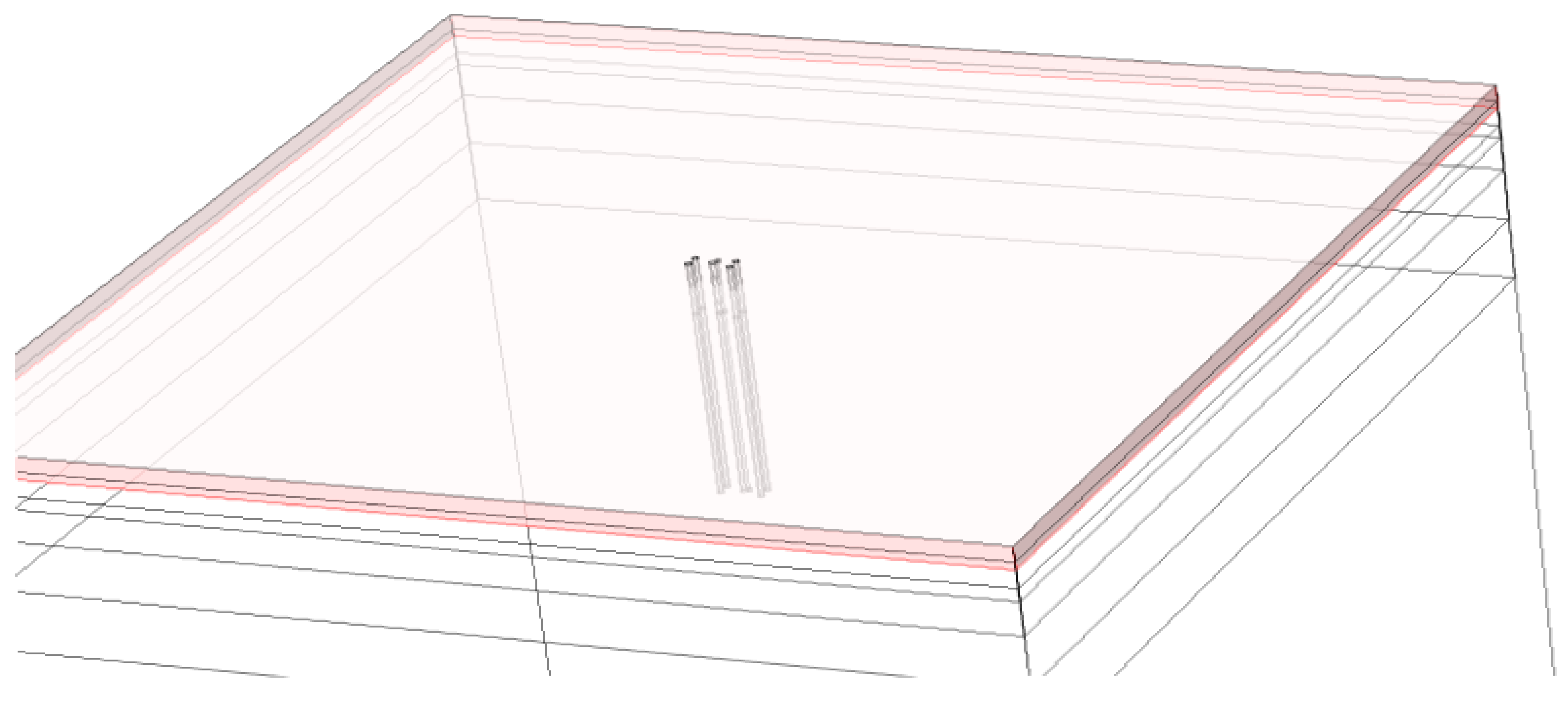
The methods of this case study are to simulate the thermal performance of the pile using an FE model. The model is shown in Figure 2. The energy pile was carefully simulated as a hollow cylinder while the anchor piles were solid concrete cylinders. The heat sink pile was not included in this model. The monitored temperature was applied at the inner surface of the test pile as its boundary condition. The borehole was simulated as a line 0.5 m away from the test pile. The layers in the soil were carefully simulated. The model included 1,227,964 elements (Figure 3).

The simulation was processed by back-analysis. The temperature profiles recorded by the OFS were input as boundary conditions at the positions where the OFS was installed. The calculated ground temperature profile in the borehole was plotted and compared to the recorded borehole temperature data. The aim of this back analysis was to approach the ideal situation in which the calculated ground temperature fits the record. The fluid flow here is simulated as a Modified Linear Model, which can ensure the model be solved as well as the accuracy of the heat transfer as a CFD Model [8].

It was assumed that the heat transfer coefficient value changes when the operation mode switches from the heating mode to the cooling mode. Therefore, in the simulation, this value was set as time dependent. During the heating mode or the cooling mode, different heat transfer coefficient values were applied, and the simulation was run with each value to find the best one.

5. The Shell Centre Case

5.1. Basic Information

The Shell Centre in London is one of the two “central offices” of the oil major Shell (the other is in The Hague). It is located on Belvedere Road in the London Borough of Lambeth. It is a prominent feature on the South Bank of the River Thames near County Hall, and now forms the backdrop to the London Eye.

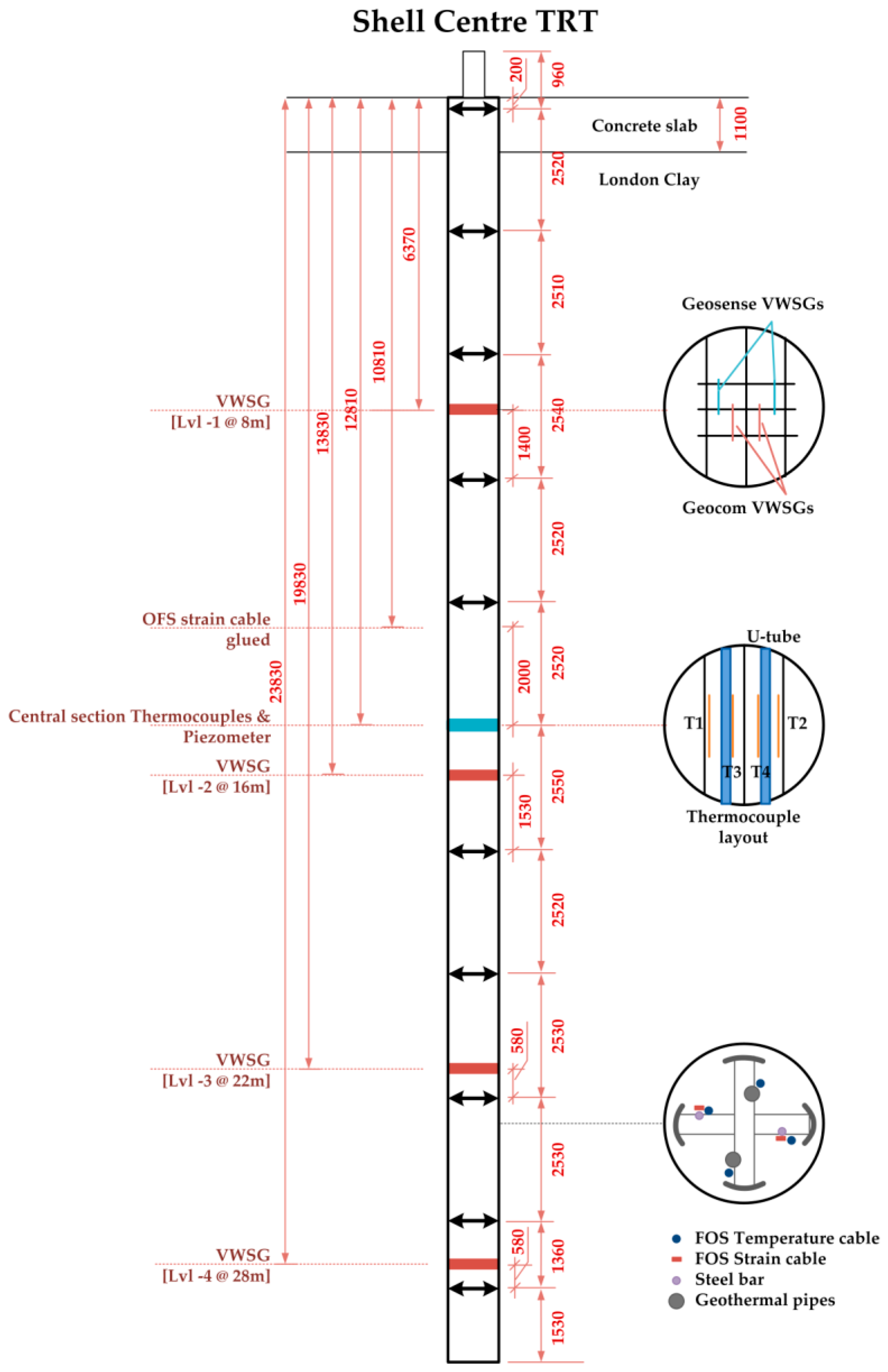
In 2012 a TRT was carried out in the Shell Centre to determine the ground thermal properties for the potential use of energy piles. As shown in Figure 4, a geotechnical borehole was initially drilled down to a depth of 26.8 m to investigate the ground conditions, water level, and to take samples for geotechnical testing. This borehole was then enlarged to 300 mm for the installation of a mini-energy pile. This energy pile was planned to be constructed from the existing ground level with roughly 10 m of casing penetrating through the 3 levels of car park down to the basement. A small reinforcement cage was designed to cater for the purpose of attaching all instrumentation. The central pipe was connected to a base plate and a series of specially designed spacers for mounting all instrumentations and the geothermal pipe.

Similar to the Lambeth College case, OFS and VWSGs were installed into the pile to detect changes in both strain and temperature. However, in this case the ground temperature some distance away from the borehole was not recorded.

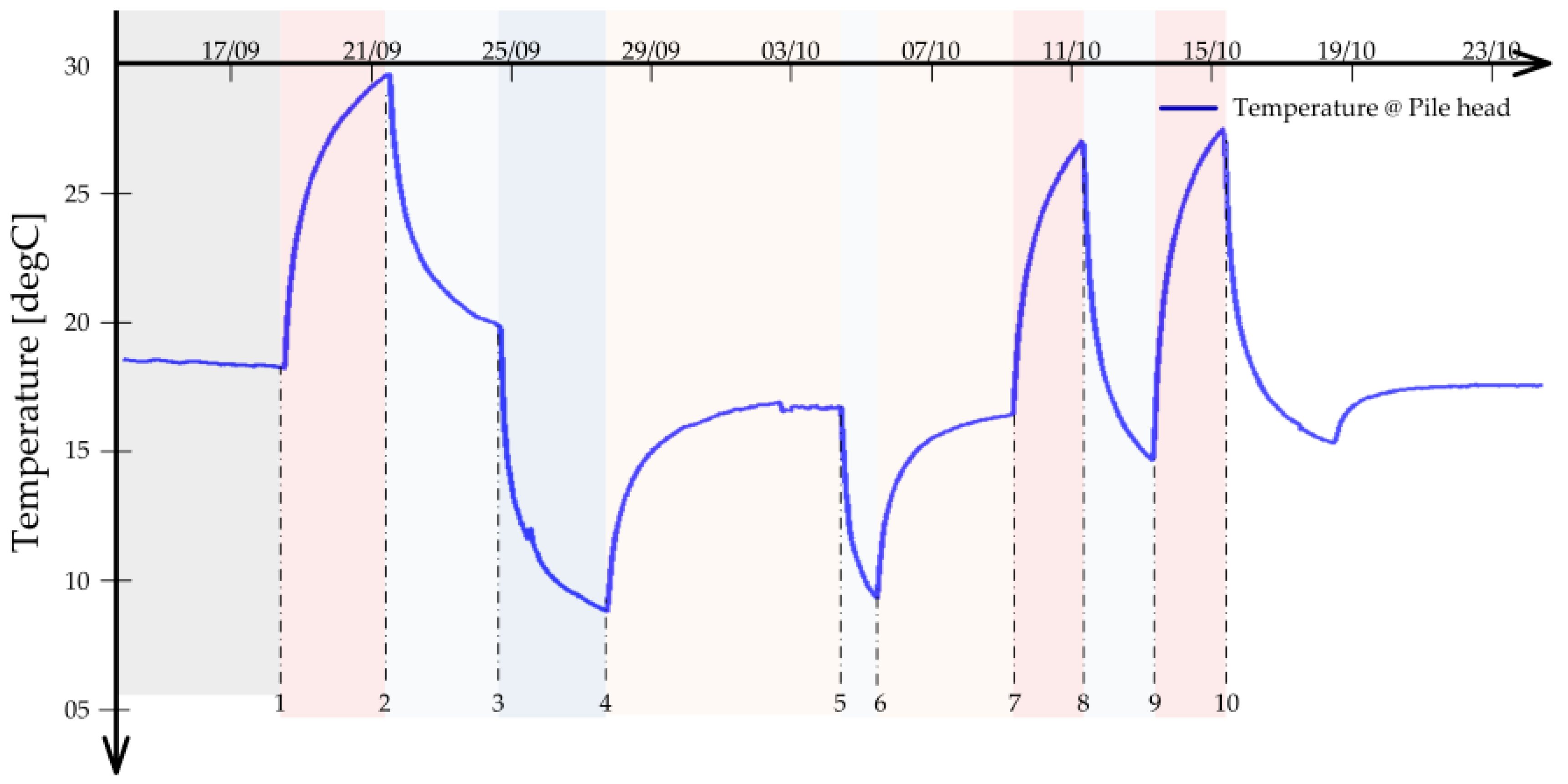
After the installation of the instrumented energy pile was completed, the VWSG data logger was set up and started recording measurements. Figure 5 summarizes the start date and measuring period of the instruments corresponding to the TRT with further details available in

Table 2. Parameters for Shell Centre model.

Geometry (Unit: m)	Pile geometry	Length			26
		Diameter			0.3
		Pipe position (pipe centre–borehole center)			0.05
	Soil box geometry	Length			25
		Height			50
		Width			25
	Pipe geometry	Diameter			0.040
		Wall thickness			0.004
Properties		Thermal Conductivity (W/m.K)	Density kg/m3	Heating Capacity J/kg.K	Viscosity m2/s × 10−6
	Soil	2.34	1800	1200	-
	Pile body (Concrete)	0.80	2300	880	-
	Heat carrying liquid	0.58	1050	3850	3.0
	Pipe wall (PVC)	0.16	1420	1000	-

.

5.2. TRT Results

The TRT results are shown in Figure 6 and Figure 7. In Figure 6, the field temperature data are recorded. The blue and red curves represent the inlet and outlet temperature profiles at the two ends of the loop. The green curve shows the average temperature which is calculated for the TRT. The yellow and purple curves at the bottom of the figure mean the flow rate and power injected into the energy pile. The average temperature curve (green curve) is plotted against the logarithm time value (Figure 6). Following the classic calculation, the thermal conductivity of the whole energy pile has two values in the heating mode and cooling mode circles. In the heating mode it is calculated as 2.34 Wm⁻¹K⁻¹, while in the cooling mode period it increases to 2.37 Wm⁻¹K⁻¹. The difference is small and can be ignored in the engineering project, but in this study, it is taken into account to investigate the heating/cooling mode effect to the energy pile.

The thermal conductivity value varied as the cooling/heating operations switched. This means the whole situation changed. The only condition that changed in this process was the temperature. Therefore, it can be assumed that the temperature change led to the thermal conductivity change. One reasonable explanation is the heat-expansion-cool-contraction of the pile as shown in Figure 1.

5.3. Methods

The aim of this study is also to discuss the heat transfer coefficient value across the concrete–soil interface. However, unlike at Lambeth College, there were no monitoring instruments in the ground near the energy pile. This means that the parameters discussed for the Shell Centre case should be different from the Lambeth College case. In the Shell Centre case, the data available were: (1) the inlet and output water temperature; and (2) the temperature in the pile. According to the research object, the back analysis was carried out by calibration of the heat transfer coefficient $h_{surf}$ across the concrete–soil interface. Once the calculated temperature values (output water temperature and the pile temperature) fitted the monitored ones, the $h_{surf}$ value was treated as the correct one.

However, to carry out this back analysis, the surrounding ground thermal conductivity needed to be fixed. Results from the inspection showed that the whole length of the 26 m energy pile was buried in London Clay, and groundwater seems to have only a limited influence on thermal behavior. Therefore, the typical London Clay thermal conductivity of 2.3 Wm⁻¹K⁻¹ was chosen in the simulation.

The model and mesh for the Shell Centre case is shown in Figure 8. A GSHP loop was simulated as a linear heat source with flow velocity. The whole model contained 177,632 elements. The boundary conditions applied in this model included: undisturbed ground temperature of 13 °C, ground thermal conductivity of 2.3 Wm⁻¹K⁻¹ and concrete thermal conductivity of 1.7 Wm⁻¹K⁻¹. The input liquid temperature was applied as the monitored values. The heat transfer coefficient at the concrete–soil interface (outer surface of the energy pile) was adjusted.

6. Results and Discussions

6.1. The Lambeth College Case

According to the discussion before, as the temperature changes in the heating/cooling trial, the heat transfer coefficient h should perform relevant change. Hence to get a matching curve, the h value should be altered in the heating/cooling. However, in the back-analysis method in this chapter, a consistent h value is set at the concrete–soil interface. This is because of the methodology of back-analysis. It solves the model with a series of boundary conditions and selects the result which matches the monitored data. If the h value change is considered, there could be a combination of different h values with countless possibilities, which is not applicable here. Therefore, at this first step the h value across the concrete–soil interface was kept consistent during the whole test period. The h value was adjusted from 1 to 6 (Wm⁻²K⁻¹). 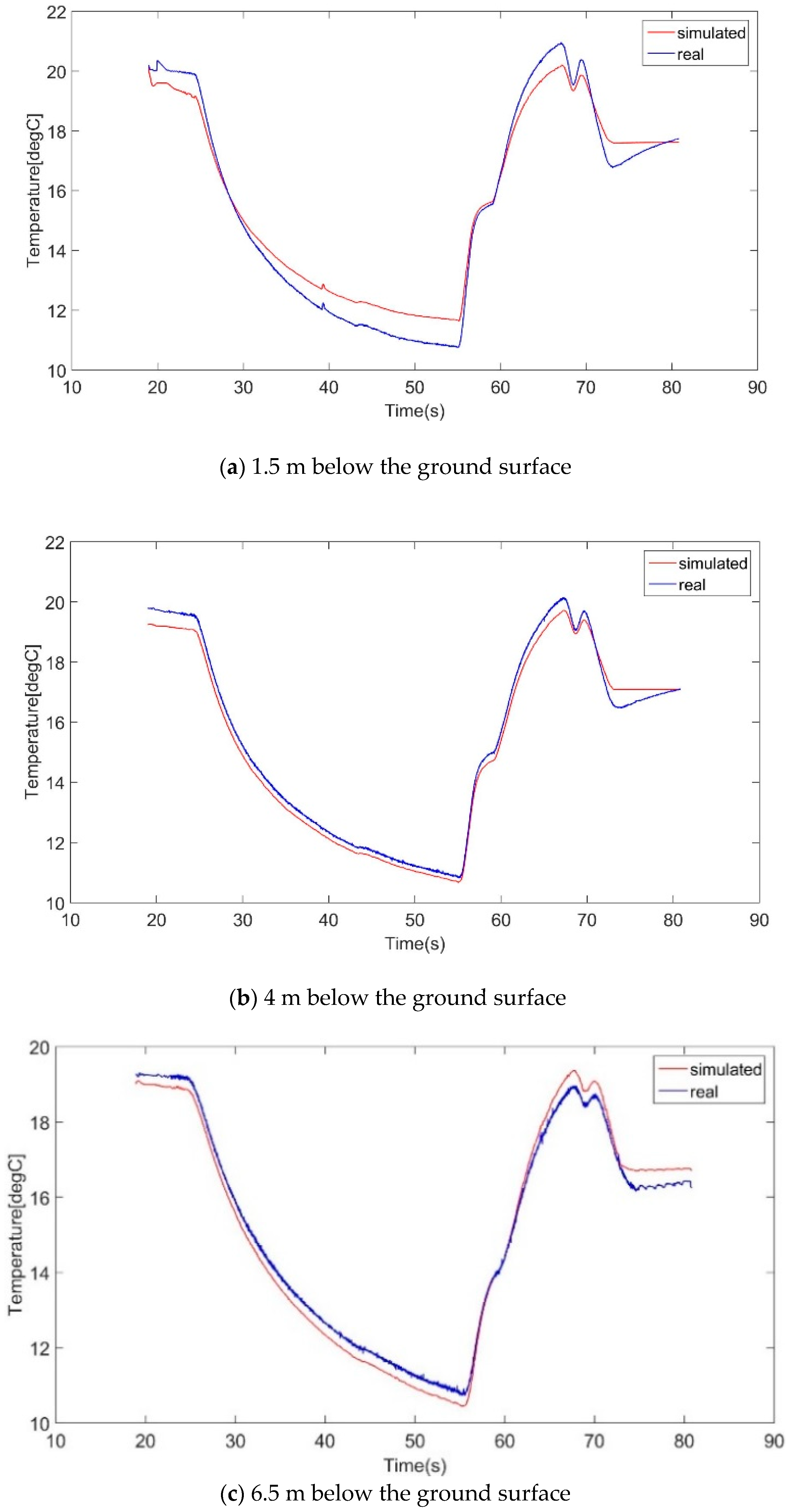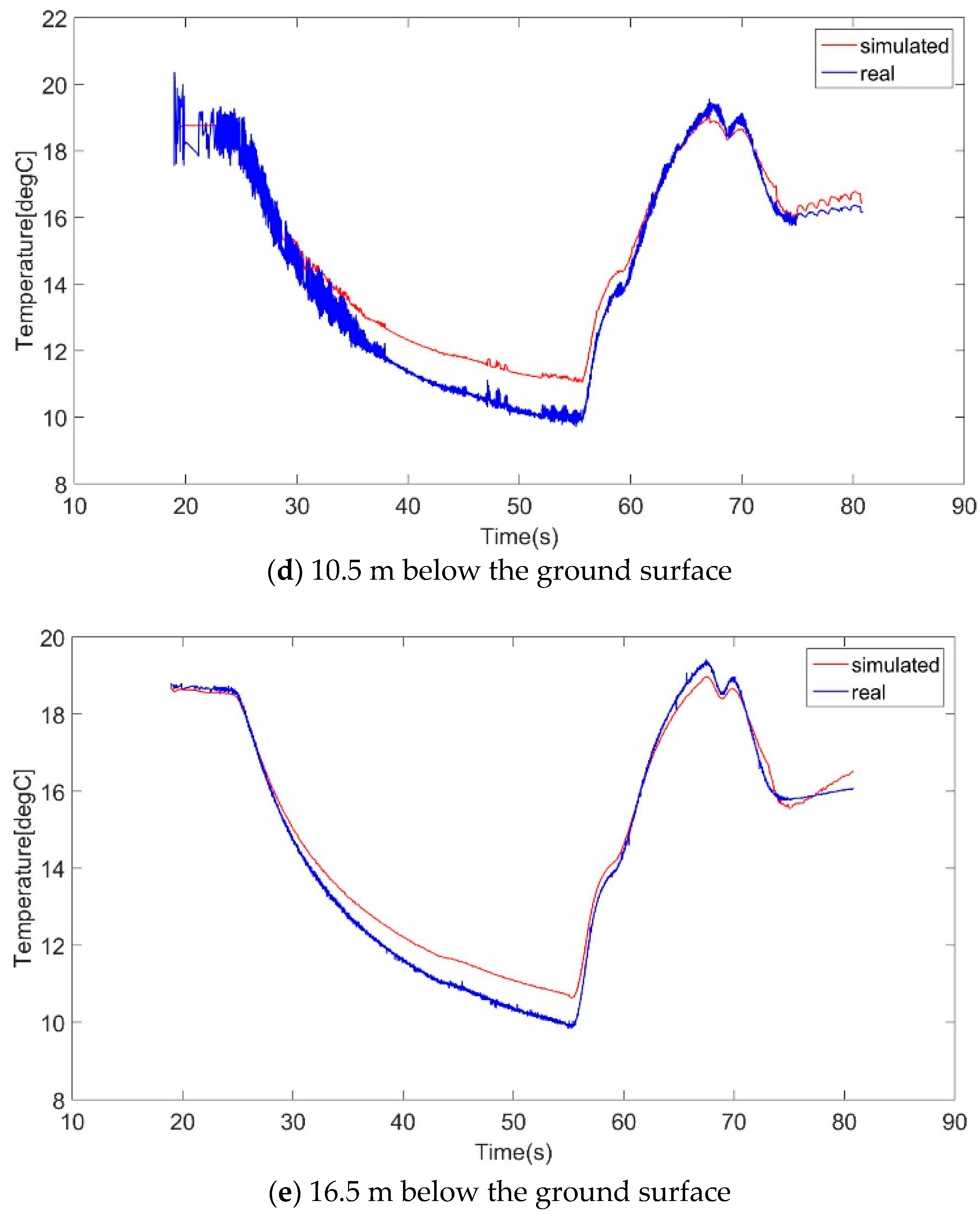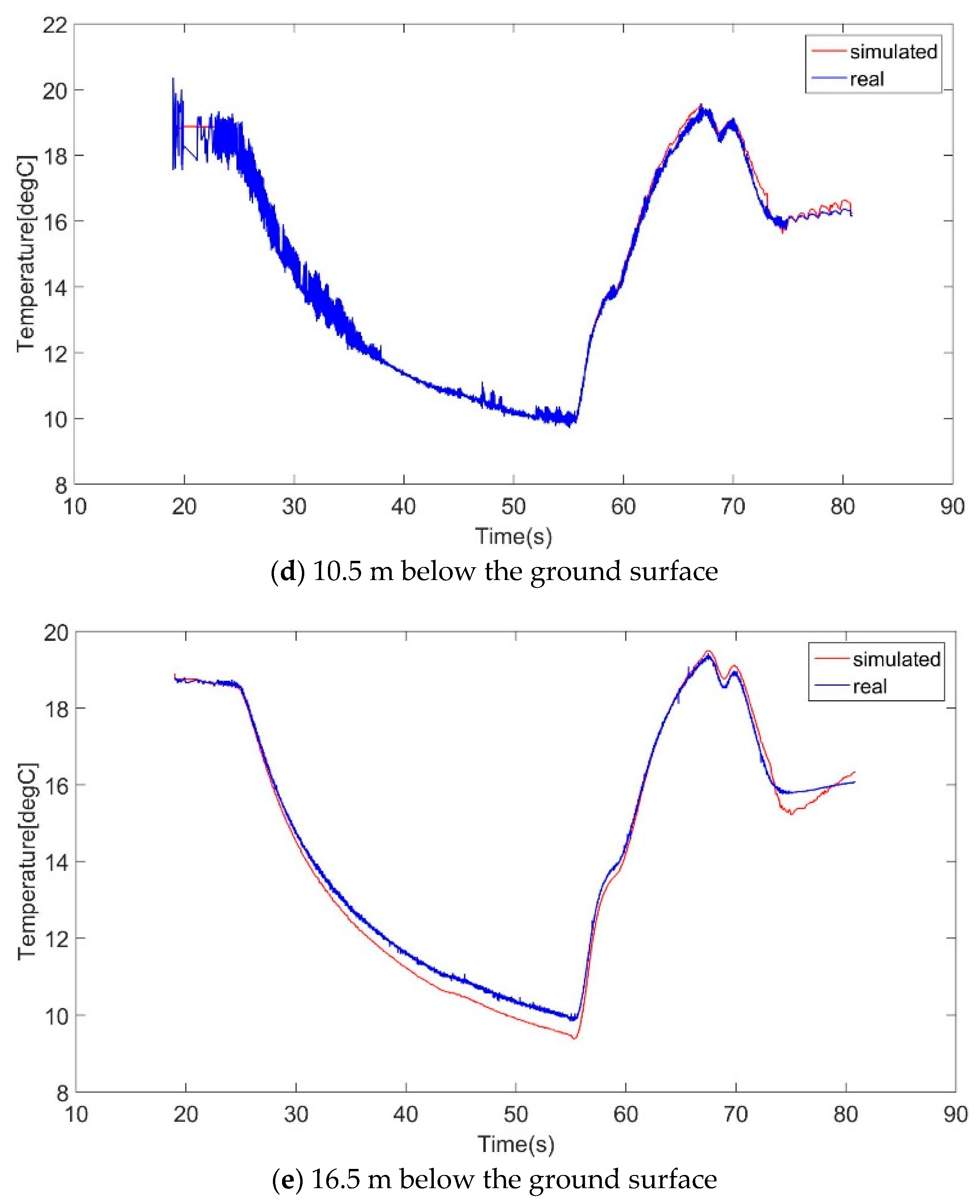Figure 9, Figure 10, Figure 11 and Figure 12 show the temperature profiles at the positions of the VWSGs located in the borehole, applying the conditions that h = 3, 4, 5, and 6 (Wm⁻²K⁻¹). If the simulated curve is lower than the monitored one in the cooling mode circle or higher than the monitored one in the heating mode circle, this means the heat transfer was more efficient than the real situation. Therefore, the value of h was overestimated, and hence the value was reduced.

From the Figure 9, Figure 10, Figure 11 and Figure 12, it can be seen that as the heat transfer coefficient rises, all the simulated curves exhibit the same trend of change. A large h applied at the concrete–soil interface can raise the peak temperature and pull down the valley. As expected, a larger value of h means that the heat flux is easily transferred to the ground; therefore, when the energy pile is working as a heat source/cold source, the nearby ground becomes hotter/colder.

According to the temperature profiles, the heat transfer coefficient value is complicated. It seems that the appropriate values are quite different from the different temperature values measured by the thermistors. For example, for VWSG1 the appropriate value of h is around 6 Wm⁻²K⁻¹, while for VWSG3 4 Wm⁻²K⁻¹ is already too large to fit the curves.

Table 3. Curve matching conditions for different h values at each VWSG.

	Cooled	Heated	h (Wm−2K−1)
VWSG1 (1.5 m depth)	- -	- -	h = 3
	- -	-	h = 4
	-	-	h = 5
	+	-	h = 6
VWSG2 (4 m depth)	-	-	h = 3
	+	-	h = 4
	+	O	h = 5
	+	+	h = 6
VWSG3 (6.5 m depth)	-	O	h = 3
	+	+	h = 4
	+	+	h = 5
	+ +	+ +	h = 6
VWSG4 (10.5 m depth)	- -	-	h = 3
	-	-	h = 4
	-	O	h = 5
	O	O	h = 6
VWSG5 (16.5 m depth)	-	-	h = 3
	-	-	h = 4
	O	O	h = 5
	+	O	h = 6

lists the curve matching conditions for different h values at each VWSG. The symbol “+” means that the h value is overestimated, and “+ +” means that the peak (valley) of the simulated curve is more than 2 °C higher (lower) than the monitored one. The symbol “-” means that the h value is underestimated, and “- -” means that the peak (valley) of the simulated curve is more than 2 °C lower (higher) than the monitored one. The symbol “O” means that the h value can make the two curves fit each other.

From Table 3, it can be concluded:

(1)

For VWSG 4 and 5, a consistent h value can be made to fit the whole curve. The fitting value is 6 Wm⁻²K⁻¹ for VWSG 4 and 5 Wm⁻²K⁻¹ for VWSG5.

(2)

For VWSG 1, 2, and 3, the approximate h values are different in the cooling and heating mode circles. In the cooling mode period, the approximate h value for both VWSG2 and 3 is 3–4 Wm⁻²K⁻¹, while this value in the heating mode circle is 5 Wm⁻²K⁻¹ for VWSG2 and 3 Wm⁻²K⁻¹ for VWSG3. For VWSG1 the curves match when h = 5–6 Wm⁻²K⁻¹ in the cooling mode and over 6 Wm⁻²K⁻¹ in the heating mode.

For the five groups of VWSGs, the hot/cold heat transfer coefficients are summarized in Table 3. For VWSG1 and 2, the heat transfer coefficient in the heating mode is larger than that of the cooling mode. For VWSG3 the result is the opposite, and the curves match with a higher h value in the cooling mode. For VWSG4 and 5 a single consistent heat transfer coefficient value works for both heating and cooling modes. The result of

Table 4. Hot/cold heat transfer coefficient comparisons.

	VWSG1	VWSG2	VWSG3	VWSG4	VWSG5
hhot vs. hcold	>	>	<	=	=

can partly support the assumption made in previous sections.

(a)

The VWSG 1 and 2 are close to the ground surface, and therefore the injected liquid has a large effect at these depths. VWSG 4 and 5 are buried deeper in the ground. At depths below 10 m, the injected heat (cold) has already been slightly lost. Therefore, the impact from the temperature of the liquid should be lower than the shallow positions. This may explain why for VWSG 4 and 5 the heat transfer coefficient difference between the hot mode and cold mode operations is quite small.

(b)

The pile diameter is not consistent. At the depth of VWSG 1 and 2, the pile diameter is 610 mm, while at the depth of VWSG 4 and 5 the diameter reduces to 550 mm. The heat-expansion and cold-contraction happen on the whole concrete body; therefore, the expansion/contraction is greater at the pile section with a larger diameter. As a result, the effect of expansion/contraction should be more significant at VWSG 1 and 2 than at VWSG 4 and 5.

(c)

There are different types of soil. At the depth of VWSG 1 and 2, the soil is “made ground”, while at the depth of VWSG 4 and 5 the pile is surrounded by London Clay. The material “made ground” is set to have a thermal conductivity of 2.5Wm⁻¹K⁻¹, while London Clay has a value of 1.7Wm⁻¹K⁻¹. This means the heat transfer efficiency is higher at the depth of VWSG 1 and 2 than VWSG 4 and 5. For the borehole that is some distance away from the test pile (0.5 m), the borehole temperature can be more sensitive at VWSG 1 and 2 than 4 and 5. This is another possible reason for the quite small h difference in VWSG 4 and 5 figures.

The result of VWSG3 is obviously against the hypothesis made in this chapter. However, it was noticed that VWSG3 acted different from all the other devices. It was the only VWSG to give a matched curve in the heating mode period with h = 3 Wm⁻²K⁻¹. For all the other instruments, the appropriate h for the hot mode was 5–6 Wm⁻²K⁻¹. It can be assumed that there are some special underground circumstances at the depth of VWSG3 (for example ground water flows) so that the heat transfer at that depth is abnormal compared to the whole pile.

6.2. The Shell Centre Case

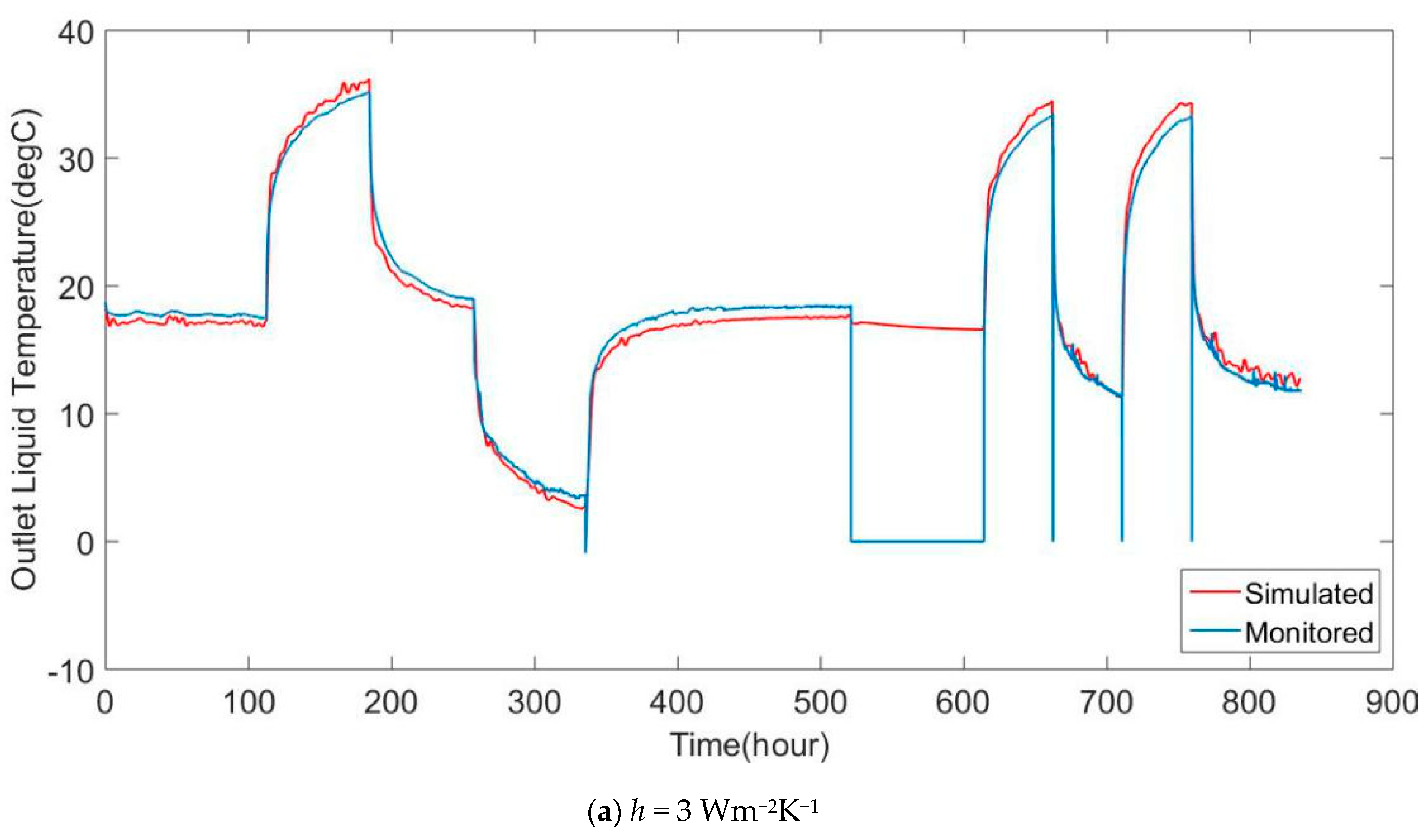
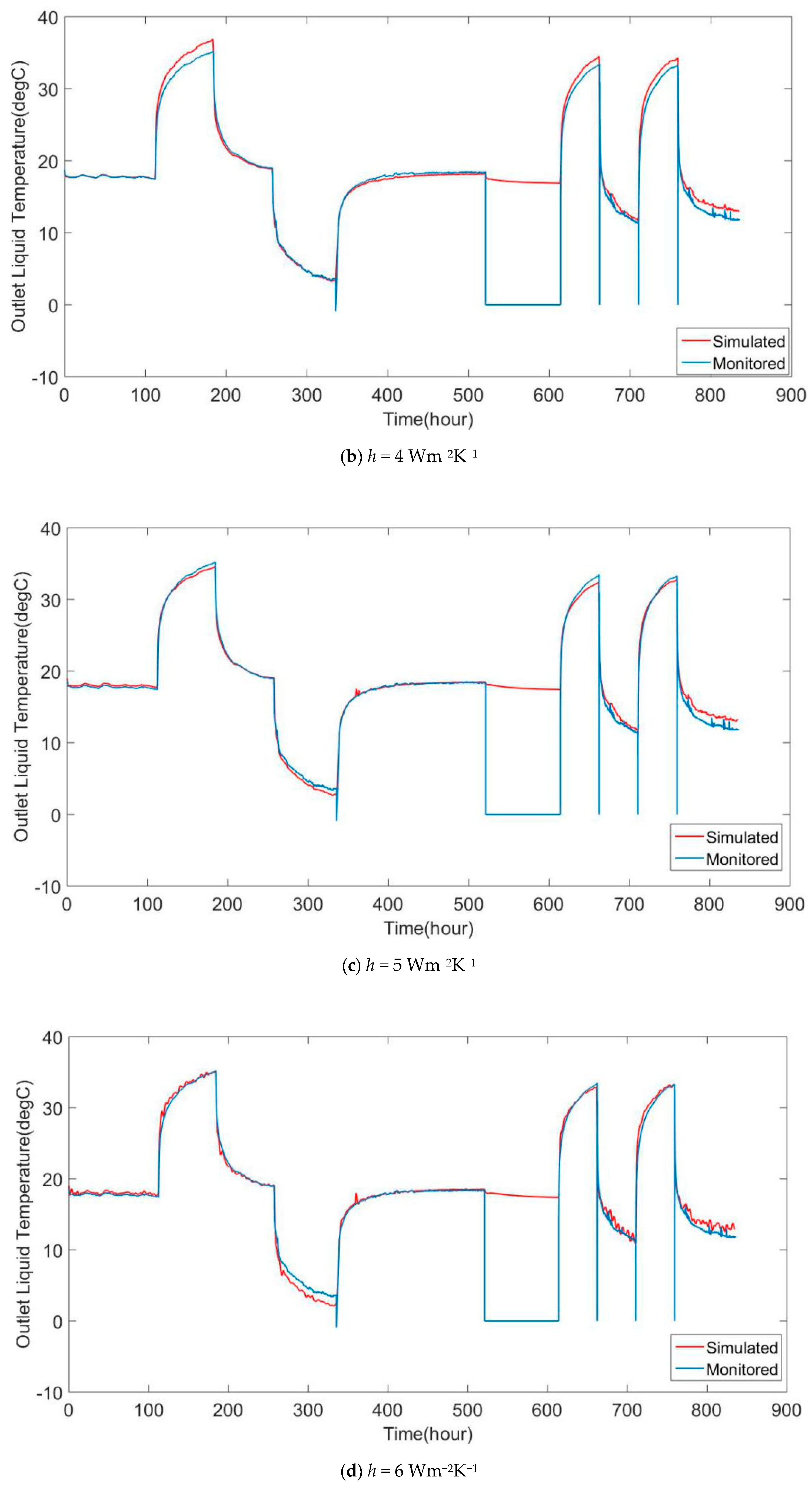
The heat transfer coefficient value across the concrete–soil interface was adjusted from 3 to 6 (Wm⁻²K⁻¹). Figure 13 shows that when h = 6 Wm⁻²K⁻¹, the curves match each other in the three heating mode sections, while h = 4 Wm⁻²K⁻¹ makes the curves matched at the cooling mode section. Therefore, the hypothesis described in Methodology is supported in this case.

In the Shell Centre project, the difference in values of h is smaller than that of the Lambeth College case. The most likely reason is the pile diameter. In the Lambeth College case, the pile diameter is 610 mm at the top and 550 mm for most of the depth. In the Shell Centre case, the borehole was enlarged to a diameter of 300 mm. As the temperature raises/drops, the pile body can expanse/contracts by a certain rate, therefore the large diameter pile can expanse/contract more movement than the small diameter ones. Therefore, the heat transfer coefficient difference in the Shell Centre is smaller than that of the Lambeth College one.

There is another probable reason for the smaller heating/cooling effect of Shell Centre case. Not as in Lambeth College case, there is no load on the pile of Shell Centre project. The load may cause side friction at the surface of the pile and the interface between the pile body and the ground could be tighter. A tighter interface can have a better h across it. Therefore, the impact from the heat extension and cold contraction could be larger as well. Further experiments could be developed to compare the h change with or without load on the pile.

Considering the variation of h on heat transfer is important to secure the stable performance of energy pile in the long-term. The influence of using an appropriate h value can get increased along with time because of the impact accumulation. Over a long time, the practical system yield can be different from the design value and the problem may come out regarding the uncertainty of energy supply. If the design supply is overestimated, there would be a waste on both the pile and the heat pump capacities. If the design supply is underestimated, the problem can be more severe as lack of energy supply would make people run the system for more operation hours. This action will not only reduce the system lifetime, but also increase the possibility of causing the thermal pollutions of the underground.

7. Conclusions

To develop a more detailed design for energy piles, the thermal resistance of pile should be considered. The heat transfer coefficient at the outer surface of the pile is an important component of the whole pile resistance. It was noticed that different heat transfer coefficient values should be applied as the operational mode switches for the energy pile. As the diameter of energy piles tends to be much greater than that of conventional borehole heat exchangers, the radial displacement due to thermal contraction and expansion of energy piles can be large. In the Lambeth College energy pile with a diameter of 550 mm, the difference of strain could be around 50 με when temperature variation between heating and cooling is around 20 degrees. This could be 25 μm movement at the concrete–soil interface. If a 25 μm small layer of air is located at the surface, which can lead to influence on the heat transfer behavior.

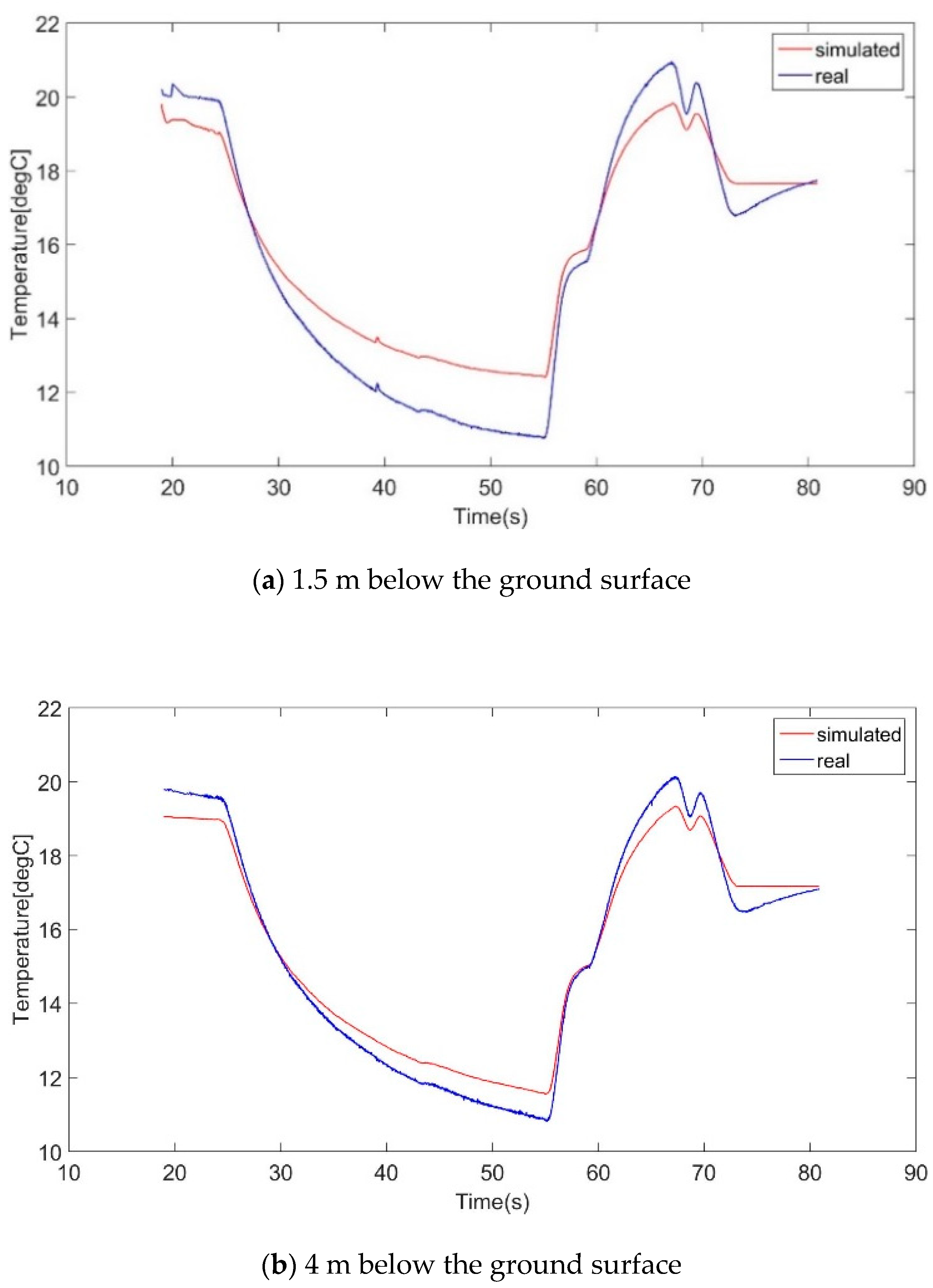
In the Lambeth College test, the ground temperature was directly monitored. The heat transfer coefficient from the pile to the ground was evaluated using a 3D FE model. Results at five different depths partly supported the hypothesis that the heat transfer coefficient in the heating mode is different from that in the cooling mode due to thermal expansion/contraction of the pile. At 1.5 m and 4 m, the heat transfer coefficient value (h) was 6 Wm⁻²K⁻¹ when the pile was heated, whereas it was 3–4 Wm⁻²K⁻¹ when the pile was cooled.

In the Shell Centre test, the proposed hypothesis is supported by the GSHP data. Numerical back-analysis was carried out based on the liquid temperature for a TRT trial. When fitting the model results to the monitored liquid temperatures, h = 4 Wm⁻²K⁻¹ gave a good fit when the pile was cooled, whereas h = 6 Wm⁻²K⁻¹ gave a good fit when the pile was heated. It can be noticed that the difference in the heat transfer coefficient for the Shell Centre energy pile was smaller than that for the Lambeth College one. The reason could be that the Shell Centre energy pile has a smaller diameter.

In summary, the back analysis of two energy pile cases illustrates that the heat transfer coefficient at the pile–soil interface can be different between the cooling mode and the heating mode. It is expected that the difference of h is influenced by a number of factors such as soil properties, concrete (grout) properties and the installation method. At present, the numerical studies of GSHPs always assumed that the concrete–soil interface is perfect to pass through the conductive heat transfer. To large size EGSs (e.g., energy piles with big diameter), this interface could lead to considerable impact, hence the determination of h value is of significance.