Machine Learning in Electrofacies Classification and Subsurface Lithology Interpretation: A Rough Set Theory Approach

Abstract

Initially, electrofacies were introduced to define a set of recorded well log responses in order to characterize and distinguish a bed from the other rock units, as an advancement to the conventional application of well logs. Well logs are continuous records of several physical properties of drilled rocks that can be related to different lithologies by experienced log analysts. This work is time consuming and likely to be imperfect because human analysis is subjective. Thus, any automated classification approach with high promptness and accuracy is very welcome by log analysts. One of the crucial requirements in petroleum engineering is to interpret a bed’s lithology, which can be done by grouping a formation into electrofacies. In the past, geophysical modelling, petro-physical analysis, artificial intelligence and several statistical method approaches have been implemented to interpret lithology. In this research, important well log features are selected by using the Extra Tree Classifier (ETC), and then five individual electrofacies are constructed by using the selected well log features. Finally, a rough set theory (RST)-based whitebox classification approach is proposed to classify the electrofacies by generating decision rules. These rules are later on used to determine the lithology classes and we found that RST is beneficial for performing data mining tasks such as data classification and rule extraction from uncertain and vague well log datasets. A comparison study is also provided, where we use support vector machine (SVM), deep learning based on feedforward multilayer perceptron (MLP) and random forest classifier (RFC) to compare the electrofacies classification accuracy.

1. Introduction

Lithology refers to the composition or type of rock in the Earth’s subsurface. The term lithology is used as a gross description of a rock layer in the subsurface and uses familiar names, including sandstone, claystone (clay), shale (mudrock), siltstone, and so forth. In earth science, subsurface properties such as lithology identification have always been among the basic problems. A number of methods in lithology interpretation have been proposed by researchers. Conventional methods that employ seismic data for the estimation of reservoir lithology properties consist of finding a physical relationship between the properties to be identified and the seismic attributes and then employ that attribute over the entire seismic dataset in order to predict the target properties. Many seismic datasets are inundated with noise values, e.g., sensor noisy responses or equipment mismeasurements. In some cases, when the functional relationships between the attributes and the target properties can be found, the physical foundation is not often clear or understandable. In contrast, inferring lithology properties from the recorded well logs is much more reliable but economically expensive, challenging and time consuming. The lithology of a layer can also be identified by drilling holes, although this method often does not provide exact information. We can also obtain results from recorded continuous cores that are very expensive and might be unprofitable. The lithology can also be interpreted by geophysical inversion and geophysical modelling methods. The interpretation of lithology using electrofacies from well logs multi-attribute data has become one of the most prominent techniques used by several sectors of petroleum engineering, including geological studies for reservoir characterization, although petrophysical well logs contain uncertainty and noise.

Clustering the recorded well logs is done to find similar or dissimilar patterns among the well log values in the multivariate space with an aim to group them together into individual classes called electrofacies [1]. Electrofacies have a unique set of log responses that can separate the material properties of the rocks and fluids contained in the volume recorded using the well-logging tools. These identified electrofacies can interpret and reflect the lithologic, diagenetic and hydrologic characteristics of an uncored well. By applying the additional information such as geological insight or core observations, the identified electrofacies (EF) clusters can be calibrated to ensure their interpretable geological meaning, and for this, the electrofacies classification process needs to be explained efficiently. Ideally, for defining electrofacies, there is no exact method. The electrofacies can be defined on the basis of standard well-log data, such as neutron porosity, gamma ray, resistivity, bulk density, caliper log, photoelectric effect, and so forth. Furthermore, they can often be associated to one or more lithofacies. Conventionally, lithofacies have been identified manually, depending on the core description and their relation to well-logs. The usual prerequisites are that the electrofacies should be defined from a reliable log set of petrophysical measurements and the similarities or dissimilarities among the down-hole intervals needs to be explained quantitatively from the sample log responses.

This research proposes:

• An extra trees classifier (ETC)-based well log feature selection method.
• A critical “whitebox” approach using the rule induction algorithm of rough set theory (RST) towards classifying the electrofacies which have been constructed by the non-hierarchical K-means clustering algorithm.
• A unique method to determine the lithology from the electrofacies by employing the RST rules.

RST is a machine learning tool which performs granular computation in a vague idea (set) based on two vivid sets of concepts: lower approximations and upper approximations. RST requires only the provided dataset to employ the granular methodological computations [2]. Among the numerous advantages of RST [3,4], some are shown below.

• Provides effective algorithms to discover patterns in the provided dataset.
• Constructs a nominal dataset named data reduction and, thus, shows the significance of data.
• Generates a set of decision rules from the data samples which are easily interpretable.

The remainder of the paper is organized as follows. Section 2 contains the problem and the background. In Section 3 the experimental steps to select important features, construct and classify the electrofacies, and interpret lithology are described. In Section 4 a comparison study is provided. Section 5 contains the discussion and concludes the paper.

2. Problem and the Background

A number of methods have been used for solving lithology classification and interpretation problems, such as cross plot interpretation and statistical analysis based on histogram plotting [5], support vector machine (SVM) using traditional wireline well logs [6], fuzzy-logics (FL) for association analysis, neural networks and multivariable statistical methodologies [7], artificial intelligence approaches and multivariate statistical analysis [8], hybrid NN methods [9], self organized map (SOM) [10], FL methods [11], artificial neural network (ANN) methods [12,13], lithology classification from seismic tomography [14], multi-agent collaborative learning architecture approaches [15], random forest [16,17], generative adversarial network [18] and multivariate statistical methods [19].

Numerous mathematical approaches have been introduced recently to automate the process of identifying and classifying electrofacies. In several researches the general information about lithology and rock properties changes are extracted from the electrofacies for pattern recognition [20,21,22]. The researches mainly consist of applying discriminant analysis, principal components analysis (PCA), and cluster analysis [20,21].

To classify electrofacies, numerous other approaches are shown in the literature [22,23,24,25,26]. The majority of the available commercial software packages and approaches for subsurface modeling include electrofacies functions. However, the explanations of how these functions generate the results are rarely explained and the processes operate as “blackboxes.” In [27], the feedforward neural network and clustering are used for the determination and classification of electrofacies, which are also black-box approaches.

The performance of the ANN and FL methods are superior compared with statistical methods [6,7,12,13,19,28]. SOM methods provide better results in lithology classification compared to other machine learning techniques [29]. Other kinds of NN are faster than probabilistic neural networks (PNN), because PNN involves more computational steps [19].

Recently, rule-based whitebox classification modules such as RST has been used in several related areas for solving classification problem analysis [30,31]. Touhid at al. [32] have used non-deterministic apriori rules to identify lithology classes directly from well logs.

3. Experimental Steps

3.1. Feature Selection

Ideally, a lot of well log features are available for constructing electrofacies. Depending on the resolution and responses to the properties of interest, prominent features or attributes can be selected. In this study, we use Extra Trees Classifier (ETC) to select the prominent features from 28 well log features. The Extra Trees Classifier, also known as the Extremely Randomized Trees Classifier, is an extension to the random forest classifier section of ensemble learning technique which combines the outputs of numerous de-correlated decision trees together as a “forest” for calculating its classification result [33].

During the construction of the forest, each feature is descendingly ordered on the basis of the mathematical criterion (Gini Index, Information Gain Entropy) used in the decision of feature of split that is recorded during the calculation. We have chosen Gini Index over Information Gain Entropy, since Gini Index doesn not require to compute logarithmic functions, which Information Gain Entropy does, making it computationally expensive [34,35]. In ETC-based feature selection, based on the Gini Importance [36], the user can select the important k number of features according to the application criteria. Although in electrofacies classification, the number of independent feature can be arbitrary. 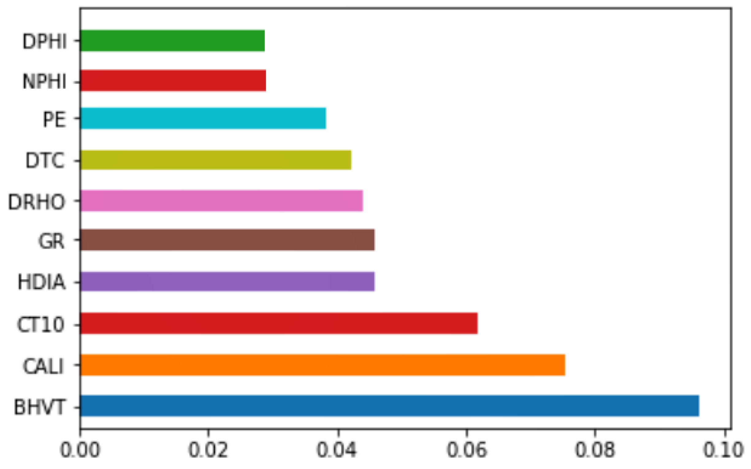Nashawi and Malallah [37] and Edyta Puskarczyk [18] both have used six well log features but not the same feature set to construct the electofacies, whereas Kumar and Kishore [27] used four well log features. In general, the purpose of reducing the number of features is to reduce overfitting and training time and to lessen misleading data to improve accuracy. We have considered k = 10 to get the 10 most prominent features out of 28 well log features in the original well log dataset for constructing and classifying the electrofacies classes. In the process of selecting features, lithology classes are used as the dependent feature, since the constructed electrofacies classes will be used for interpreting lithology in the extension of the work. In Figure 1, the calculated feature importance is shown.

Table 1. Summaries of the selected well log attributes.

	GR	NPHI	DRHO	PE	DPHI
Attribute Name	Gamma Ray	Neutron Porosity	Density Correlation	Photoelectric Effect	Density Porosity
Unit	.api	.decp	.g/cc	.none	.decp
Min.	46.49	0.1053	−0.05	0.5105	0.081
Mean	140.85	0.2942	0.02471	1.8684	0.254
Max.	385.89	1.2316	0.3244	3.7343	0.8082
	CT10	CALI	BHVT	DTC	HDIA
Attribute Name	Conductivity	Caliper	Borehole Volume	Compressional Sonic	Hole Diameter
Unit	.mmo/m	.in	.m${}^3$	.uspf	.in
Min.	113.9	5.297	0.4481	60.81	5.297
Mean	1240.4	5.863	2.0633	101.69	5.863
Max.	9215.5	7.58	4.265	159.61	7.58

below includes the description of the selected attributes and their summaries:

3.2. Electrofacies Construction

3.2.1. Clustering the Logs

The purpose of clustering is to classify a dataset into several groups which are externally isolated and internally homogeneous on the basis of a measure of similarity and dissimilarity among the groups. Since electrofacies are defined empirically, the number of electrofacies classes is arbitrary. Usually, the number of defined electrofacies depends on the number of log properties used in the system and the joint characteristics of the statistical distributions of the log readings [38]. It also represents the target of electrofacies classification and the way in where the final categorization will be interpreted and used. In our experiment, we selected five electrofacies classes to be constructed by a non hierarchical k-means clustering algorithm, which is one of the most popular and widespread partitioning clustering algorithms because of its superior feasibility and efficiency in dealing with a large amount of data [39]. Several studies have suggested and used k-means clustering for constructing electrofacies [18,27].

K-means clustering [40] is a distance-based clustering method for finding clusters and cluster centres in a set of unlabelled data. This is a fairly tried and tested method in which the goal is to group points that are ‘similar’ (based on distance) together. This is done so by regarding the centre of data points as the centre of the corresponding clusters (centroids). The core idea is to update the cluster centroid by iterative computation, and the iterative process will be continued until some convergence criteria are met.

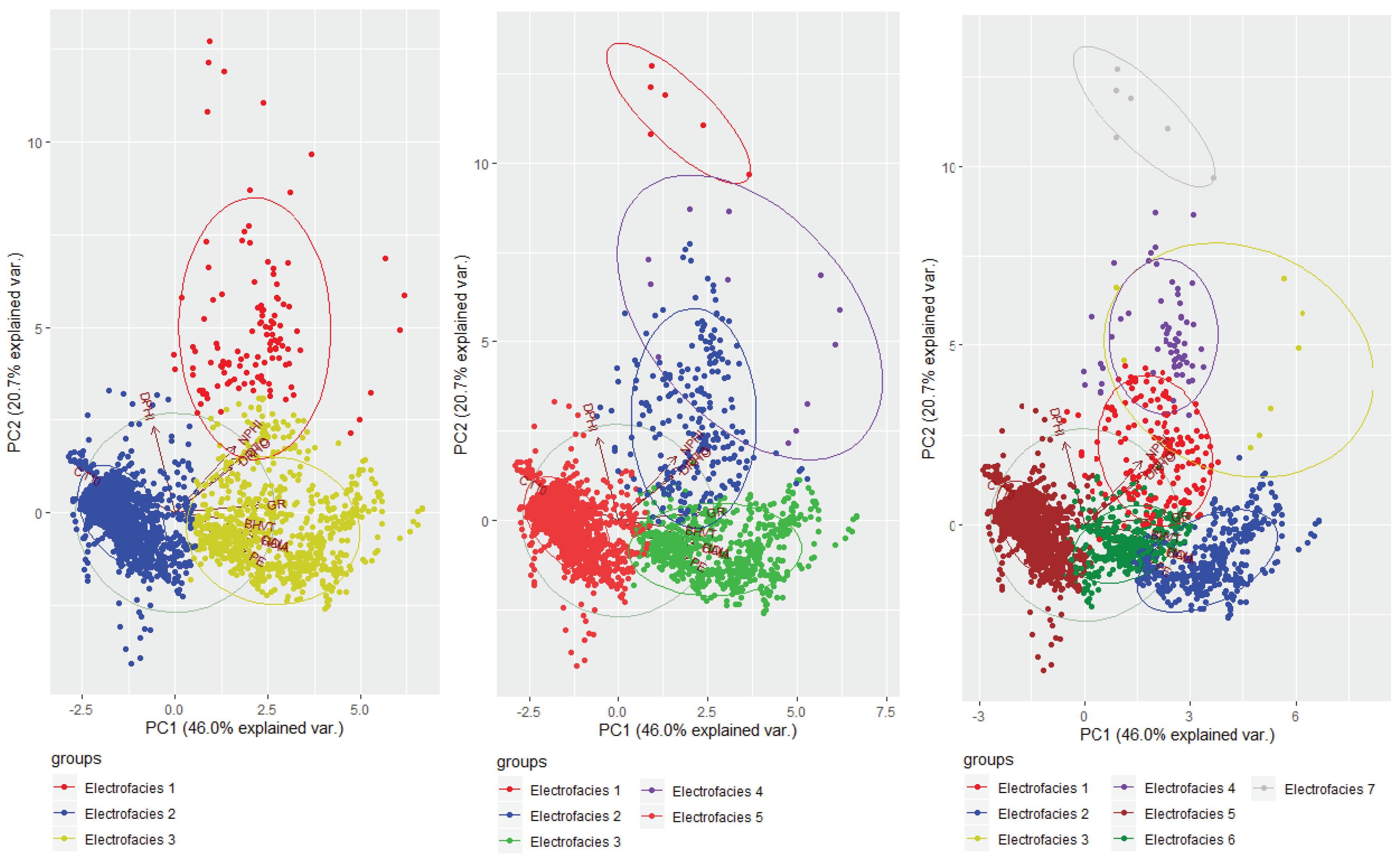
To get a proper distribution of the dataset, the well log values of all the independent features were standardized to z-scores. The cluster classes are illustrated in Figure 2.

3.2.2. Visualizing the Clusters

For related problems and to generate principal component values for electrofacies classification, several studies has been done using Principal Component Aanalysis (PCA) [41]. PCA is usually used for reducing the dimensionality of the data and for summarizing and visualizing the data efficiently without information. In our research, PCA is done to visualize the distribution of the logs according to the electrofacies classes defined by the clustering algorithm and for building the classification model using RST, the raw values (not the component values) from the logs have been used. For the input of the PCA analysis, standardized values of logs are used. From Figure 2 it is clear that considering five electrofacies classes, the electrofacies classes follow proper disjoint distribution which is projected by the bi-plot generated by principal component 1 (PC1) and principal component 2 (PC2).

3.3. EF Classification Module Using RST Rule Induction

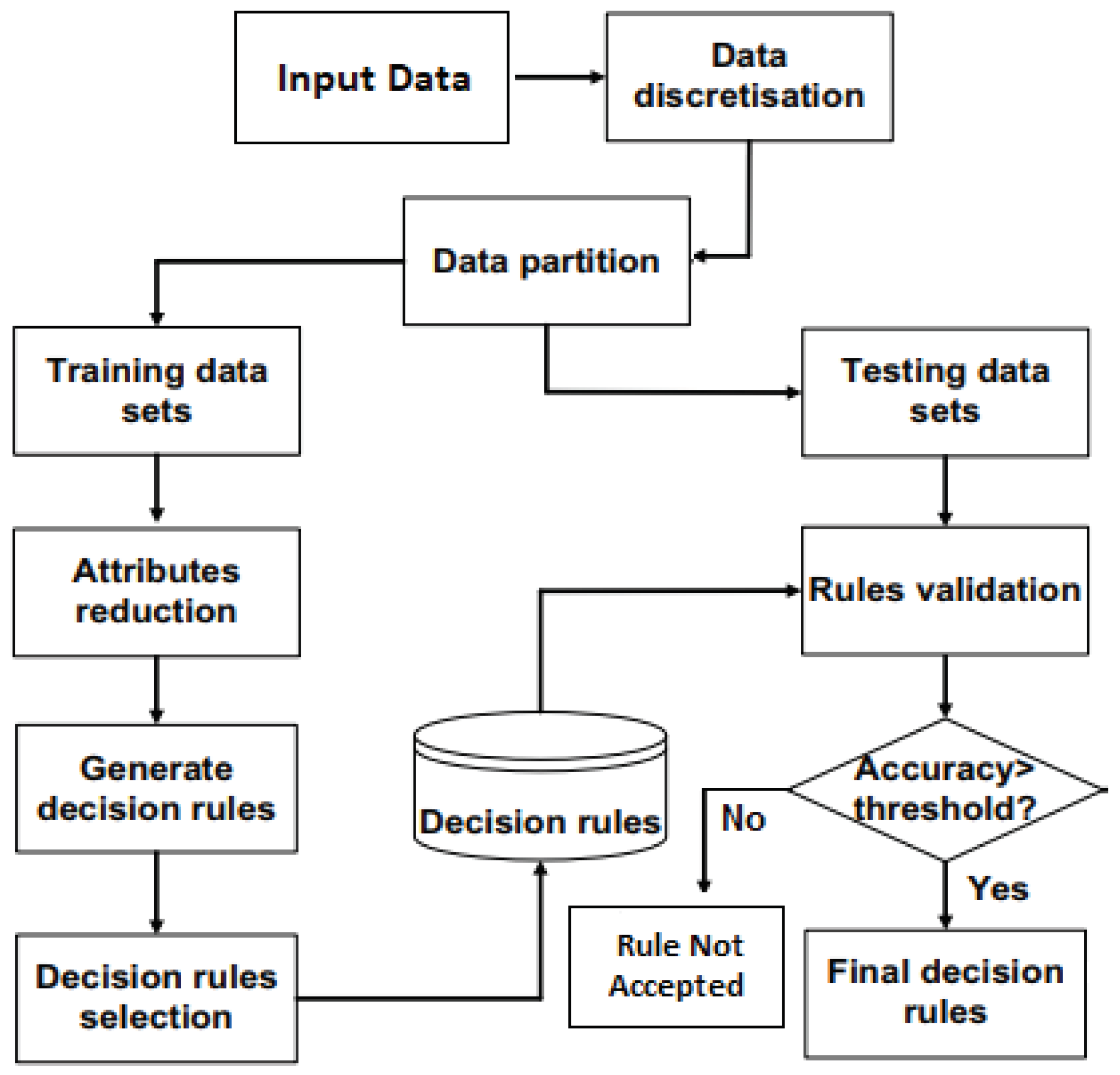
Although the k-means clustering algorithm classifies the well log responses into an arbitrary number of electrofacies, it is unable to provide a posterior classifier, which means it cannot generate classification rules or mathematical functions which can be used for assigning new log readings to the electrofacies categories that are being constructed. Hence, an addition is needed to take care of this issue. Rough set theory-based rule induction can be used to generate a set of rules that will define the possible electrofacies clusters separately in terms of rules in effect.

To implement RST, these following computational steps are required (as shown in Figure 3):

3.3.1. Data Preparation

In this step, the main dataset is constructed by using the selected well log features and the elecrofacies class information for each objects as constructed in Section 3.2. The number of samples or objects in the main dataset is 5560. We divided the main dataset into two subsets, training dataset that we have denoted as DTr (70% or 3892 samples) and testing dataset that we have denoted as DTst (30% or 1668 samples). The training dataset, DTr was used to extract rules by using the RST rule induction methodology, and for prediction, the testing dataset, DTst was used. Since the data values in DTr and DTst are continuous, and RST requires the training data values to be discrete, some data prepossessing is done in Section 3.3.2.

3.3.2. Binning or Discretization

In this step, the continuous explanatory attribute values of the training dataset are discretized using the global discernibility heuristic method. Usually, the most used binning methods are equal length binning and equal frequency binning. Global discernibility heuristic binning is a supervised discretization method based on the maximum discernibility heuristic. It is used for computing globally semi-optimal cuts using the maximum discernibility heuristic [42]. However, the decision attribute electrofacies does not need to be discretized, since it is already a categorical variable. In

Table 2. Cut points of the attributes.

Cut Point No.	GR	NPHI	DRHO	PE	DPHI	CT10	CALI	BHVT	HDIA	DTC
1	[-Inf, 170]	[-Inf, 0.241]	[-Inf, 0.0279]	[-Inf, 1.48]	[-Inf, 0.294]	[-Inf, 342]	[-Inf, 6.05]	[-Inf, 1.54]	[-Inf, 5.60]	[-Inf, 107]
2	(170, 208]	(0.241, 0.327]	(0.0279, 0.0969]	(1.48, 2.27]	[-Inf, 0.294]	(342, 370]	(6.05, 6.3]	(1.54, 2.78]	(5.60, 6.51]	(107, Inf]
3	(208, Inf]	(0.327, 0.336]	(0.0969, Inf]	(2.27, Inf]	(0.294, Inf]	(370, 886]	(6.3, Inf]	(2.78, 3.7]	(6.51, Inf]
4		(0.336, 0.345]				(886, Inf]		(3.7, Inf]
5		(0.345, Inf]

the cut points of all the attributes are shown.

3.3.3. Generation of Reduct

Cores and reducts are generated in this step and the training set DTr is used. After the execution of this step, a minimal subset is found which consists of the features which subset still provides the same quality of information that were present in the main dataset [30].

3.3.4. Generation of Rules

In this step, DTr is used for extracting rules using RST Rule Induction algorithm [30]. In this step the support and confidence of the rules are also counted. The RST rule R can be represented as, $R:(b{x}_1$ = $K{x}_1)\wedge (b{x}_2=K{x}_2)$, $\wedge \dots \wedge (b{x}_n=K{x}_n)\to (d=K)$ where, $b{x}_y$ and $K{x}_y$ denote the independent features and the their values respectively. The left hand side of the rule R is the set of feature value sets which is the condition part and denoted as $cond\left(R\right)$, and the right hand side of R is referred as the decision part, $dec\left(R\right)$. In short, a rule in RST is expressed as, IF $cond\left(R\right)$ THEN $dec\left(R\right)$. By following the RST methodology, 66 rules are generated as shown in

Table 3. Rules generated by Rough Set Theory.

Rule					IF						THEN	Support	Laplace
No.	GR	NPHI	DRHO	PE	DPHI	CT10	CALI	BHVT	HDIA	DTC	EF	Size	Value
1	1									1	5	982	0.996
2			1			3			1	1	5	923	0.996
3		1			4			2			5	258	0.985
4			1	1				1	1		5	117	0.967
5					2			1		1	5	77	0.951
6	1					3		2			5	382	0.990
7	2		2					2		1	5	11	0.750
8			2			3	1				5	47	0.923
9			1		3		1		1		5	311	0.987
10	1				4		2				5	56	0.934
11		1		2					2	1	5	436	0.991
12	2		3		3				3		5	3	0.500
13			2			3		3			5	10	0.733
14			1	2	4						5	250	0.984
15	3				3	3					5	26	0.871
16	1			1	3		1				5	73	0.949
17					4	2		2	3		5	74	0.949
18			2		4				1		5	27	0.875
19	2			2				2			5	23	0.857
20			1	2			1				5	398	0.990
21					3	2		2			5	24	0.862
22	2					3		3			5	1	0.333
23	2		4			2					5	3	0.500
24				4				3			3	267	0.985
25	3	2	1	4							3	113	0.966
26		2			2			3			3	255	0.985
27					3	1	2	3			3	88	0.957
28		1			2					2	3	37	0.905
29				4				2		2	3	28	0.879
30				3			1	3			3	29	0.882
31					3	2		3			3	10	0.733
32				3				3		1	3	33	0.895
33			3		2					2	3	51	0.929
34	3	2		2	2						3	6	0.636
35			3		2			2			3	12	0.765
36		1	4					2	2		3	3	0.500
37			1	3	4					2	3	2	0.429
38				2			1	3		2	3	7	0.667
39			4		1						3	2	0.429
40			1	2	3			3			3	17	0.818
41	3		2	4		1					3	78	0.952
42			2		2			1		2	3	1	0.333
43		2		3	3	3				2	3	1	0.333
44	1		1		4		1	3			3	1	0.333
45	3	2	1		2						3	108	0.965
46	3		3		3	1	2				3	12	0.765
47			4					1	2	2	2	65	0.943
48			4	1							2	47	0.923
49			4	3			2	2			2	6	0.636
50	3		4					1			2	80	0.953
51			4	2	4						2	5	0.600
52					5	1					2	60	0.939
53		2	4	3				2			2	9	0.714
54			4	4	3					1	2	8	0.692
55			3		4	1		1			2	4	0.556
56			3	3		1	1		2	2	2	2	0.429
57	3		3		3		1	1			2	1	0.333
58			4	2					1	2	2	12	0.765
59			3		4	3		2			2	2	0.429
60			3	1				1		2	2	1	0.333
61					3	2		1		2	2	1	0.333
62			3			3	2	2			4	2	0.429
63			3	4		3					4	2	0.429
64	3		3		5	2					4	1	0.333
65			3	2			2	1	1		1	3	0.500
66			3	3	5						1	1	0.333

below:

3.3.5. Validation of the Generated Rules

In this step, the validation of the reduced rules is performed, which turns the rules into final decision rules by incorporating the threshold accuracy or confidance, which is also denoted as Laplace. Confidence or Laplace is an indication of how often the rule has been found to be true. (Laplace > 0.33 or 33% for our experiment). If this threshold is raised, the number of rules to solve the problem decreases, which causes the overall prediction accuracy to be lesser. The process is shown in Figure 3.

3.4. Calculating Lithology Prediction Accuracy for Model Evaluation

The decision rules that we found from the experiment by using the training dataset DTr are applied to DTr itself and to the testing dataset DTst to calculate the Training and Testing prediction accuracy (PA). The prediction accuracy (PA) is calculated by employing the decision rules.

$$PA=\frac{No.ofcorrectlyclassifiedinstances}{No.ofinstancesinthedataset}\times 100\%$$

(1)

From our experiment, the result shows that the module has a PA of 98.08% for the testing dataset, DTr, which means the model has a 1.12% misclassification rate which ensures the reliability of the RST rules to distinguish the electrofacies classes. In

Table 4. Confusion matrices for training and testing sets.

Sample	Observed	Predicted
		EF 1	EF 2	EF 3	EF 4	EF 5	Correct (%)
	EF 1	245	2	3	0	3	96.84%
	EF 2	2	1213	0	0	0	99.84%
Training	EF 3	1	0	236	0	2	98.74%
	EF 4	0	1	0	5	1	71.43%
	EF 5	4	5	0	0	191	95.50%
	Overall (%)	13.17%	63.79%	12.49%	0.26%	10.29%	98.75%
	EF 1	120	2	3	0	1	95.24%
	EF 2	1	518	1	0	2	99.23%
Testing	EF 3	2	0	106	0	0	98.15%
	EF 4	0	0	0	6	3	66.67%
	EF 5	0	0	0	0	68	98.55%
	Overall (%)	14.75%	62.59%	13.19%	0.72%	8.75%	98.08%

the classification results for DTr and DTst are shown.

3.5. Lithologic Description of the Electrofacies

An empirical interpretation of the identified electrofacies has been made by comparing the electrofacies classes to core descriptions for the well in which extensive set of cores were taken. The core descriptions were written by different geologists who may have emphasized different aspects of the rock or who used different definitions of their descriptive terms and hence, the interpretations are basically somewhat ambiguous, because

Table 5. Number of samples in each electrofacies according to the lithology classes.

Lithology Classes	EF 1	EF 2	EF 3	EF 4	EF 5	Total in 5 EFs
Claystone	21	3	106	0	16	146
Mudstone	66	86	89	3	92	336
Siltston	0	23	0	13	0	36
Sandstone	94	1506	18	0	83	1701
Sandy Mudstone	84	42	107	0	45	278
Sandy Siltstone	0	21	9	0	9	39
Silty sandstone	41	51	6	0	14	112
Silty Mudstone	0	0	0	0	10	10
Muddy Sandstone	69	0	12	0	0	81
Granulestone	3	5	0	0	0	8
Total in 10 Lithology Classes	378	1737	347	16	269	2747

represents an amalgam of the contribution of the lithology classes in forming the identified electrofacies.

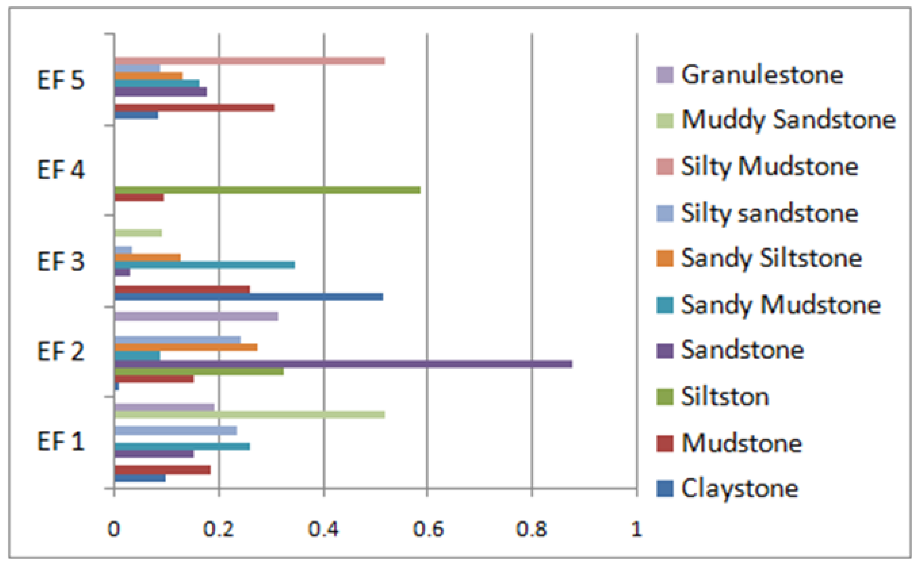
Based on the information in Table 5, the lithologic contributions in each electrofacies are represented in Figure 4.

The lithologic descriptions of the electrofacies can be obtained on the basis of the information in Table 5 and Figure 4, which are shown in

Table 6. The lithologic descriptions of the electrofacies.

	Very High	Medium	Low	Very Low
EF 1	Muddy Sandstone	Sandy Mudstone and Granulestone	Silty sandstone and Mudstone	Claystone, Sandstone
EF 2	Sandstone and Granulestone	Siltstone	Sandy Siltstone and Silty Sandstone	Mudstone and Sandy Mudstone.
EF 3	Claystone	Sandy Mudstone	Mudstone and Muddy Sandstone	Sandy Siltstone.
EF 4	Siltston
EF 5	Silty Mudstone	Mudstone	Sandy Mudstone	Claystone, Sandy Siltstone and Silty Sandstone

below:

From the preceding table it is vivid that,

• Electrofacies 1: Mainly consists of Muddy Sandstone. However it also consists Sandy Mudstone, Granulestone, Silty Sandstone, Mudstone, Claystone and Sandstone, as shown in Table 6.
• Electrofacies 2: Mainly represents Sandstone. However, it also consists Granulestone, Siltstone, Sandy Siltstone, Silty Sandstone, Mudstone and Sandy Mudstone.
• Electrofacies 3: Mainly Represents Claystone. However it also consists Sandy Mudstone, Mudstone, Muddy Sandstone and Sandy Siltstone.
• Electrofacies 4: Electrofacies 4 represents Siltston.
• Electrofacies 5: Mainly represents Silty Mudstone. However, it also consists Mudstone, Sandy Mudstone, Claystone, Sandy Siltstone and Silty Sandstone.

At this point, the classification rules generated from Section 3.3 can describe the electrofacies classes as well as the lithologic descriptions of the well.

4. Comparison Study

For comparison, we have used three other techniques such as SVM, deep learning and RFC to obtain the accuracy for classifying the electrofacies classes:

4.1. Support Vector Machine (SVM)

SVM is a machine learning tool proposed by Vladmir Vapnik in 1996 [43] that has been used for 20 years to solve several problems, including lithology and electrofacies classification [29,43,44]. In SVM, the algorithm finds a hyper-plane in an M-dimensional space where M is the number of features that distinctly classifies the data values. Hyper-planes are actually the boundaries of decision that make the classifications the data points. Data points falling on any side of the hyperplane are considered to be in separate classes [43]. Data points that are closer to the hyperplane can influence the orientation and position of the hyper-plane, and they are called support vectors. To examine how SVM performs, the same datasets that we used for RST were used. For training and testing the datasets, the same training and testing ratio (70:30) was selected. We implemented nonlinear type-1 SVM and the following settings were selected:

• Kernel = radial basis function kernel
• C value = 1
• Cache size = 200
• Gamma = auto deprecated

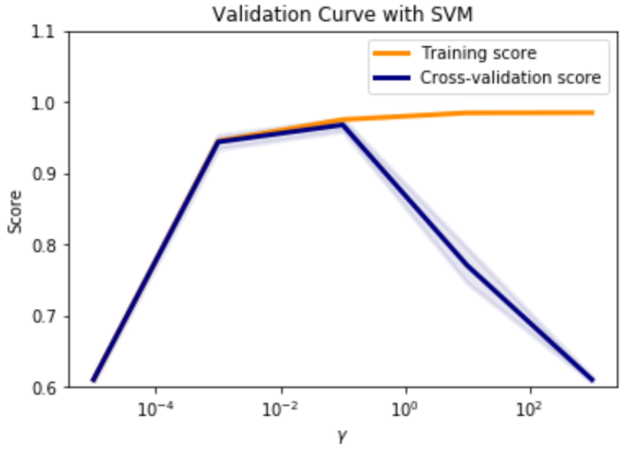
Where C is the regularization tradeoff parameter for the soft margin cost function that controls the effect of each individual support vector. The gamma parameter is used as a similarity measure between two points. A small gamma value defines a Gaussian function with a large variance, where two points can be considered similar although they are away from each other. On the contrary, a large gamma value creates a Gaussian function with small variance, where two points in close distance are considered similar.

In Figure 5, along the y-axis, the prediction scores for training and cross-validation are illustrated with respect to the change in gamma values in x-axis. In

Table 7. Training and testing accuracies for RST and other methods and their percent difference with RST.

	RST	SVM		Deep Learning		RFC
	Accuracy	Accuracy	PD (%)	Accuracy	PD (%)	Accuracy	PD (%)
Training	0.9875	0.9833	−0.0043	0.9806	−0.0070	0.9868	−0.0007
Validation	0.9808	0.9798	−0.0010	0.9794	−0.0014	0.9794	−0.0014

, the training and the cross validation scores are shown (best result achieved when $\gamma ={10}^{-1}$).

4.2. Deep Learning

Over the years, ANN has been used for solving data pattern recognition and classification problems [45,46]. ANN methods have a noticeable ability to construct a complex mapping between nonlinearly coupled input and output data. A deep neural network (DNN), also known as deep learning is an artificial neural network (ANN) having several hidden layers and that can solve problems more efficiently and find very complex relationships among the attributes using multiple layers in between the input and output layers. Several popular geophysical researchers suggest using deep learning [10,18,41]. For analysing how a deep learning performs, we used multi-layer perceptrons which is also known as “feedforward neural networks”. Usually, the number of layers is two or three, but theoretically, there is no limit. Among the layers, there is an input layer, some hidden layers, and an output layer. Multi-layer perceptrons are often fully connected. This means that there is a connection from each perceptron in a specific layer to each perceptron in the next layer. Two important parameters are the optimizer and loss functions, which are interrelated to each other. In order to minimize the loss function, the optimizer updates the weight parameters. The loss function acts as the guide to the terrain, letting the optimizer know if it is moving towards the right direction to reach the bottom of the valley called a global minimum.

To implement the deep learning module, DTr (as mentioned in Section 3.3.1) is used as the training dataset. However, DTst is divided into two equal subsets: the validation set (15% of the main dataset) and the testing set (15% of the main dataset). At the time of training a network with the training set, some adjustments of weights need to be done. To make sure that the model does not overfit, the validation set is used. Since our target is to solve a multiclass classification problem, the loss function that we used for the module is “sparse categorical crossentropy”. We used RMSprop as the optimizer of the deep learning module which is a very popular and speedy optimizer [47]. To use the deep learning module, we used two hidden layers. Rectified linear activation function (ReLU) was been used for the input and the hidden layers, since ReLU has recently become the default activation function when developing most types of neural networks because of its computational simplicity with great efficiency [48]. 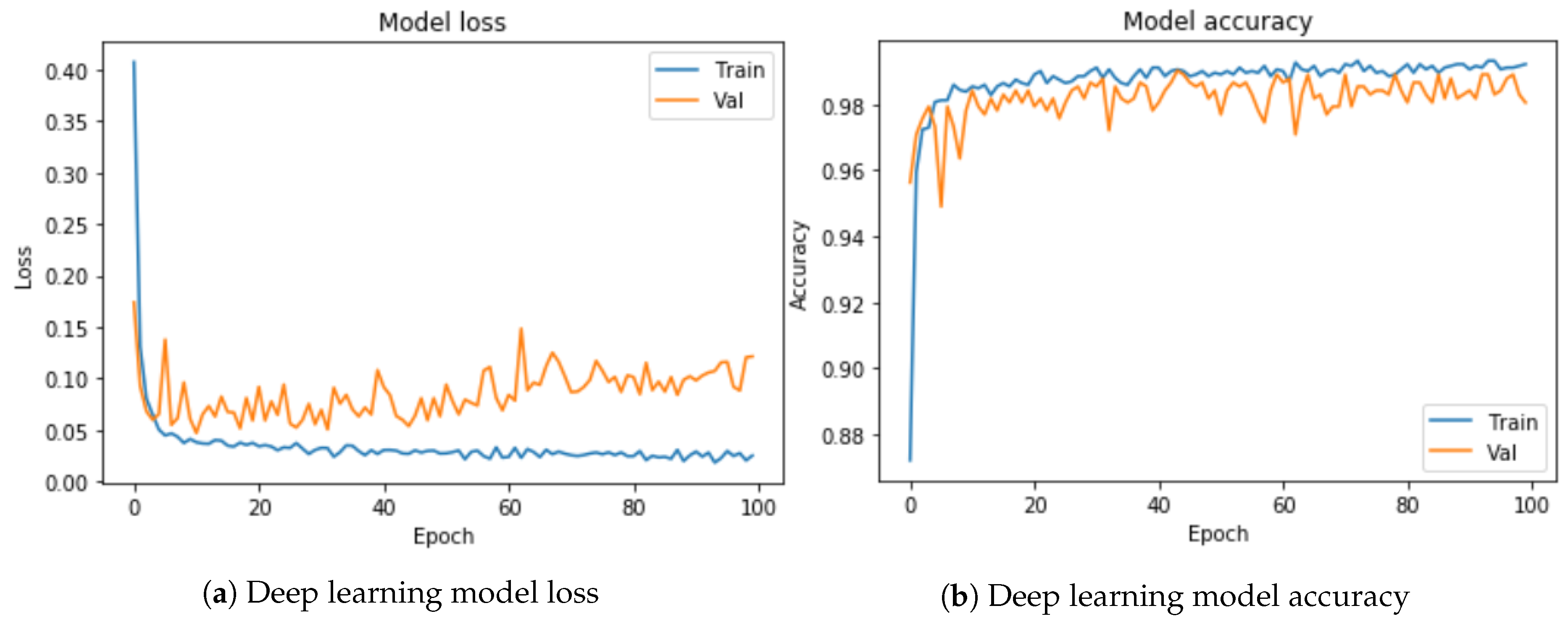The majority of the research that achieves state-of-the-art results usually uses a deep learning module with a ReLU activation function in the input and hidden layers [48]. For the output layer, we selected softmax as the activation function. The softmax activation function is used for building a multi-class classifier that solves the problem of assigning an instance to one class when the number of possible classes is more than two. Since in our experiment the number of independent variables is 10 and the number of prediction classes is 5, the number of neurons or units in the input and output layers are set to be 10 and 5 respectively. For each hidden layer 64 neurons are taken into consideration.

Figure 6 illustrates the deep learning model loss and accuracy. The classification results are given in Table 7.

4.3. Random Forest Classifier (RFC)

RFC [49,50] is the extended version of decision tree and it is a supervised ensemble classification algorithm. Several researchers including W. J. Al-Mudhafar [51] have used this classifier for electrofacies classification. This classifier builds a “forest” comprising numerous decision trees. In the random forest, each individual tree carries out a class prediction, and the class with the most votes becomes the model’s prediction.

Randomness is done in two stages. Firstly, bagging, a process of bootstrap aggregation, is used to modulate the training data that is available to each individual decision tree in the forest. Bagging is obtained for each tree, via random sampling with replacement. This duplicates some of the samples and will not select others. An average of approximately 63.2% of instances are used in each training subset, whereas the remaining approximately 37.8% “out-of-bag” samples are utilized for validation. The second form involves the selection of variables available to the classifier for splitting each node. At each node, a random subset of input variables selected from all available input variables and this is done by ranking them by their ability to produce a split threshold that maximizes the homogeneity of child nodes relative to the parent node. The decrease in the Gini index, as implemented by Breiman et al. (1984) and Breiman, (2001), provides this measure. The Gini index follows the following equation,

$$Gini\left(x\right)=\sum _{c=1}^l{h}_c(1-h_c)$$

(2)

where $h_c$ is the relative frequency of each class c, of a set comprising l classes, at a given node x; $h_c$ is given by

$$h_c=n_c/n,$$

(3)

where $n_c$ represents the amount of samples that comprise class c at any node and n represents the total samples that comprise that particular node.

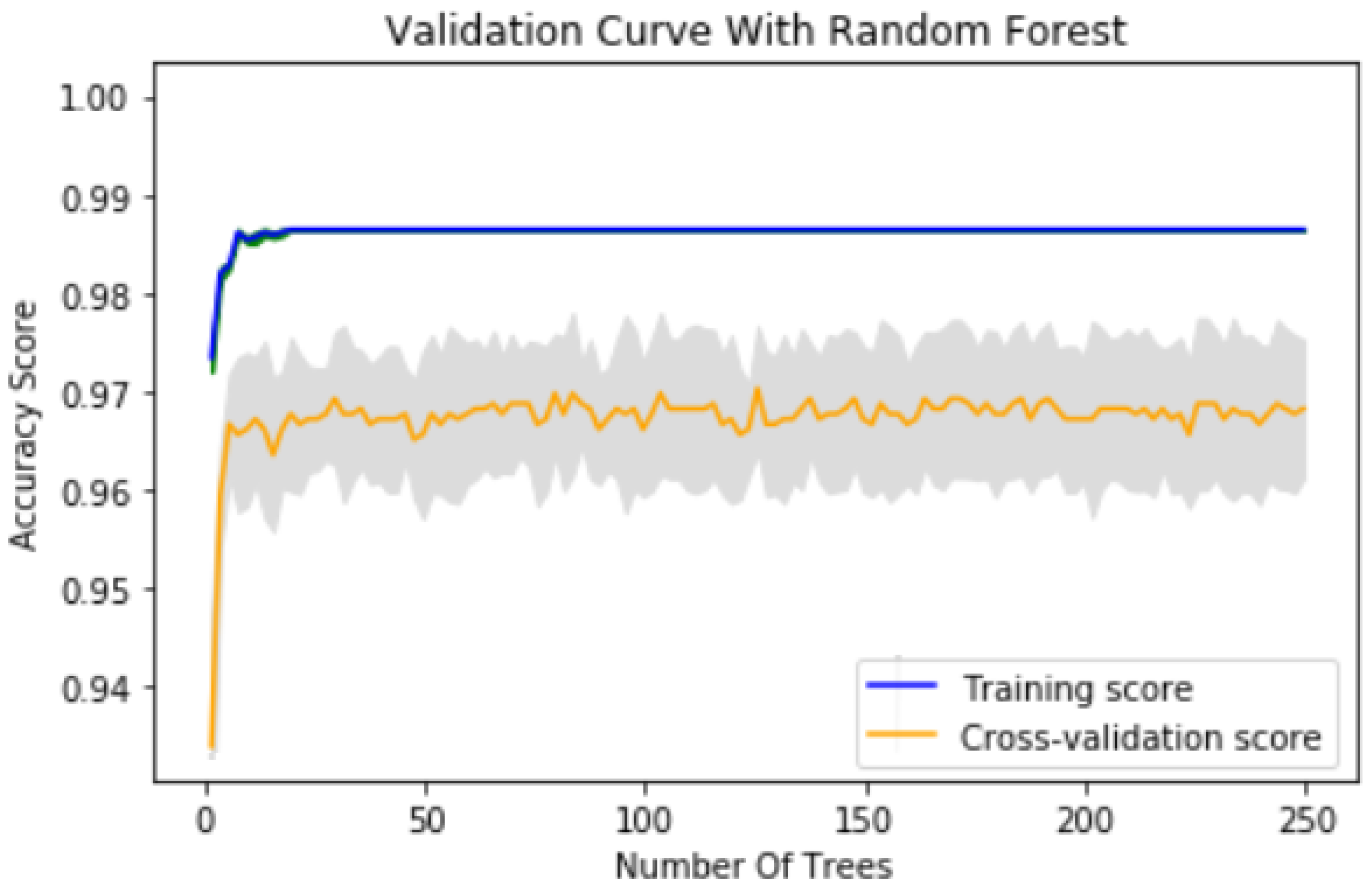
A total of 250 trees were considered in the RFC model which results the Training Accuracy of 0.986836 and the testing accuracy of 0.9706346.

In Table 7 the training and cross validation scores for lithology prediction are shown and Figure 7 illustrates the results.

4.4. Comparison Result

Table 7 below compares lithology prediction accuracy and percent difference (PD) among RST, SVM, deep learning and RFC.

5. Discussion and Conclusions

This research clarifies that the RST rule induction approach offers a unique and viable posterior classification approach to extract the patterns of how the electrofacies where constructed from the unique description of well log responses reflecting minerals and lithofacies from the logged interval by using the non-hierarchical k-means clustering algorithm. Electrofacies have a very significant bearing on reservoir parameter calculations like lithology, which is also shown in the experiment portion. RST provides efficient algorithms for finding hidden patterns in well log datasets and generates interpretable and understandable rules to classify the electrofacies with higher accuracy. The rules can explain the contributions of the well log attribute values in interpreting and classifying the electrofacies classes, which makes this module a unique whitebox electrofacies prediction module. It is also shown that, by analyzing the rules, valuable information on how the features contribute to interpreting the lithology classes can be extracted. A comparison study was also provided on the same datasets by employing some other renowned methods that have been used in this field, and we found that RST provides slightly better accuracy in classifying the electrofacies classes. Furthermore, RST provides a whitebox approach to classification, whereas deep learning, SVM or Random Forest provide only a blackbox prediction approach. However, despite RST being independent in its numerous achievements, to its tribute, in the future, for better accuracy, we will be working on multilayer RST to improve the prediction accuracy, by using larger datasets with more samples and datasets from several wells.

References

- Euzen, T.; Delamaide, E.; Feuchtwanger, T.; Kingsmith, K.D. Well Log Cluster Analysis: An Innovative Tool for Unconventional Exploration. In Proceedings of the CSUG/SPE 137822, Canadian Unconventional Resources and International Petroleum Conference, Calgary, AB, Canada, 19–21 October 2010. [Google Scholar]
- Tan, S.B.; Wang, Y.F.; Cheng, X.Q. Text feature ranking based on rough-set theory. In Proceedings of the IEEE/WIC/ACM International Conference on Web Intelligence, Fremont, CA, USA, 2–5 November 2007. [Google Scholar]
- Pawlak, Z. Rough Set Theory for Intelligent Industril Applications. In Proceedings of the Second International Conference on Intelligent Processing and Manufacturing of Materials. IPMM’99 (Cat. No.99EX296), Honolulu, HI, USA, 10–15 July 1999. [Google Scholar]
- Pawlak, Z. Rough sets. Int. J. Comput. Inf. Sci. 1982, 11, 341–356. [Google Scholar] [CrossRef]
- Busch, J.M.; Fortney, W.G.; Berry, L.N. Determination of lithology from well logs by statistical analysis. SPE Form Eval. 1987, 2, 412–418. [Google Scholar] [CrossRef]
- Sebtosheikh, M.A.; Motafakkerfard, R.; Riahi, M.A.; Moradi, S.; Sabety, N. Support vector machine method, a new technique for lithology prediction in an Iranian heterogeneous carbonate reservoir using petrophysical well logs. Carbonates Evaporites 2015, 30, 59–68. [Google Scholar] [CrossRef]
- Carrasquilla, A.; de Silvab, J.; Flexa, R. Associating fuzzy logic, neural networks and multivariable statistic methodologies in the automatic identification of oil reservoir lithologies through well logs. Rev. Geol. 2008, 21, 27–34. [Google Scholar]
- Lim, J.S.; Kang, J.M.; Kim, J. Interwell log correlation using artificial intelligence approach and multivariate statistical analysis. In SPE Asia Pacific Oil and Gas Conference and Exhibition; Society of Petroleum Engineers: Jakarta, Indonesia, 1999. [Google Scholar] [CrossRef]
- Chikhi, S.; Batouche, M. Hybrid neural network methods for lithology identification in the Algerian Sahara. World Acad. Sci. Eng. Tech. 2007, 4, 774–782. [Google Scholar]
- Chikhi, S.; Batouche, M. Using probabilistic unsupervised neural method for lithofacies identification. Int. Arab J. Inf. Technol. 2005, 2, 58–66. [Google Scholar]
- Cuddy, S.J. Litho-facies and permeability prediction from electrical logs using fuzzy logic. SPE Reserv. Eval. Eng. 2000, 3, 319–324. [Google Scholar] [CrossRef]
- Katz, S.A.; Vernik, L.; Chilingar, G.V. Prediction of porosity and lithology in siliciclastic sedimentary rock using cascade neural assemblies. J. Petrol. Sci. Eng. 1999, 22, 141–150. [Google Scholar] [CrossRef]
- Raeesi, M.; Moradzadeh, A.; Ardejani, F.D.; Rahimi, M. Classification and identification of hydrocarbon reservoir lithofacies and their heterogeneity using seismic attributes, logs data and artificial neural networks. J. Petrol. Sci. Eng. 2012, 82, 151–165. [Google Scholar] [CrossRef]
- Jacek, S.; Klaus, B.; Trond, R. Lithology classification from seismic tomography: Additional constraints from surface waves. J. Afr. Earth Sci. 2010, 58, 547–552. [Google Scholar]
- Gifford, C.M.; Agah, A. Collaborative multi-agent rock facies classification from wireline well log data. Eng. Appl. Artif. Intell 2010, 23, 1158–1172. [Google Scholar] [CrossRef]
- Priezzhev, I.; Stanislav, E. Application of machine learning algorithms using seismic data and well logs to predict reservoir properties. Presented at the 80th EAGE Conference Exhibition, Copenhagen, Denmark, 11–14 June 2018. [Google Scholar]
- Kim, Y.; Hardisty, R.; Torres, E.; Marfurt, K.J. Seismic-facies classfication using random forest algorithm. In SEG Technical Program Expanded Abstracts; Society of Exploration Geophysicists: Tulsa, OK, USA, 2018; pp. 2161–2165. [Google Scholar]
- Puskarczyk, E. Artificial neural networks as a tool for pattern recognition and electrofacies analysis in Polish palaeozoic shale gas formation. Acta Geophys. 2019, 67, 1991–2003. [Google Scholar] [CrossRef]
- Tang, H.; White, C.D. Multivariate statistical log log-facies classification on a shallow marine reservoir. J. Petrol. Sci. Eng. 2008, 61, 88–93. [Google Scholar] [CrossRef]
- Teh, W.J.; Willhite, G.P.; Doveton, J.H. Improved reservoir characterization in the ogallah field using petrophysical classifiers within electrofacies. In Proceedings of the SPE Improved Oil Recovery Symposium, Tulsa, OK, USA, 14–18 April 2012. [Google Scholar] [CrossRef]
- Schmitt, P.; Veronez, M.; Tognoli, F.; Todt, V.; Lopes, R.; Silva, C.; Lopes, R.C.; Silva, C.A.U. Electrofacies Modelling and Lithological Classification of Coals and Mud-bearing Fine-grained Siliciclastic Rocks Based on Neural Networks. Earth Sci. Res. 2013, 2. [Google Scholar] [CrossRef]
- Berteig, V.; Helgel, J.; Mohn, E.; Langel, T.; van der Wel, D. Lithofacies prediction from well data. In Proceedings of the Transactions of SPWLA 26th Logging Symposium Paper TT, Dallas, OK, USA, 17–20 June 1985; p. 25. [Google Scholar]
- Kiaei, H.; Sharghi, Y.; Ilkhchi, A.K.; Naderid, M. 3D modeling of reservoir electrofacies using integration clustering and geostatistic method in central field of Persian Gulf. J. Petrol. Sci. Eng. 2015, 135, 152–160. [Google Scholar] [CrossRef]
- Anxionnaz, H.; Delfiner, P.; Delhomme, J.P. Computer-generated corelike descriptions from open-hole logs. Am. Assoc. Petrol. Geol. 1990, 74, 375–393. [Google Scholar]
- Hernandez-Martinez, E.; Perez-Muñoz, T.; Velasco-Hernandez, J.X.; Altamira-Areyan, A.; Velasquillo-Martinez, L. Facies recognition using multifractal Hurst analysis: Applications to well-log data. Math. Geosci. 2013, 45, 471–486. [Google Scholar] [CrossRef]
- Euzen, T.; Power, M.R. Well log cluster analysis and electrofacies classification: A probabilistic approach for integrating log with mineralogical data. Am. Assoc. Petrol. Geol. Search Discov. 2014. Available online: http://www.searchanddiscovery.com/documents/2014/41277euzen/ndx_euzen.pdf (accessed on 21 March 2020).
- Kumar, B.; Kishore, M. Electrofacies classification—A critical approach. In Proceedings of the 6th International Conference and Exposition on Petroleum Geophysics, Kolkata, India, 8 January 2006; pp. 822–825. [Google Scholar]
- Tang, H. Successful Carbonate Well Log Facies Prediction Using an Artificial Neural Network Method: Wafra Maastrichtian Reservoir, Partitioned Neutral Zone (PNZ). Saudi Arabia and Kuwait. In Proceedings of the SPE Annual Technical Conference and Exhibition, New Orleans, LA, USA, 4–7 October 2009. [Google Scholar]
- Deng, C.; Pan, H.; Fang, S.; Konaté, A.A.; Qin, R. Support vector machine as an alternative method for lithology classification of crystalline rocks. J. Geophys. Eng. 2017, 14, 341–349. [Google Scholar] [CrossRef]
- Hossain, T.M.; Watada, J.; Hermana, M.; Sakai, H. A rough set based rule induction approach to geoscience data. In Proceedings of the International Conference of Unconventional Modelling, Simulation & Optimization on Soft Computing and Meta Heuristics, UMSO 2018, Fukuok, Japan, 2–5 December 2018; Available online: https://ieeexplore.ieee.org/document/8637237 (accessed on 21 May 2019).
- Hossain, T.M.; Watada, J.; Hermana, M.; Aziz, I.A.A. Supervised Machine Learning in Electrofacies Classification: A Rough Set Theory Approach. In Proceedings of the ICISE 2020, Kota Bharu, Malaysia, 29–30 January 2020. [Google Scholar]
- Hossain, T.M.; Watada, J.; Jian, Z.J.; Sakai, H.; Rahman, S.A.; Aziz, I.A.A. Machine Learning Based Missing Data Imputation: An NIS Apriori Approach to Predict Complex Lithology. IJICIC 2020, 16, 1077–1091. [Google Scholar]
- Geurts, P.; Ernst, D.; Wehenkel, L. Extremely randomized trees. Mach. Learn. 2006, 36, 3–42. [Google Scholar]
- Raileanu, L.E.; Stoffel, K. Theoretical Comparison between the Gini Index and Information Gain Criteria. Ann. Math. Artif. Intell. 2004, 41, 77–93. [Google Scholar] [CrossRef]
- Louppe, G.; Wehenkel, L.; Sutera, A.; Geurts, P. Understanding variable importances in forests of randomized trees. In Advances in Neural Information Processing Systems; Burges, C.J.C., Bottou, L., Welling, M., Ghahramani, Z., Weinberger, K.Q., Eds.; Curran Associates Inc.: New York, NY, USA, 2013; pp. 431–439. [Google Scholar]
- Menze, B.H.; Kelm, B.M.; Masuch, R.; Himmelreich, U.; Bachert, P.; Petrich, W.; Hamprecht, F.A. A comparison of random forest and its Gini importance with standard chemometric methods for the feature selection and classification of spectral data. BMC Bioinform. 2009, 10, 213. [Google Scholar] [CrossRef] [PubMed]
- Nashawi, I.S.; Malallah, A. Improved Electrofacies Characterization and Permeability Predictions in Sandstone Reservoirs Using a Data Mining and Expert System Approach. Petrophysics 2009, 50, 250–268. [Google Scholar]
- Lim, J.-S.; Kang, J.M.; Kim, J. Multivariate Statistical Analysis for Automatic Electrofacies Determination from Well Log Measurements. Presented at the 1997 SPE Asia Pacific Oil and Gas Conference, Kuala Lumpur, Malaysia, 14–16 April 1997. [Google Scholar]
- Li, H.; Yang, X.; Wei, W.H. The Application of Pattern Recognition in Electrofacies Analysis. Intell. Model. Verif. 2014, 2014, 640406. [Google Scholar] [CrossRef]
- Kanungo, T.; Mount, D.M.; Netanyahu, N.S.; Piatko, C.D.; Silverman, R.; Wu, A.Y. An efficient k-means clustering algorithm: Analysis and implementation. IEEE Trans Pattern Anal. Mach. Intell. 2002, 24, 881–892. [Google Scholar] [CrossRef]
- Lazhari, T. Electrofacies classification using Principal Component Analysis PCA and Multi Layer Perception MLP, Triassic fluvial Lower Serie reservoir. Oued Mya Basin. Algeria. 2018. [Google Scholar] [CrossRef]
- Nguyen, S.H. On Efficient Handling of Continuous Attributes in Large Data Bases. Fundam. Inform. 2001, 48, 61–81. [Google Scholar]
- Evgeniou, T.; Pontil, M. Support Vector Machines: Theory and Applications. Machine Learning and Its Applications; Georgios, P., Vangelis, K., Constantine, D.S., Eds.; Springer: Berlin/Heidelberg, Germany, 2001; Volume 2049, pp. 249–257. [Google Scholar]
- Alexsandro, G.C.; Carlos, A.D.P.; Geraldo, G.N. Facies classification in well logs of the Namorado oil field using Support Vector Machine algorithm. In Proceedings of the 15th International Congress of the Brazilian Geophysical Society & EXPOGEF, Rio de Janeiro, Brazil, 31 July–3 August 2017. [Google Scholar] [CrossRef]
- Li, G.H.; Qiao, Y.H.; Zheng, Y.F.; Li, Y.; Wu, W.J. Semi-Supervised Learning Based on Generative Adversarial Network and Its Applied to Lithology Recognition. IEEE Access 2019, 7, 67428–67437. [Google Scholar] [CrossRef]
- Imamverdiyev, Y.; Sukhostat, L. Lithological facies classification using deep convolutional neural network. J. Pet. Sci. Eng. 2019, 174, 216–228. [Google Scholar] [CrossRef]
- Karpathy, A. A Peek at Trends in Machine Learning. 8 April 2017. Available online: https://medium.com/karpathy/a-peek-at-trends-in-machine-learning-ab8a1085a106 (accessed on 5 July 2020).
- Brownlee, J. A Gentle Introduction to the Rectified Linear Unit (ReLU) in Deep Learning Performance. 9 January 2019. Available online: https://machinelearningmastery.com/rectified-linear-activation-function-for-deep-learning-neural-networks/ (accessed on 5 July 2020).
- Breiman, L. Random forests. Mach. Learn. 2001, 45, 5–32. [Google Scholar] [CrossRef]
- Shah, S.H.; Angel, Y.; Houborg, R.; Ali, S.; McCabe, M.F. A Random Forest Machine Learning Approach for the Retrieval of Leaf Chlorophyll Content in Wheat. Remote Sens. 2019, 11, 920. [Google Scholar] [CrossRef]
- Al-Mudhafar, W.J. Advanced Supervised Machine Learning Algorithms for Efficient Electrofacies Classification of A Carbonate Reservoir in A Giant Southern Iraqi Oil Field. In Proceedings of the Offshore Technology Conference, Houston, TX, USA, 4–7 May 2020. [Google Scholar] [CrossRef]
© 2020 by the authors. Licensee MDPI, Basel, Switzerland. This article is an open access article distributed under the terms and conditions of the Creative Commons Attribution (CC BY) license (http://creativecommons.org/licenses/by/4.0/).