Training and Testing of a Single-Layer LSTM Network for Near-Future Solar Forecasting

Abstract

Increasing integration of renewable energy sources, like solar photovoltaic (PV), necessitates the development of power forecasting tools to predict power fluctuations caused by weather. With trustworthy and accurate solar power forecasting models, grid operators could easily determine when other dispatchable sources of backup power may be needed to account for fluctuations in PV power plants. Additionally, PV customers and designers would feel secure knowing how much energy to expect from their PV systems on an hourly, daily, monthly, or yearly basis. The PROGNOSIS project, based at the Cyprus University of Technology, is developing a tool for intra-hour solar irradiance forecasting. This article presents the design, training, and testing of a single-layer long-short-term-memory (LSTM) artificial neural network for intra-hour power forecasting of a single PV system in Cyprus. Four years of PV data were used for training and testing the model (80% for training and 20% for testing). With a normalized root mean squared error (nRMSE) of 10.7%, the single-layer network performed similarly to a more complex 5-layer LSTM network trained and tested using the same data. Overall, these results suggest that simple LSTM networks can be just as effective as more complicated ones.

1. Introduction

Many countries around the world have been transitioning from fossil fuels to more renewable energy sources to mitigate the effects of climate change. Because the current energy grid is built around dispatchable sources of power, the intermittency and variance of many renewable energy sources, such as solar and wind, makes large-scale integration difficult. To meet this challenge, new tools must be developed to aid grid operators and energy utilities in accurately predicting the output of renewable power plants on an hourly or daily basis. Accurate intra-hour forecasts would alert grid operators to when other backup sources of power should be brought online or ramped down. With reliable day-ahead energy forecasts, the sale and purchase of prospective power across the boarders of independent system operators (ISOs) would become easier. One of the goals of the PROGNOSIS project, a research project based at the Cyprus University of Technology, is to develop a “dynamic data assimilation model for intra-hour forecasting of solar irradiance over a specific area taking into consideration the presence of clouds/aerosols over the area” [1].

One PROGNOSIS sub-project is to research the use of artificial neural networks (ANNs) as a method for near-future solar forecasting. While many ANN models for solar forecasting have been developed over the past several years, few use solely endogenous data. Rather, they rely on meteorological data which can be expensive to obtain. This article presents the training, testing, and performance of a single-layer long-short-term memory (LSTM) network for intra-hour solar forecasting of a single PV system in Cyprus. The performance of the single-layer LSTM network is compared to a previously-developed 5-layer LSTM network trained using the same data.

1.1. Background

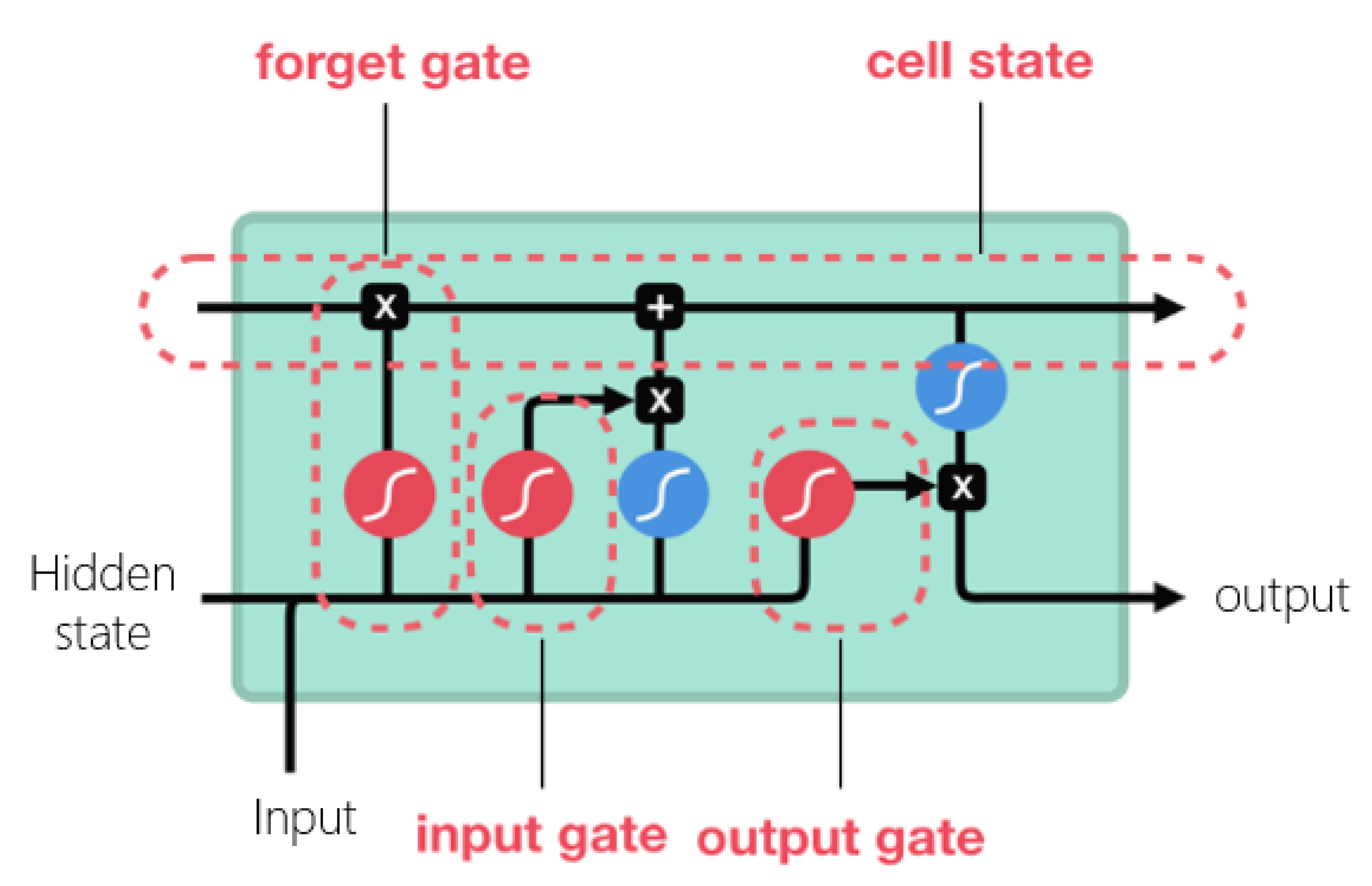
1.1.1. Theory of LSTM Networks

Machine learning has gained popularity over the past several years, and engineers have developed many different types of machine learning models. Two of the more popular models for prediction and forecasting, are support-vector machines (SVMs) and artificial neural networks (ANNs). In recent years, a significant body of research has been published on the application of ANNs for solar forecasting.

As James Dacombe defines in his article An Introduction to Artificial Neural Networks, “An Artificial Neural Network is an information processing model that is inspired by the way biological nervous systems, such as the brain, process information. They are loosely modeled after the neuronal structure of the mammalian cerebral cortex but on much smaller scales” [2]. Neurons, the most basic components of an ANN take two or more inputs and give one output. They then compute an output based on a set of weights (applied to the inputs) and a bias (which modifies the output). When several neurons are organized into layers and connected such that the output of one layer feeds into the input of another layer, this creates a feedforward ANN that can learn to solve complex problems using the experience it gained during the training process [2].

ANNs learn by example. During the training process, an ANN is given a set of inputs to process. The output from the ANN is then compared to the desired output, and an error is calculated. After a set of training examples has been processed, a backpropagation algorithm tweaks the weights and biases using gradient descent to reduce the error. This process is repeated many times until the error function converges, or the researcher is satisfied with the ANN’s performance. Once effectively trained, an ANN can be fed new data and predict the correct output with relatively high precision.

Recurrent neural networks (RNNs) are popular for predicting time series data. For each timestep, the RNN receives not only the new input data but also its own output from the previous timestep, known as the hidden state. In this way, RNNs have a rudimentary form of short-term memory and are better at finding short-term trends in the data than plain feedforward networks [3].

LSTM networks are a type of RNN. The LSTM modules are typically referred to as cells rather than neurons and contain a series of gates. A diagram of an LSTM cell can be seen in Figure 1. Each LSTM cell has a form of longer-term memory in the form of a cell state that is updated through time. A forget gate looks at the new input and the hidden state and decides which information in the cell state can be safely forgotten. The input gate then decides what information from the new input should be added to the cell state to be remembered. Finally, the output gate takes information from the cell state, input, and hidden state and generates the output for the current time step. In this way, LSTM networks can remember information through many timesteps, making them ideal for finding longer-term trends in data. At the same time, the LSTM cell still uses the hidden state, and therefore has short-term memory as well. Overall, LSTM networks can be a powerful tool in time series forecasting [4,5].

ANNs perform best when the training data adheres to certain conditions. First, when all the data have been cleaned and processed so that there are no wrong, not-a-number values or significant time gaps in the data. Secondly, because ANNs have no concept of units but rather look only at the numerical value of the input, it is advisable to normalize all training inputs to be within the same range. Feature scaling prevents the ANN from learning false patterns that result from unit differences in the data. A common practice is to use feature scaling to map all the data to between 0 and 1. Feature scaling the inputs has the additional effect of speeding up the training process of the ANN because small changes in the weights and biases will have a greater and more consistent effect on the output [6].

ANNs have several hyperparameters that can be tweaked and customized to particular applications. These hyperparameters include the number of hidden layers, the number of neurons per layer, batch size, and the number of training epochs. When designing an ANN, multiple experiments are needed to find the optimal hyperparameters for the specific application. There are a few heuristic guides that ANN designers can use to optimize their hyperparameters. According to one of the most common heuristics, each layer of the ANN adds a level of abstraction to the prediction or classification function. Each neuron in the first layer linearly approximates a section of the input. The additional layers would combine these pieces into a more continuous function and the next could add curvature or an offset to the prediction function [7].

That being said, the best way to optimize an ANN is with simple trial and error. Each problem is going to be unique, and, heuristics aside, even a single-layer ANN can provide a reasonable amount of abstraction with enough neurons. There are a few signs that researchers look for to indicate if their network is to large or too small for their application. Networks that are too small, generally will not perform well because they do not have enough parameters (weights and biases) to properly fit to the data. If a network is too large, it will be slow to train and can overfit the data. Overfitting is when a model learns the particular patterns of the training data too well, making it difficult to extrapolate to new data. An overfit model can have high accuracy when used to predict the training data, but poor performance when given new data to predict [7].

1.1.2. Related Studies from Literature

Over the past several years, there has been increasing interest and investigation into using LSTM networks for solar forecasting. Many of these methods, such as those presented in [8], require exogenous meteorological data.

In [8], Donghun Lee et al. developed two LSTM models for hourly PV power forecasting in Gumi City, South Korea. Their first LSTM model received six inputs: temperature, humidity, cloudiness, radiation, month, and day. Their second LSTM model used only the four meteorological inputs and omitted the seasonal information of month and day. Both models had three hidden layers and gave a single output of PV power for the next hour. The seasonal LSTM model outperformed all the other forecast models it was compared to including an ARIMA, seasonal ARIMA, simple feedforward ANN, deep-learning ANN, and a seasonal deep-learning ANN.

In [9], Abdel-Nasser et al. developed several LSTM models for 1-hour ahead solar power forecasting in Aswan and Cario Egypt. They trained and tested five different LSTM architectures with varying inputs, numbers of layers, and type of LSTM. All of their models used purely endogenous, historical PV data as input. Their base LSTM model (Model 1) received the PV production value as its only input one hour prior to the desired forecast time. It had a single hidden layer which consisted of four LSTM cells. Their second model (Model 2) was similar to Model 1 except it received production values from the last three, one-hour timesteps as separate input features to forecast one-hour ahead. Their third model (Model 3) processed the last three timesteps through a single input feature before calculating its forecasted value. Model 4 is similar to Model 1 except that it used stateful LSTM blocks which enabled the network to remember trends across training batches. Finally, their Model 5 was a two-layer, stateful LSTM network.

The researchers in [9] used 70% of their data for training and 30% for testing. Each model was evaluated after being trained with 20, 50 and 100 epochs. Model 3, trained with 50 epochs performed the best. The researchers compared Model 3’s performance to a multiple-linear regression model (MLR), a bagged regression trees (BRT) model, and a simple feedforward neural network model, all of which were trained using the same data. Nasser et al. found that the Model 3 LSTM network significantly outperformed the MLR, BRT and feedforward neural network.

While LSTM models using meteorological data show promise, depending on the location of the PV system being forecasted, exogenous data like those used in [8] may be unavailable, expensive to obtain or unreliable. Because of these potential problems, the PROGNOSIS project aims to develop LSTM models that use only endogenous, historical PV production data as their input.

Our study is similar to [9] in that it explores different LSTM architectures for solar forecasting using only endogenous data. Two main differences exist between our study and [9]. The most significant difference is that our study uses 192, 15-min timesteps as input instead of the 1-2, one-hour timesteps used in [9]. Our larger number of timesteps can take better advantage of the LSTM cell’s ability to remember longer-term trends in the data. The 15 min sample time provided our forecast models with greater temporal resolution which could be more helpful to grid operators than an hourly forecast. Additionally, Ref. [9] used relatively small LSTM networks of one or two layers with four LSTM cells per layer, whereas our study investigates one and five layer LSTM networks with 50 LSTM cells per layer. As LSTM optimization is largely trial and error, it was possible that our, the slightly larger networks would perform better than the smaller ones presented in [9].

2. Data and Methods

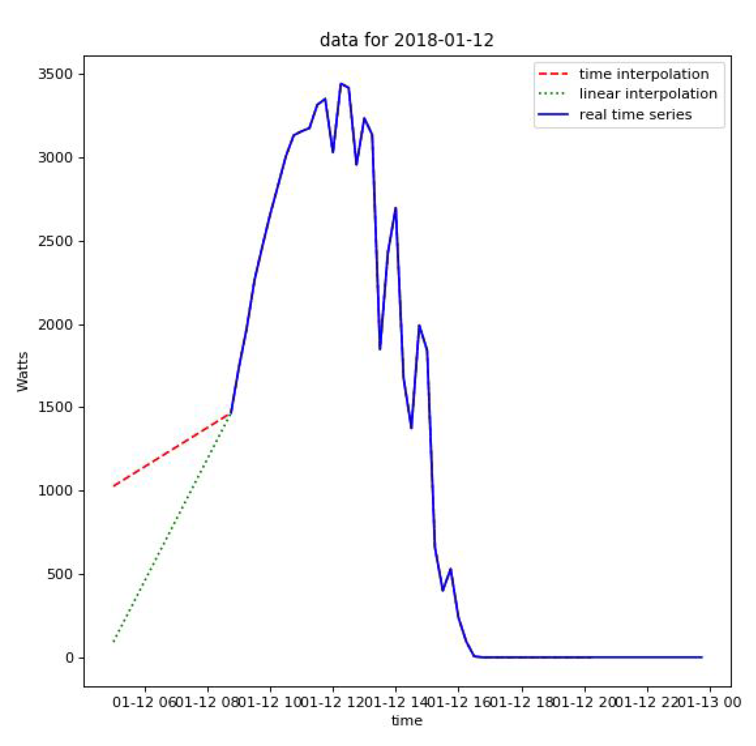
2.1. Data Preprocessing Methods

Before training or testing an ANN, the training and testing data must go through a series of preprocessing steps. These methods included removing any unnecessary information, interpolating any missing data points, and organizing the energy production data chronologically. Finally, the resulting data column was normalized using feature scaling before it was used as input to the LSTM network.

All data preprocessing was done in Python 3.6 using the Spyder integrated development environment (IDE) through Anaconda. The Python script contained all the functions that were used to process the Cyprus PV data and build, train, and validate the single-layer LSTM network.

The first step in data preprocessing was to load the data into Python and reformat it. The original data files were separated by month, and each column represented a day of PV generated DC energy. Once reformatted, all the data were loaded into a single data frame with a DateTime index.

Once the data were formatted, the quality of the data was evaluated. A function was developed to search for and record the location of any nan, negative, and duplicate values. To reduce the number of zeros in the data frame, the nighttime values between 20:00 h and 5:15 h were removed. The times were specifically chosen so that the LSTM network trained on these data could be directly compared to the existing, previously trained LSTM network. After removing the nighttime data, the missing data were interpolated, using the time or linear interpolation method.

2.2. Data Quality and Preprocessing

The Cyprus PV data contained energy production data from a single PV system over four years of study (2016–2019). The data had a sample rate of 15 min and contained energy production values ranging from 0 to 5 kW. There were no significant time gaps in the time series. The PV production data had 90 nan values, all of which occurred in 2017 and 2018, accounting for 0.1062% of the data. There were no negative or duplicate data entries. As stated in the Methods section, all the data between 20:00 h and 5:15 h were removed to reduce the number of zeros in the final data frame.

Two interpolation methods were considered to fill in the nan values: time interpolation and linear interpolation, both of which are built-in methods of the Pandas Python library’s interpolation function. The time interpolation method was specially designed for time series data, while linear interpolation uses a linear function. To determine which interpolation method was best, several days from the Cyprus data were chosen and the missing entries were interpolated using both methods. The results were then visually compared. Although in most cases, the time and linear methods generated very similar results, there were a couple of days where they differed significantly. Figure 2 shows one such day.

In this instance, linear interpolation outperformed the time interpolation, reaching 0 at the beginning of the day as it should. However, this example was not sufficient to definitively determine if linear interpolation outperformed time interpolation. It was decided to train two identical neural networks, one that used time-interpolated data and one that used linearly interpolated data. The performances of these two networks were then compared to determine which model was more accurate. The results of this comparison are in Section 3.

2.3. LSTM Building, Training, and Evaluation

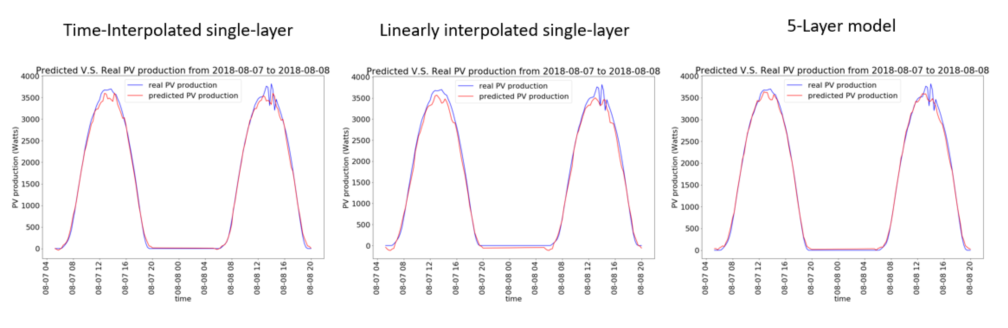
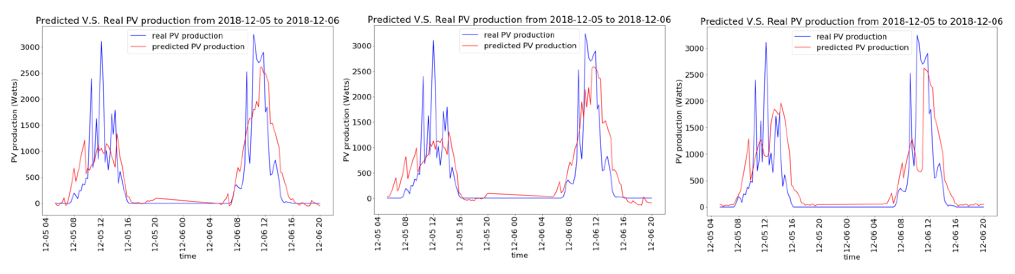
Before the data were used to train the LSTM network, they were split into a training set and a test set. The data were split by assigning the first 80% to the training set and the last 20% to the testing set. Next, the DateTime columns were removed from the training and test sets, leaving a single column of energy production data in each set. Those columns were then normalized to between zero and one using feature scaling. Finally, the training and testing sets were split into input and target arrays. Each row of the input arrays contained a vector of length 192 and represented the input for a single training example. Each row of the target arrays contained a vector of length 6 and represented the 6 target values for a single training example. Each of the 6 target values were the next 6 energy production values directly following the corresponding input vector of 192 values. The time window of inputs and outputs then shifted by 6 values so that the first value in a given input vector is the same as the 7th value in the previous input vector. This way, the outputs and targets do not overlap, but rather are continuous in time.

To illustrate the building of the input and target vectors consider the following theoretical PV data column: [A1, A2, A3, …, An]. The first input vector would be [A1, A2, A3, …, A192] and the corresponding first target vector would be [A193, A194, A195, A196, A197, A198]. The second input vector would be [A7, A8, …, A198] and the second target vector would be [A199, A200, A201, A202, A203, A204].

The Keras Python library was used to build, train and test the LSTM network. The LSTM model was built upon Keras’s sequential class. A single hidden layer of 50 neurons and an output layer of 6 neurons were added. The "Adam" optimizer was chosen for training. Once built, the LSTM was trained and tested using the training and test sets, respectively. The model underwent 100 epochs of training with a batch size of 32, dropout rate of 0.2, and the "Adam" optimizer function. In addition to the test results, a 10-fold cross-validation process was used to evaluate the model.

This entire building, training and testing process was conducted twice, once with the time-interpolated data sets and once with the linearly interpolated data sets.

3. Results

The single-layer LSTM network received 192 timesteps of the PV system’s energy production data and forecasted 6 timesteps into the future. Each timestep was 15 min, so the model received just over three days of data as input and forecasted up to 1.5 h into the future. Both the single-layer models and the 5-layer model to which they were compared had 50 neurons in each hidden layer.

Table 1. Test results for single-layer and 5-layer LSTM model.

	RMSE (W)	nRMSE	MBE (W)	MAE (W)	${\mathit{R}}^2$
time-interpolated single-layer model	450.90	10.7%	26.56	235.10	0.882
linearly interpolated single-layer model	455.35	10.8%	1.30	259.39	0.879
5-layer (time interpolated) model	478.25	11.4%	76.2	240.65	0.868

shows results from testing the two single-layer LSTM models with the test sets and compares their performances with that of the pre-existing 5-layer LSTM network. The RMSE is the standard deviation of the residuals and is a measure of how well a regression fits a set of data [10]. The nRMSE is the RMSE divided by the mean of the data [11], which makes it possible to compare the results between models regardless of units. The MBE is a measure of the average bias in the prediction and indicates whether the model tends to over or under estimate [12]. The MAE measures the average error between the forecasted and actual values [13]. The $R^2$ value measures the strength of the relationship between the forecasted and actual values where 1 represents a strong correlation and 0 represents no correlation. In addition to the test data, 10-fold validation was used to evaluate the model. The results of the validation are shown in

Table 2. The 10-fold validation results for single-layer LSTM models.

	Mean Squared Error (W)${}^2$	Variance (W)
time-interpolated single-layer model	0.0097	0.0069
linearly interpolated single-layer model	0.0010	0.0075

in the form of the mean squared error (MSE) and variance.

To further explore how well the three models forecasted under different conditions, Figure 3 shows how they performed under sunny conditions and Figure 4 shows how they performed under cloudy conditions. As expected, the forecasts follow the trends in the sunny day data very well. The cloudy day forecasts, though less accurate, do a commendable job of capturing some of the fluctuations in PV production when clouds pass over.

It is clear from Table 1, and Figure 3 and Figure 4 that the two single-layer models perform very similarly to the five-layer model across most of the performance metrics. The notable exception is the MBE of the linearly interpolated, single-layer model which seems abnormally low.

The fact that the performance of a large five-layer LSTM network could be replicated so closely by two, much smaller networks suggests that five layers may be overly complicated for this application.

4. Discussion and Conclusions

Although many studies use ANNs for solar forecasting, few employ LSTM networks specifically. The majority of the research to date uses deep-learning multi-layer perceptron networks or RNNs. During our literature review of over 30 research papers, it was found that these ANN and RNN models achieved nRMSE values of around 10–30% with the occasional outlier performing better or worse. According to [14], the average nRMSE for published machine learning solar forecasting models in 2018 was 23% with a low mean bias error and relatively high volatility. More than anything else, the accuracy of ANN models depend on location and weather predictability. The models that had lower nRMSE values tended to be in locations such as Greece [15], Corsica island [16] and Senegal [17] where the weather is consistently sunny for a significant portion of the year.

At 10.7% and 10.8% nRMSE, the error of the single-layer models presented in this article fall at the low end of the published spectrum. Given the predictability of Cyprus weather, this is not surprising. What this study does show, however, is that LSTM networks are at least as good as the other, more well-researched ANNs for near-future solar forecasting. Additionally, because the single-layer LSTM networks performed similarly to the five-layer LSTM network, smaller LSTM networks may be able to accomplish quite complicated tasks as well as, or better than their larger counterparts. Most of the high-performing ANN models use large multi-layered networks that are slow to train and require high processing power. If a single-layer LSTM network can achieve the same results as a larger MLP, or a larger LSTM, it would be more economical to choose the smaller LSTM network.

Of course, this is a small-scale study, and further research would have to be done to confirm these findings. Specifically the performance of single-layer LSTM networks should be compared to that of larger LSTM and deep-learning MLP networks in several differing climates to see if they are indeed superior for solar forecasting.

References

1. “PROGNOSIS”, Sustainable Energy Laboratory. Available online: https://www.energylab.ac.cy/projects/prognosis/en/ (accessed on 21 June 2020).
2. Dacombe, J. An Introduction to Artificial Neural Networks (with Example); Medium: San Francisco, CA, USA, 2017; Available online: https://medium.com/@jamesdacombe/an-introduction-to-artificial-neural-networks-with-example-ad459bb6941b (accessed on 21 June 2020).
3. A Beginner’s Guide to LSTMs and Recurrent Neural Networks. Pathmind. Available online: http://pathmind.com/wiki/lstm (accessed on 13 December 2019).
4. Nguyen, M. Illustrated Guide to LSTM’s and GRU’s: A Step by Step Explanation; Medium: San Francisco, CA, USA, 2019; Available online: https://towardsdatascience.com/illustrated-guide-to-lstms-and-gru-sa-step-by-step-explanation-44e9eb85bf21 (accessed on 13 December 2019).
5. Zaouali, K.; Rekik, R.; Bouallegue, R. Deep Learning Forecasting Based on Auto-LSTM Model for Home Solar Power Systems. In Proceedings of the 2018 IEEE 20th International Conference on High Performance Computing and Communications; IEEE 16th International Conference on Smart City; IEEE 4th International Conference on Data Science and Systems (HPCC/SmartCity/DSS), Exeter, UK, 28–30 June 2018; pp. 235–242. [Google Scholar] [CrossRef]
6. Brownlee, J. How to Use Data Scaling Improve Deep Learning Model Stability and Performance; Machine Learning Mastery: Vermont, Australia, 2019; Available online: https://machinelearningmastery.com/howto-improve-neural-network-stability-and-modeling-performance-with-data-scaling/ (accessed on 22 June 2020).
7. Brownlee, J. How to Configure the Number of Layers and Nodes in a Neural Network; Machine Learning Mastery: Vermont, Australia, 2018; Available online: https://machinelearningmastery.com/how-to-configure-the-number-of-layers-and-nodes-in-a-neural-network/ (accessed on 23 June 2020).
8. Lee, D.; Kim, K. Recurrent Neural Network-Based Hourly Prediction of Photovoltaic Power Output Using Meteorological Information. Energies 2019, 12, 215. [Google Scholar] [CrossRef] [Green Version]
9. Abdel-Nasser, M.; Mahmoud, K. Accurate photovoltaic power forecasting models using deep LSTM-RNN. Neural Comput. Appl. 2017. [Google Scholar] [CrossRef]
10. RMSE: Root Mean Square Error—Statistics How To. Available online: https://www.statisticshowto.datasciencecentral.com/rmse/ (accessed on 13 December 2019).
11. rrmse: Relative Root Mean Square Error in Fgmutils: Forest Growth Model Utilities. Available online: https://rdrr.io/cran/Fgmutils/man/rrmse.html (accessed on 13 December 2019).
12. Mean Bias Error—An overview | ScienceDirect Topics. Available online: https://www.sciencedirect.com/topics/engineering/mean-bias-error (accessed on 13 July 2020).
13. Stephanie. Absolute Error & Mean Absolute Error (MAE). Statistics How to. 25 October 2016. Available online: https://www.statisticshowto.com/absolute-error/ (accessed on 13 July 2020).
14. Blaga, R.; Sabadus, A.; Stefu, N.; Dughir, C.; Paulescu, M.; Badescu, V. A current perspective on the accuracy of incoming solar energy forecasting. Prog. Energy Combust. Sci. 2019, 70, 119–144. [Google Scholar] [CrossRef]
15. Kardakos, E.G.; Alexiadis, M.C.; Vagropoulos, S.I.; Simoglou, C.K.; Biskas, P.N.; Bakirtzis, A.G. Application of time series and artificial neural network models in short-term forecasting of PV power generation. In Proceedings of the 2013 48th International Universities’ Power Engineering Conference (UPEC), Dublin, Ireland, 2–5 September 2013; pp. 1–6. [Google Scholar] [CrossRef]
16. Paoli, C.; Voyant, C.; Muselli, M.; Nivet, M.-L. Forecasting of preprocessed daily solar radiation time series using neural networks. Sol. Energy 2010, 84, 2146–2160. [Google Scholar] [CrossRef] [Green Version]
17. Nkounga, W.M.; Ndiaye, M.F.; Ndiaye, M.L.; Cisse, O.; Bop, M.; Sioutas, A. Short-term forecasting for solar irradiation based on the multi-layer neural network with the Levenberg-Marquardt algorithm and meteorological data: Application to the Gandon site in Senegal. In Proceedings of the 2018 7th International Conference on Renewable Energy Research and Applications (ICRERA), Paris, France, 14–17 October 2018; pp. 869–874. [Google Scholar] [CrossRef]
Figure 1. Diagram of an LSTM cell [3].
Applsci 10 05873 g001
Figure 2. Linear vs. time interpolation methods on a single, incomplete day of PV data.
Applsci 10 05873 g002
Figure 3. Examples of real vs. forecasted PV production for sunny days.
Applsci 10 05873 g003
Figure 4. Examples of real vs. forecasted PV production for cloudy days.
Applsci 10 05873 g004