Abstract
Photovoltaic (PV) monitoring and fault detection are very crucial to enhance the service life and reliability of PV systems. It is difficult to detect and classify the faults at the Direct Current (DC) side of PV arrays by common protection devices, especially Line-to-Line (LL) faults, because such faults are not detectable under high impedance fault and low mismatch conditions. If these faults are not diagnosed, they may significantly reduce the output power of PV systems and even cause fire catastrophe. Recently, many efforts have been devoted to detecting and classifying LL faults. However, these methods could not efficiently detect and classify the LL faults under high impedance and low mismatch. This paper proposes a novel fault diagnostic scheme in accordance with the two main stages. First, the key features are extracted via analyzing Current–Voltage (I–V) characteristics under various LL fault events and normal operation. Second, a genetic algorithm (GA) is used for parameter optimization of the kernel functions used in the Support Vector Machine (SVM) classifier and feature selection in order to obtain higher performance in diagnosing the faults in PV systems. In contrast to previous studies, this method requires only a small dataset for the learning process and it has a higher accuracy in detecting and classifying the LL fault events under high impedance and low mismatch levels. The simulation results verify the validity and effectiveness of the proposed method in detecting and classifying of LL faults in PV arrays even under complex conditions. The proposed method detects and classifies the LL faults under any condition with an average accuracy of 96% and 97.5%, respectively.
1. Introduction
With the increasing global growth of photovoltaic (PV) installations, autonomous monitoring of PV systems has become increasingly important to diagnose system and component failures as fast as possible in order to ensure the long-term reliability and service life of PV systems [1,2,3]. PV arrays may fail due to internal and the external causes. The line-to-line (LL) fault is one of the major catastrophic failures that can lead to lower system efficiency and even worse, to fire disaster. An LL fault is defined as an unintentional connection between two points in a PV array with a different potentials [4,5]. LL faults might occur in PV arrays due to mechanical damage, water ingress, DC junction box corrosion, and hot spots caused by the back-sheet failures.
For a better understanding of LL faults, Figure 1 shows the most common configuration of a PV array, which includes the PV arrays affected by two types of LL faults, and the conventional protection devices such as Over Current Protection Devices (OCPD), namely fuses. Here, the intensity of an LL fault is expressed by the level of the mismatch, which is specified by the number of modules affected by LL faults. As shown in Figure 1, F1 represents a LL fault with 10% mismatch due to the short-circuit that occurs between the external contacts, i.e., the incoming and outgoing connection of a single PV module in a string. Similarly, F2 indicates a LL fault with 20% mismatch and resistance connection. Generally, LL faults cause a sudden drop in voltage in the faulty string, which results in a back-feed current from the healthy strings to the faulty ones. Therefore, fuses are used to interrupt the faulty PV string from the currents of the fault. According to the National Electrical Code, the fuse rating should be greater than 2.1 ISC (short-circuit current at standard test condition (STC)) in PV strings. Nevertheless, fuses may fail to detect LL faults under low mismatch level or high fault impedance. Because the faults′ current caused by these situations may be inadequate to melt the fuse, hence, faults may remain undetected in the PV arrays [6]. Blocking diodes are installed in each string to prevent the back-feed current. However, the protection devices may fail to interrupt the fault current even under STC due to the presence of a blocking diode. Moreover, these diodes may fail and cause unnecessary losses.
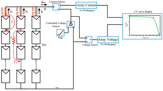
Figure 1.
Modeling and schematic of photovoltaic (PV) arrays in MATLAB/Simulink.
Numerous methods have been presented for the diagnosis of LL faults in the literature [7,8,9]. According to the approach that each method has adopted to identify faults, these methods can be divided into three categories.
The first category is a comparison between real and predicted parameters. For instance, in [10], a one-diode model was combined with an Exponentially Weighted Moving Average (EWMA) chart to investigate for any deviations from healthy conditions in PV systems. The difference between the measured and the predicted parameters is captured as residuals that are used as fault indicators. Dhimish et al. [11] presented a method based on the T-test statistical analysis, which used Voltage Ratio (VR) and Performance Ratio (PR) to specify the fault condition and the distinct faults, whereas the authors in [12] have used fuzzy-based decision making instead of the T-test. Moreover, there are a few methods that compare real-time parameters with their threshold limits. A threshold-based method by analysis of perturbation and observation (P&O) MPPT has been proposed in [13]. A fault diagnostic technique has been proposed in [14] based on the characteristics and magnitudes of the voltage waveform of each string in a PV array. This method requires two external sensors to collect data because two voltage transducers have been used in each string. In summary, the most important drawbacks in these methods are inaccurate estimation of the PV system model under different conditions and the dependence of these methods on the quality of the threshold limits.
The second category of LL fault detection is based on analysis of the output signals. In [15], a quickest fault detection method was developed based on Autoregressive (AR) to detect variations in the output signals and the Generalized Local Likelihood Ratio (GLLR) test to check the faults. Kumar et al. [16] proposed a method based on wavelet packets. In this method, the array voltage change, the array voltage energy, and energy of the change in impedance were extracted as features by Discrete Wavelet Transform (DWT) and the threshold limits were used for detecting the faults. In order to extract features from the signals, these methods require extra hardware and software platforms. Therefore, they are very costly and difficult to implement.
Machine Learning (ML) is the third category, which is more accurate to detect and classify the faulty conditions in PV systems. For instance, a probabilistic neural network scheme was developed based on information from the manufacturer′s datasheet [17]. Garoudja et al. [18] studied an enhanced machine learning-based approach for fault diagnosis of PV systems by extraction of PV modules′ parameters. In [19], random forest learning is utilized as a kind of ensemble learning method. Two models have been developed by the C4.5 decision tree algorithm for fault detection and diagnosis in [20]. Lu et al. [21] developed a fault detection model for a PV system based on conventional neural networks and electrical time series graphs.
In general, little attention has been paid to LL faults under low mismatch or high-impedance in the aforementioned methods, which are the main challenges for detection and classification of LL faults in PV arrays. The studies [22,23,24] have tried to present multiple algorithms as an attempt to detect PV faults under these conditions. However, these methods also have two major drawbacks. First, these methods require a big dataset for the learning process, and another drawback of these methods is related to low accuracy in detecting the LL faults with high impedance or a low mismatch level.
To address the challenges discussed above, here, we propose two novel concepts to detect and classify the LL faults efficiently using a Support Vector Machine (SVM) classifier. The first concept has been developed via a Simulink-based model of PV arrays to extract the main features by analyzing characteristics of the Current–Voltage (I–V) curve under normal and LL fault conditions. In the second concept, a Genetic Algorithm (GA) has been applied to optimize the feature subset selection and SVM parameters in order to obtain a higher accuracy for classifying the LL faults. This method not only reduces the number of datasets required for the training of the SVM classifier, but also it improves the accuracy of LL fault detection and classification. The main contributions of this study are summarized as follows:
- The main features of the faults have been extracted from I–V characteristics of PV arrays using a Simulink-based model for distinguishing between faulty and normal conditions.
- To the best of our knowledge, for the first time, a Genetic Algorithm (GA) has been developed for feature selection and parameters of classifier optimization in fault detection and classification for PV systems. This algorithm has been implemented using Python.
- The proposed method is able to detect and classify LL under a wide range of critical situations, even under low-mismatch levels and high-impedances.
2. The Proposed Method
In this study, GA is used to simultaneously optimize the feature selection of I–V curves and also the parameters of SVM classifier in order to effectively apply the parameters and features to implement LL fault detection and classification models. It should be taken into account that the learning process requires a dataset of normal and fault events. To this end, the fault features are extracted by analyzing the I–V curves of the PV array under different scenarios to create the dataset. In this section, the process of the features′ extraction from I–V curves, developed algorithms, and architecture of the proposed method is discussed.
2.1. Feature Extraction
For PV systems, the faulty conditions are reflected in the I–V curve, which gives sufficient information about PV functionality. However, the fault diagnosis methods based on the I–V curve have a major difficulty; finding a proper pattern for distinguishing between faulty and normal conditions could be very complicated. Figure 2 shows the I–V curves under normal conditions, an LL fault with 10% mismatch and impedance of R = 10 Ω, an LL fault with 20% mismatch and without impedance, and an LL fault with 30% mismatch and impedance of R = 10 Ω. As illustrated in Figure 2, the I–V curves cannot be directly adapted for fault classification. This is because of the following two reasons:
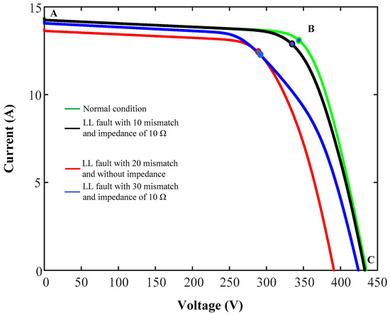
Figure 2.
Current–Voltage (I–V) curves under normal and line-to-line (LL) fault conditions at standard test condition (STC).
- I–V curves under normal conditions are close to LL faults at low mismatch levels with high impedances, which is a challenging task to identify the faulty conditions.
- I–V curves related to the LL faults under low mismatch and low impedances are very close to LL faults at high mismatch levels with high impedances, which is another challenge to classify the faulty conditions.
However, to distinguish the normal cases from the LL faults and also to classify LL fault events from each other, the detail processing of I–V curves is required. This processing includes efficient extracting of the features and also selecting the features for learning process of any type of faulty conditions. In this study, a PV array has been modeled in MATLAB software in order to simulate the faults and the normal events under various scenarios, see Figure 1. The PV array consists of 3 strings with 10 modules in each string. The detailed parameters of the PV modules (at STC) are listed in Table 1. The output voltage and current of the PV array are recorded by controlling the output value of the voltage source. Later, these values are transmitted to the MATLAB workspace to capture the I–V curves. In order to detect and classify accurately the faulty conditions, ten features have been extracted (see Table 2) from the I–V curves via analyzing the I–V characterization under normal and fault events based on three points, namely: short circuit current (A), Maximum Power Point (MPP) (B), and open-circuit voltage (C), (see Figure 2).

Table 1.
Simulated PV module parameters.
Table 2.
Extracted features from I–V characteristics of the PV array.
2.2. Developed Algorithms
2.2.1. Support Vector Machines (SVM)
SVM is a pattern recognition model that is applied for classification models. SVM classifiers have been successfully used to separate the data into two or several classes in many applications, especially fault detection in PV systems [24,25]. The major advantage of SVM classifiers is that they are resistant against the error of models and also have comparable computational efficiency with other machine learning methods. Hence, it can be used as a powerful model for detecting and classifying the LL faults in PV arrays. The SVM classifier aims to find a hyperplane in the feature space in order to properly separate data with a maximum margin. The closest data samples to the hyperplane are named “Support Vectors” [26].
To better understand the function of the SVM classifier, we briefly describe the SVM formulation in a binary classification problem. In the case of binary classification, a linear straight line can be a good hyperplane for separating data of each class with a maximum margin.
According to the training data , where records the category of the sample, and represents the input space vector, indicates the dimensional feature space, and n is the number of data instances. The linear hyperplane is expressed in Equation (1):
where b is a scalar and w is the weight vector.
Two important features for finding this hyperplane are: error in separating data must be minimal, and distance from the nearest data of each class should be maximum. Therefore, the search area for the hyperplane can be anywhere between support vectors. Hence, the SVM classifier for separable training data solves an optimization problem in order to maximize the distance value between the margins by finding the optimal hyperplane. Equation (2) describes the optimization problem:
It should be noted that it is challenging to specify an optimal hyperplane for non-separable cases that can accurately classify each training sample. The slack variable is introduced into the optimization problem in order to modify the non-separable to separable cases, presented in Equation (3):
where C is the penalty of misclassifying the training samples. This means that parameter C is a trade-off between the margin maximization and the classification error minimization. It should be noted that the bigger C causes more separation distance in the data samples. It can, however, also lead to an increase in the risk of generalization. In order to solve the optimization problem in Equation (3), Lagrange multipliers are introduced to transform the objective function into a dual form in Equation (4):
By solving Equation (4), the decision function for any data sample x specifies a label y. Equation (5) describes the decision function:
For training datasets that are not linearly separable, linear SVM cannot perform satisfactorily. To resolve this issue, nonlinear SVM is suggested. This means, the training samples are mapped into a higher-dimension by a kernel function, in which the samples are to be linearly separable. The corresponding kernel function and the final classification are defined in Equation (6):
This study uses the following kernel functions to select the best kernel for diagnosing the LL fault. These kernels are expressed in Equation (7):
2.2.2. Genetic Algorithm
The Genetic Algorithm (GA) is an evolutionary intelligent algorithm based on heuristic search algorithms. The GA was inspired by the theory of biological evolution, and it simulates the processes of natural selection mechanisms to find the optimal solutions [27]. The GA aims to achieve the evolution of the population via mutation, crossover, and natural selection. A solution produced by a GA is called a chromosome, which is made up of genes. Moreover, the set of chromosomes represents a population. In order to measure the suitability of the solution produced, the quality of these chromosomes is computed via a fitness function. Therefore, the chromosomes have a high chance of remaining in the next generation that has a higher fitness. Subsequently, to produce a new generation, some chromosomes in the population, called the parents, generate offspring through crossover operation, so that the parents′ chromosomes exchange some of their genes. Moreover, the genes of the new generation may be changed by mutation operation after crossover. It should be noted that crossover rate and mutation rate value control the number of intersected and mutated chromosomes [28].
A selection operation is employed to maintain the solution with the highest fitness. After several generations, the chromosome value will converge at the optimal solution for the problem. The procedure of the GA is given in the following steps [29]:
- Randomly generate the initial population.
- Evaluate the fitness value of each chromosome according to a fitness function.
- Perform the genetic operations including selection, crossover, mutations.
- The iteration is terminated if the terminating condition is met. Otherwise, return to step two.
2.3. The Parameter Optimization of the SVM and Feature Selection Based on GA
The structure of the proposed method is introduced in this subsection, including chromosome design, fitness function, and structure of the method.
2.3.1. Chromosome Design
In this study, in order to achieve a reliable model in detecting and classifying LL faults, all four kernels introduced in Section 2.2.1 are used to select the best kernel, and subsequently the parameters of each kernel are also optimized. However, it should be noted that we only need to tune one parameter in linear and polynomial kernels, namely parameter , whereas two parameters should be tuned in gaussian and sigmoid kernels i.e., and γ. Therefore, each chromosome is composed of three parts: parameters and γ, and also the feature subset. Figure 3 shows a binary string used in each chromosome.
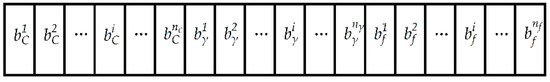
Figure 3.
Design structure of chromosome.
In Figure 3, indicates the misclassifying penalty , represents parameter γ in the kernel function, and shows the binary string of the feature subset. Moreover, and represent the number of the parameter , and the parameter γ, respectively. Note that and are determined based on the computational accuracy. In the binary code of the feature subset, specifies the number of features in the training dataset. Moreover, each binary bit in the feature subset can be “0” or “1”, in which “1” expresses that the corresponding feature has been selected to construct the model and “0” demonstrates that the corresponding feature has not been chosen.
2.3.2. Fitness Function
Fitness function is an important task of the proposed method. In order to obtain higher accuracy for the SVM classifier, the fitness function should be two attributes: the first one meets the requirements of high performance in the SVM classifier and the second one selects the number of features as infrequently as possible. This means, the higher fitness value represents the lesser number of features and shows a higher accuracy for the classifier. Therefore, in this study, we use a weighted combination of selected features with classification accuracy to construct a fitness function. The fitness function is expressed by Equation (8):
where denotes the classification accuracy weight, and refers to the weight of the feature subset. In object functions related to the feature subset, indicates the position related to the feature in the binary code of the feature subset, so that “0” means feature is not chosen; “1” means feature is chosen.
2.3.3. The Structure of the Proposed Method
In this research, GA has been used to optimize the SVM parameters and feature selection. Figure 4 illustrates the structure of the proposed method. The main steps are explained as follows:
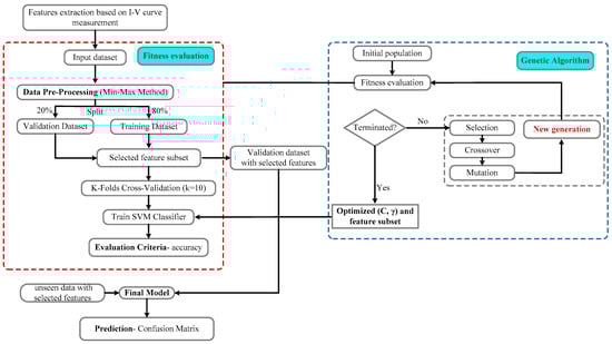
Figure 4.
System structure of the proposed method.
1. Data preprocessing:
Data preprocessing is an essential task in machine learning techniques for a variety of reasons. One of the most important aspects of data processing is data normalization because it can improve the cohesion among attributes existing in the dataset and improve the accuracy of the SVM classifier. Generally, each attribute will be normalized linearly in the range [0,1] by the Equation (9):
where is the scaled value, f is the original value, min refers to low bound of the feature value, and max denotes the upper bound of the feature value. After data preprocessing, the original dataset randomly splits into validation and training datasets. The training dataset is applied to build the SVM classifier while the validation dataset is applied to evaluate the learned SVM.
2. Setting the initial population:
Generally, the initial population is randomly produced. As previously mentioned, a binary string model is employed to specify initial chromosomes and tune the parameters, which include mutation rate, crossover rate, the number of iterations, the size of the population, etc. In this study, we randomly produce parameters and γ, whereas we choose all the features.
3. Fitness evaluation:
The training dataset is applied for learning the SVM classifier with the optimized feature subset and the obtained parameters γ and C. Moreover, this dataset is used for computing the classification accuracy. After this step, each chromosome is assessed by fitness function according to Equation (8).
4. Genetic operations:
Genetic operations consist of mutation, crossover, and selection, which are used to produce the new generation according to the fitness value. It should be taken into account that this leads to population diversity for providing a reliable solution.
5. Termination criteria:
The process ends if the criteria for termination are met. Subsequently, the feature subset and the optimal parameters γ, C are obtained. If this is not so, the process will continue with the next generation.
3. Results
3.1. Simulation Setup
In this paper, a simulation study has been carried out to evaluate the performance of the proposed method. The simulation procedure consists of two stages, namely, the first one is related to creating the dataset and the second one aims to detect and classify the LL faults (see Figure 4). In the first stage, the simulation platform has been developed in MATLAB, which was used for I–V curve analysis in order to extract the features. To this end, as previously mentioned, a PV array has been built in a MATLAB/Simulink environment using the configuration presented in Figure 1, which includes 3 PV strings with 10 PV modules in each string. Therefore, to create the dataset, the LL faults and normal events are simulated under various conditions (see Section 3.2). After building the dataset, LL faults have been detected and classified using the SVM classifier. Here, in order to improve the accuracy of the LL fault diagnosis, two layers have been defined. The first layer identifies the fault condition, which is a binary classification problem, whereas the second layer classifies LL faults based on mismatch levels, which is a multi-class classification problem. In these two layers, several common assumptions have been considered as follows:
- (1)
- The original dataset is divided into two datasets, which include the training and validation dataset. The percentage of the dataset that is used to train the models is 80%, and 20% is held back as a validation dataset.
- (2)
- The Cross Validation (CV) technique has been used in the learning process of the SVM classifier in order to obtain a more reliable estimation for the classifier performance. In this study, the 5-fold CV process has been used to assess each layer.
- (3)
- The classification accuracy metric has been introduced to assess the performance of the layers, which is defined based on the confusion matrix, see Table 3 [30]. This metric is formulated as Equation (10):where TP (true positive) is the case for identification of a data sample correctly, TN (true negative) is the case for rejection of a data sample correctly, FP (false positive) represents the case which is incorrectly identified, and FN (false negative) is the case which is incorrectly rejected.
Table 3. The confusion matrix.
- (4)
- In this research, we have set the search range of parameter γ to [0.0001, 10], whereas parameter is in the range of 0.1 to 1000. Moreover, the parameters of the genetic algorithm have been tuned as follows: the population size of 100 is selected, the mutation rate and crossover rate are equal to 0.6 and 0.1, and the maximum iteration number is set to 30. It should be noted that the termination criterion is set to the generation number.
3.2. Data Acquisition System
In order to validate the performance of proposed method for a PV system, original and unseen datasets have been recorded as a combination of normal and faulty cases by simulating a PV array in the environment of MATLAB/Simulink according to Figure 1. LL faults and normal conditions have been simulated under numerous scenarios, including different environmental conditions, fault impedances, and various mismatch levels. Environmental conditions cover a wide range of irradiance and temperature changes, in which the irradiance range varies from 200 W/m2 to 1000 W/m2, and the temperature range is from 0 °C to 40 °C. Moreover, the range of fault impedance is set to [0 Ω, 25 Ω] with a step of 5 Ω, and the mismatch level varies from 10% to 50% with an increment of 10%. In this research, 433 normal conditions and 570 cases of LL faults have been recorded under the aforementioned scenario’s operation.
After completing the learning process, each layer has been tested by an unseen dataset. This dataset was recorded under different conditions and scenarios from the original dataset. These conditions are the combinations of irradiance levels (350, 550, and 850 W/m2), operation temperatures (4, 7, 12, 17, 22, and 27 °C), fault impedances (3, 7, 12, and 17 Ω), and the mismatch level varies from 10% to 50% with an increment of 10%. Therefore, 60 normal conditions and 120 cases of LL faults are obtained by simulation setup in order to make an accurate and reliable assessment of the trained model.
3.3. Detection and Classification of LL Fault
In this study, the genetic algorithm was used to find the best features and the best kernels parameters in SVM classifier for LL fault detection and classification. As mentioned in Section 3.1, two layers have been developed to detect and classify the LL faults in PV arrays. It should be noted that the learning process has been developed in Python software. The main aim of the proposed method is to detect and classify precisely LL faults with lowest selected features.
To train and validate these two layers, 1003 samples (433 normal, and 570 LL fault samples) have been recorded as an original dataset, in which all these samples have been used to train and validate the first layers, whereas 570 samples were used to train and validate the second layers. In addition, 180 samples (60 normal, and 120 LL fault samples) have been recorded for the testing of the layers, in which all of these samples were used to test the first layers, whereas 120 samples have been used to test the second layers. The task of the first layer is to identify LL faults. Hence, this layer is a binary classification including two class labels, namely first class (normal events) and second class (LL fault events). Moreover, 802 data samples of the total original dataset are randomly selected for training the first layer, while the remaining samples of the original dataset have been used to validate the layer. The second layer aims to classify LL fault events based on mismatch levels because the main difficulty of the classification process of these faults is while the LL fault has happened under a low mismatch percentage, especially 10% and 20% mismatching. Therefore, this layer is designed as a multiclass classification, so that it includes three class labels, namely first class (10%), second class (20%), and third class (>20%). Furthermore, in this layer, 456 samples for the training dataset and 114 samples for the validation dataset have been considered.
Table 4 shows the comparison of training results of kernel functions used in the SVM classifier for both layers. Figure 5 and Figure 6 show the convergence of kernel functions in the first and second layers, respectively. The number and name of selected features, the best pairs of parameters of (C, γ), running time, and classification accuracy for each kernel function are given in Table 4. K-fold CV has been applied to estimate the accuracy of each kernel function in the two layers. As shown in Table 3, the Gaussian kernel function achieves a higher classification accuracy in both layers with the lowest elected features in comparison to other kernel functions. In the first layer, the mean accuracy was 95.93, and the feature number was equal to 3. In addition, in the second layer, the mean accuracy of 97.51 has been obtained, and the feature number was equal to 2. It is worth mentioning that the time taken for the total evolution generation has been recorded as running time, which is a serious limitation in search algorithms. As shown in Table 4, on a commonly used 4-core CPU, the polynomial and linear kernel functions take a significantly shorter running time than the other two kernel functions. However, it should be noted that the sigmoid kernel function takes a lot of time.
Table 4.
The training results of both layers using the proposed method.
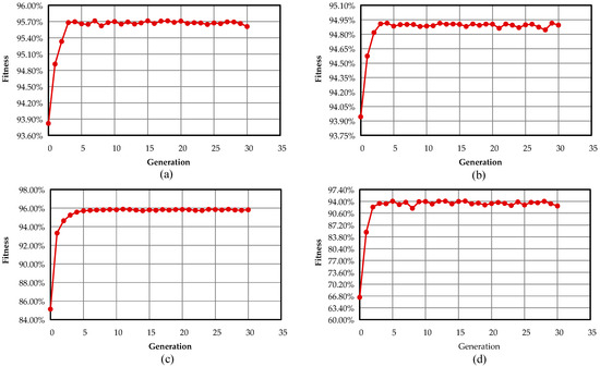
Figure 5.
Convergence curves of the kernel functions for the first layer: (a) the linear kernel; (b) the polynomial kernel; (c) the gaussian kernel; (d) the sigmoid kernel.
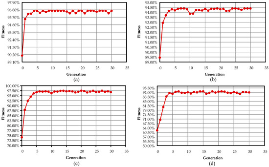
Figure 6.
Convergence curves of the kernel functions for the second layer: (a) the linear kernel; (b) the polynomial kernel; (c) the gaussian kernel; (d) the sigmoid kernel.
For further verification of the proposed method, the fitness value convergence curves of four kernel functions, which are used in the SVM classifier, have been plotted, as shown in Figure 5 and Figure 6. The horizontal axis indicates the number of generations, while the vertical axis represents the fitness function value. In the first layer, it is observed that the convergence speed of the Gaussian kernel function is almost lower than the other three kernel functions, but it has much less oscillation around the optimal solution. In the second layer, it can be observed that the optimal solution of kernel functions has been obtained after five generations. These results illustrate that all kernel functions in both layers are able to escape the local optimum. Moreover, the results have demonstrated that the convergence speed of all kernel functions is appropriate for achieving the optimal solution.
To verify the proposed method precisely, these kernel functions with the best-selected parameters and features were evaluated using validation and unseen datasets. The validation and testing results are summarized in Table 5. We have used the confusion matrix to show the performance of these kernel functions. As reported in Table 5, the Gaussian kernel function in both layers has shown that this model is able to detect and classify LL faults under low mismatch levels and high impedances with higher accuracy compared to other kernel functions.
Table 5.
Evaluation results of the proposed method using validation and unseen datasets.
4. Conclusions
In recent years, many efforts have been devoted to developing various methods for detecting and classifying the Line-to-Line (LL) faults. In some of these methods, little attention has been paid to the presence of fault impedances or the mismatch levels, which are the main challenges in diagnosing this type of faults. However, only a few studies have considered these two important conditions but they could not accurately detect and categorize the LL faults. In this study, a novel intelligent and autonomous method was proposed to detect and classify LL faults precisely. This proposed method has two main stages. In the first stage, the key features were extracted through analyzing the I-V characteristics under various LL fault events and normal operation. In the second stage, a genetic algorithm (GA) was used for parameter optimization of the kernel functions used in the Support Vector Machine (SVM) classifier and feature selection in order to increase the prediction accuracy and diminish the required training dataset to build the SVM model. The main aim of this study was to achieve a small training dataset for the learning process and also obtain a higher accuracy in LL fault detection and classification in the different situations, including low mismatch level and high fault impedance. In this study, the Gaussian kernel function has obtained the highest accuracy with the lowest selected features in both detection and classification processes. In this study, four kernel functions, namely, linear, polynomial, Gaussian, sigmoid, were also applied in the SVM models related to detection and classification of LL faults in order to select the best kernel. The results have demonstrated that the linear and Gaussian kernels have a higher performance compared to the other two kernel functions. However, the Gaussian kernel function has obtained the highest accuracy with the lowest selected features in both detection and classification processes. This kernel function has obtained an average accuracy of 96% and 97.5% in the learning process of detection and classification models, respectively. It should be noted that the number of the selected features is equal to three and two for detection and classification models, respectively. This proves the high capability of Gaussian kernels in the diagnosis of LL faults with the lowest necessary features. So, the proposed method was able to detect and classify various types of LL faults with an accuracy of around 97%.
The proposed method has provided various novel approaches for the autonomous monitoring of PV systems. In future work, we plan to validate the proposed method by experimental measurement.
Author Contributions
Conceptualization, invention, investigation, simulation, visualization and writing—A.E.; Conceptualization, invention, validation and supervision—J.M.; Conceptualization, invention, investigation, validation, visualization, writing, editing and supervision—M.A.; Reviewing, writing and editing—A.H.M.E.R. All authors have read and agreed to the published version of the manuscript.
Funding
This research received no external funding.
Acknowledgments
We like to acknowledge the COST Action CA16235 PEARL PV, Working Group 2 (WG2) for supporting this research.
Conflicts of Interest
The authors declare no conflict of interest.
References
- Leva, S.; Aghaei, M. Failures and Defects in PV Systems Review and Methods of Analysis. In Power Engineering Advances and Challenges Part B: Electrical Power; Taylor & Francis Group, CRC Press: Boca Raton, FL, USA, 2015; pp. 56–84. [Google Scholar]
- Aghaei, M.; Grimaccia, F.; Gonano, C.A.; Leva, S. Innovative Automated Control System for PV Fields Inspection and Remote Control. IEEE Trans. Ind. Electron. 2015, 62. [Google Scholar] [CrossRef]
- Mellit, A.; Tina, G.M.; Kalogirou, S.A. Fault detection and diagnosis methods for photovoltaic systems: A review. Renew. Sustain. Energy Rev. 2018, 91, 1–17. [Google Scholar] [CrossRef]
- Zhao, Y.; De Palma, J.F.; Mosesian, J.; Lyons, R.; Lehman, B. Line-line fault analysis and protection challenges in solar photovoltaic arrays. IEEE Trans. Ind. Electron. 2013, 60, 3784–3795. [Google Scholar] [CrossRef]
- Alam, M.K.; Khan, F.; Johnson, J.; Flicker, J. A Comprehensive Review of Catastrophic Faults in Mitigation Techniques. IEEE J. Photovoltaics 2015, 5, 982–997. [Google Scholar] [CrossRef]
- Pillai, D.S.; Rajasekar, N. A comprehensive review on protection challenges and fault diagnosis in PV systems. Renew. Sustain. Energy Rev. 2018, 91, 18–40. [Google Scholar] [CrossRef]
- Eskandari, A.; Milimonfared, J.; Aghaei, M.; de Oliveira, A.K.V.; Rüther, R. Line-to-Line Faults Detection for Photovoltaic Arrays Based on I-V Curve Using Pattern Recognition. In Proceedings of the 46th IEEE PVSC, Chicago, IL, USA, 16–21 June 2019; Volume 10, pp. 2–4. [Google Scholar]
- Zhao, Y.; Yang, L.; Lehman, B.; De Palma, J.F.; Mosesian, J.; Lyons, R. Decision tree-based fault detection and classification in solar photovoltaic arrays. In Proceedings of the IEEE Applied Power Electronics Conference and Exposition—APEC, Orlando, FL, USA, 5–9 February 2012; pp. 93–99. [Google Scholar]
- Madeti, S.R.; Singh, S.N. A comprehensive study on different types of faults and detection techniques for solar photovoltaic system. Sol. Energy 2017, 158, 161–185. [Google Scholar] [CrossRef]
- Garoudja, E.; Harrou, F.; Sun, Y.; Kara, K.; Chouder, A.; Silvestre, S. Statistical fault detection in photovoltaic systems. Sol. Energy 2017, 150, 485–499. [Google Scholar] [CrossRef]
- Dhimish, M.; Holmes, V.; Mehrdadi, B.; Dales, M. Simultaneous fault detection algorithm for grid-connected photovoltaic plants. IET Renew. Power Gener. 2017, 11, 1565–1575. [Google Scholar] [CrossRef]
- Dhimish, M.; Holmes, V.; Mehrdadi, B.; Dales, M. Multi-layer photovoltaic fault detection algorithm. High Volt. 2017, 2, 244–252. [Google Scholar] [CrossRef]
- Pillai, D.S.; Rajasekar, N. An MPPT-based sensorless line-line and line-ground fault detection technique for pv systems. IEEE Trans. Power Electron. 2019, 34, 8646–8659. [Google Scholar] [CrossRef]
- Saleh, K.A.; Hooshyar, A.; El-Saadany, E.F.; Zeineldin, H.H. Voltage-Based Protection Scheme for Faults Within Utility-Scale Photovoltaic Arrays. IEEE Trans. Smart Grid 2018, 9, 4367–4382. [Google Scholar] [CrossRef]
- Chen, L.; Li, S.; Wang, X. Quickest fault detection in photovoltaic systems. IEEE Trans. Smart Grid 2016, 9, 1835–1847. [Google Scholar] [CrossRef]
- Kumar, B.P.; Ilango, G.S.; Reddy, M.J.B.; Chilakapati, N. Online fault detection and diagnosis in photovoltaic systems using wavelet packets. IEEE J. Photovolt. 2017, 8, 257–265. [Google Scholar] [CrossRef]
- Akram, M.N.; Lotfifard, S. Modeling and health monitoring of DC side of photovoltaic array. IEEE Trans. Sustain. Energy 2015, 6, 1245–1253. [Google Scholar] [CrossRef]
- Garoudja, E.; Chouder, A.; Kara, K.; Silvestre, S. An enhanced machine learning based approach for failures detection and diagnosis of PV systems. Energy Convers. Manag. 2017, 151, 496–513. [Google Scholar] [CrossRef]
- Chen, Z.; Han, F.; Wu, L.; Yu, J.; Cheng, S.; Lin, P.; Chen, H. Random forest based intelligent fault diagnosis for PV arrays using array voltage and string currents. Energy Convers. Manag. 2018, 178, 250–264. [Google Scholar] [CrossRef]
- Benkercha, R.; Moulahoum, S. Fault detection and diagnosis based on C4.5 decision tree algorithm for grid connected PV system. Sol. Energy 2018, 173, 610–634. [Google Scholar] [CrossRef]
- Lu, X.; Lin, P.; Cheng, S.; Lin, Y.; Chen, Z.; Wu, L.; Zheng, Q. Fault diagnosis for photovoltaic array based on convolutional neural network and electrical time series graph. Energy Convers. Manag. 2019, 196, 950–965. [Google Scholar] [CrossRef]
- Zhao, Y.; Ball, R.; Mosesian, J.; De Palma, J.F.; Lehman, B. Graph-based semi-supervised learning for fault detection and classification in solar photovoltaic arrays. IEEE Trans. Power Electron. 2015, 30, 2848–2858. [Google Scholar] [CrossRef]
- Yi, Z.; Etemadi, A.H. Fault detection for photovoltaic systems based on multi-resolution signal decomposition and fuzzy inference systems. IEEE Trans. Smart Grid 2016, 8, 1274–1283. [Google Scholar] [CrossRef]
- Yi, Z.; Etemadi, A.H. Line-to-line fault detection for photovoltaic arrays based on multiresolution signal decomposition and two-stage support vector machine. IEEE Trans. Ind. Electron. 2017, 64, 8546–8556. [Google Scholar] [CrossRef]
- Harrou, F.; Dairi, A.; Taghezouit, B.; Sun, Y. An unsupervised monitoring procedure for detecting anomalies in photovoltaic systems using a one-class Support Vector Machine. Sol. Energy 2019, 179, 48–58. [Google Scholar] [CrossRef]
- Gholami, R.; Fakhari, N. Support Vector Machine: Principles, Parameters, and Applications. In Handbook of Neural Computation, 1st ed.; Elsevier: Cambridege, MA, USA, 2017; ISBN 9780128113196. [Google Scholar]
- Holland, J.H. Adaptation in Natural and Artificial Systems: An Introductory Analysis with Applications to Biology, Control, and Artificial Intelligence; MIT press: Cambridge, MA, USA, 1992; ISBN 0262581116. [Google Scholar]
- Kramer, O. Genetic Algorithm Essentials; Springer: Cham, Switzerland, 2017; Volume 679, ISBN 331952156X. [Google Scholar]
- Mirjalili, S. Genetic algorithm. In Evolutionary Algorithms and Neural Networks; Springer: Cham, Switzerland, 2019; pp. 43–55. [Google Scholar]
- Pecht, M.G.; Kang, M. Machine Learning: Fundamentals. In Prognostics and Health Management of Electronics: Fundamentals, Machine Learning, and the Internet of Things; John Wiley & Sons: Hoboken, NJ, USA, 2019; pp. 85–109. ISBN 9781119515326. [Google Scholar]
© 2020 by the authors. Licensee MDPI, Basel, Switzerland. This article is an open access article distributed under the terms and conditions of the Creative Commons Attribution (CC BY) license (http://creativecommons.org/licenses/by/4.0/).