A Spectral-Aware Convolutional Neural Network for Pansharpening

Abstract

Pansharpening aims at fusing a low-resolution multiband optical (MBO) image, such as a multispectral or a hyperspectral image, with the associated high-resolution panchromatic (PAN) image to yield a high spatial resolution MBO image. Though having achieved superior performances to traditional methods, existing convolutional neural network (CNN)-based pansharpening approaches are still faced with two challenges: alleviating the phenomenon of spectral distortion and improving the interpretation abilities of pansharpening CNNs. In this work, we develop a novel spectral-aware pansharpening neural network (SA-PNN). On the one hand, SA-PNN employs a network structure composed of a detail branch and an approximation branch, which is consistent with the detail injection framework; on the other hand, SA-PNN strengthens processing along the spectral dimension by using a spectral-aware strategy, which involves spatial feature transforms (SFTs) coupling the approximation branch with the detail branch as well as 3D convolution operations in the approximation branch. Our method is evaluated with experiments on real-world multispectral and hyperspectral datasets, verifying its excellent pansharpening performance.

1. Introduction

Multiband optical (MBO) images, including multispectral (MS) and hyperspectral (HS) images, can provide higher spectral resolution than red, green and blue (RGB) images and panchromatic (PAN) images, which expands the difference of the target objects and increases their identifiability. Such characteristics can be used to improve the effectiveness of various image tasks such as change detection [1], classification [2], object recognition [3], and scene interpretation [4]. Among almost all of these tasks, MS or HS images with high spatial resolution are desired. However, physical constraints make it difficult to acquire high spatial resolution MBO (HR-MBO) images with a single sensor, which are with high spectral resolution and high spatial resolution simultaneously. One way to address this problem is to generate HR-MBO images by fusing low-spatial-resolution MBO (LR-MBO) images and the associated high-resolution PAN images which is usually called pansharpening.

Over the last decades, a variety of pansharpening methods have been proposed in the literature [5,6,7,8]. Often-used methods can be categorized into two main groups: component substitution (CS) methods and multiresolution analysis (MRA) methods. CS methods seek to replace a component of the LR-MBO image with the PAN image, usually in a suitable transformed domain. This class includes intensity–hue–saturation (IHS) [9,10], principal component analysis (PCA) [11,12,13], Band-Dependent Spatial-Detail (BDSD) [14], Gram–Schmidt (GS) [15], Gram–Schmidt adaptive (GSA) [16], Brovey transform (BT) [17,18], and partial replacement adaptive component substitution (PRACS) [19]. Although these methods preserve accurate spatial information, they are often characterized by high spectral distortion, as the spectral ranges of the PAN and MBO images overlap only partially. MRA approaches regard pansharpening as a detailed extraction and injection process under multiresolution decomposition. This group consists of decimated wavelet transform (DWT) [20,21], undecimated wavelet transform (UDWT) [22], à trous wavelet transform (ATWT) [23], and Laplacian pyramid (LP) [24,25,26] methods. Compared with CS-based approaches, methods belonging to the MRA class can achieve higher spectral fidelity, but unfortunately, they may exhibit spatial distortion.

Besides the abovementioned, other categorizations of pansharpening methods can also be identified. Matrix factorization (MF) methods refer to inferring a basis or dictionary of the spectral subspace by factorizing the LR-MBO image and the associated coefficients by involving the PAN image, which are then used to reconstruct the HR-MBO image. This type of method includes the nonnegative matrix factorization (NMF) [27] and coupled nonnegative matrix factorization (CNMF) [28]. Owing to simple factorization rules, MF methods are easy to implement and efficient. Bayesian approaches, following the Bayesian inference framework, involve prior knowledge about the expected characteristics of the pansharpened image to determine its posterior probability distribution and to thus draw the estimation. Different types of prior knowledge have been used to assign prior distributions for Bayesian designing [29,30,31]. This type of method attempts to include the fusion process within an interpretable framework and achieves a trade-off between spatial and spectral fidelity. Model-based optimization methods mainly rely on observation models between the ideal fused image and the observed data, which is generally posed as a problem of minimizing cost function through iterative optimization algorithms. Examples include the sparse representation-based (SR) approach [32,33], the compressive sensing-based fusion (CSF) technique [34], and the online coupled dictionary learning (OCDL) [35]. Compared with the aforementioned methods, the model-based optimization methods can achieve higher spatial and spectral precision in the fusion result. However, it is relatively complicated and time-consuming due to the iterative optimization process.

Recently, convolutional neural networks (CNNs) have witnessed a sudden surge of interest in image resolution enhancement tasks such as super-resolution [36] and pansharpening [37]. Pansharpening, to some degree, can be regarded as a super-resolution task, where pansharpening is generally a multiple input, single output problem, while in a traditional image, super-resolution is a single input, single output process. In [38], Dong et al. proposed a super-resolution CNN (SRCNN) to reconstruct high-spatial-resolution images directly from low-spatial-resolution images in an end-to-end manner. Following the basic thread of SRCNN, Masi et al. introduced CNN into pansharpening for the first time and proposed a pansharpening CNN (PNN) [39]. After that, Wei et al. designed a deep residual pansharpening neural network (DRPNN) [40] and He et al. proposed two detail injection-based pansharpening CNNs (DiCNNs), i.e. DiCNN1 and DiCNN2 [41].

Although the aforementioned CNN-based pansharpening methods achieve better performances than traditional methods, there are still two problems that have not been well resolved. First, most previous CNN-based methods do not focus on consideration of strong spectral correlations that occur in MS/HS data and thus may incur spectral distortion in the fusion results, which means that some spectra (or pixels) of the recovered high-resolution MS/HS images deviate from those of the ideal high-resolution MS/HS images. Second, most existing CNN-based methods treat pansharpening merely as a black-box process and lack clear interpretability. To deal with these problems, we propose a spectral-aware pansharpening neural network (SA-PNN) in this study. The major contributions of our work can be summarized as follows:

• We create a two-branch structure, including the detail branch and the approximation branch, in SA-PNN which coincides with the interpretation of a detailed injection. The detail branch, which originated from catenation of the LR-MBO image and the PAN image, mainly fulfills the spatial detail resolution, while the approximation branch, which inputs merely the LR-MBO image, collaborates with the detail branch to inject the details to yield the final HR-MBO image. Therefore, our SA-PNN follows the concept of detail injection, which is a routine that inspired many classical pansharpening methods and hence gains clear interpretability.
• We use a spectral-aware strategy in SA-PNN to alleviate spectral distortion. The strategy involves mainly two aspects. On the one hand, spatial feature transforms (SFTs) are for the first time introduced into the pansharpening task to adjust spectra of the processed data adaptively to the observed scene. On the other hand, 3D convolution operations are used in the approximation branch which naturally accommodate the data resolving along the spectral dimension. Since spectral-aware strategies are adopted in SA-PNN, spectral processing or prediction is strengthened; thus, spectral distortion is expected to be reduced.

The rest of this paper is organized as follows. Section 2 briefly introduces the related backgrounds. Section 3 describes the proposed SA-PNN model in detail. The experimental results and analyses are presented in Section 4. Finally, the conclusion is presented in Section 5.

2. Backgrounds

The goal of pansharpening is to recover HR-MBO images from observed low spatial resolution ones and the connected PAN images. It usually can be formulated as minimizing the loss function of expected square error:

$$\ell \left(\mathit{\theta }\right)=E\parallel \widehat{\mathbf{H}}{(·;\mathit{\theta })-\mathbf{Y}\parallel }_F^2,$$

(1)

where $\widehat{\mathbf{H}}$ stands for the mapping from the observed MS/HS image and the associated PAN image to the high-resolution image to be predicted, $\mathbf{Y}$ is the ideal high-resolution image, and $\mathit{\theta }$ denotes the parameters connected to a parametric structure. CNNs, as specific instantiations of artificial neural networks, can be used to learn the mapping $\widehat{\mathbf{H}}(·;\mathit{\theta })$ in an end-to-end fashion. In CNNs, postulates such as the limited receptive field and the spatial invariant weight (so-called weight sharing) are normally suggested. The response of a convolutional layer in a CNN can be given by the following:

$${\mathbf{Y}}_l=\phi ({\mathbf{W}}_l\ast {\mathbf{X}}_l+{\mathbf{B}}_l),$$

(2)

where * denotes the convolution operation; ${\mathbf{X}}_l$ and ${\mathbf{Y}}_l$ are the input and output of the lth layer, respectively; ${\mathbf{W}}_l$ and ${\mathbf{B}}_l$ are the weight and bias matrices, respectively; and $\phi (·)$ represents the activation function, for which the rectified linear unit (ReLU) is commonly used due to its ability to mitigate gradient vanishing and computational simplicity [42].

Owing to the 3D data arrangement of MS/HS images, two kinds of convolution operations can be involved in CNN-based pansharpening, i.e., 2D convolution and 3D convolution. When applied along spatial dimension, 2D convolution can extract spatial information in MS/HS images. However, 2D convolution is unable to effectively exploit the potential features among bands, i.e., the spectral information encoded in neighboring bands, due to the separated synthesis for each output band. In contrast, 3D convolution is realized by convolving a 3D kernel with a data cube, which is naturally suitable for extracting both the spatial information between neighboring pixels and the spectral correlation in adjacent bands simultaneously.

3. Proposed Method

In this section, we develop a novel pansharpening neural network, called SA-PNN, which not only has clear interpretability but also is able to effectively alleviate spectral distortion.

The overall structure of our SA-PNN is graphically shown in Figure 1. As can be observed, the network comprises two major branches. One is the detail branch which extracts spatial details; the other is the approximation branch to extract approximations which collaborate the detailed information from the detail branch to build the final HR-MBO image. The detail branch takes the stacked PAN image of size $H_P\times W_P$ and the LR-MBO image of size $H_M\times W_M\times C$ as its input while using 2D convolutions to fulfill convolutional layer operations, which is designed with PAN image being assumed to contain most of useful spatial details and 2D convolutions being able to effectively collect spatial information. In contrast, the approximation branch takes only the LR-MBO image as its input and distills spectral approximation which collaborates the detailed information yielded in the detail branch to produce the final HR-MBO image of size $H_P\times W_P\times C$. Since 2D convolutions are unable to effectively build representation along the spectral dimension, they thus may incur spectral distortion; in such an approximation branch, 3D convolutions are used in convolutional layers to strengthen the spectral processing. The detail branch and the approximate branch form the basis of the detailed injection-based structure of our SA-PNN.

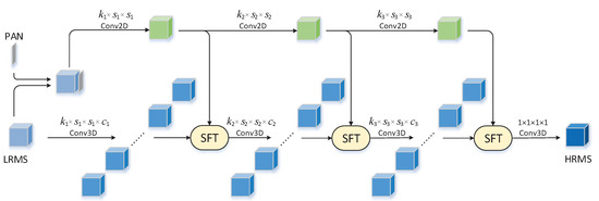
Figure 1. Overall structure of the spectral-aware pansharpening neural network (SA-PNN), which comprises a detail branch (green branch) and an approximation branch (blue branch).

Apart from the 3D convolution operation for convolution layers, the SFT strategy is also introduced in the approximate branch of SA-PNN (as show in Figure 1). SFT is originally designed to acquire the semantic categorical prior for color image enhancement [43]. We argue here that SFT can be used to adaptively adjust spectra in terms of the observed scene, to play a crucial role in the detail injection; and for the first time (to the best of our knowledge), to introduce it into pansharpening task. More specifically, in our SA-PNN, SFT provides an affine transformation for the convolutional feature maps based on a modulation parameter pair $(\alpha ,\beta )$, where $\alpha$ and $\beta$ are parameter maps conditioned on the observed scene. The transformation is carried out by a scaling and shifting operation as follows:

$$\mathbf{SFT}\left(\mathit{F}\right|\alpha ,\beta )=\alpha \odot \mathit{F}+\beta ,$$

(3)

where $\mathit{F}$ denotes the feature maps and ⊙ represents element-wise multiplication. As shown in Figure 2, for the lth layer in the approximation branch, we first obtain a modulation parameter pair $({\alpha }^l,{\beta }^l)$ from the feature maps of the lth convolutional layer ${\mathit{D}}^l$ (the lth green cube in Figure 2). Then, we apply the element-wise affine transformation to the feature maps ${\mathit{F}}^l$ (the lth blue cubes in Figure 2) according to (4):

$${\tilde{\mathit{F}}}_k^l={\alpha }_k^l\odot {\mathit{F}}_k^l+{\beta }_k^l,$$

(4)

where ${\alpha }_k^l$ and ${\beta }_k^l$ denote the kth modulation parameter pair at the lth layer, ${\mathit{F}}_k^l$ represents the kth feature map of the the approximate branch at the lth layer, and ${\tilde{\mathit{F}}}_k^l$ indicates the result after detail injection. It is noteworthy that both ${\alpha }_k^l$ and ${\beta }_k^l$ are 2D data while ${\mathit{F}}_k^l$ is volumetric data; thus, the operation in (4) actually applies the affine transformation to each band of ${\mathit{F}}_k^l$ according to the same parameter pair (${\alpha }_k^l$, ${\beta }_k^l$). As determined by the detail branch which carries high spatial details, ${\alpha }_k^l$ and ${\beta }_k^l$ carry spatial information in response to the observed scene. Therefore, with the calculation in (4), the feature map data are modulated spatially conditioned on the observed scene. As shown in Figure 1, undergoing a series of SFT operations, data cubes streamed in the approximation branch are spatially adjusted layer by layer and thus spectral processing is strengthened by spatial adaptiveness. With the detail injection being fulfilled layer-wise, a convolutional layer with a kernel in size $1\times 1\times 1$ is applied at the top of the network to yield the final HR-MBO image. As mentioned above, the parameter pair $(\alpha ,\beta )$ carries spatial information related to the observed scene and modulates the feature map data in the approximation branch according to (3) and (4). Intuitively, the modulation should be bidirectional, meaning that $\alpha$ and $\beta$ could be positive or negative. Therefore, the leaky ReLU (LReLU) [44] in the following

$$\mathbf{LReLU}\left(x\right)=\left\{\begin{array}{cc}x\hfill & x>0\hfill \\ ax\hfill & \mathrm{else},\hfill \end{array}\right.$$

(5)

rather than the standard ReLU is used in the relevant convolution layers yielding $\alpha$ and $\beta$ (as shown in Figure 2), where a is a positive constant.

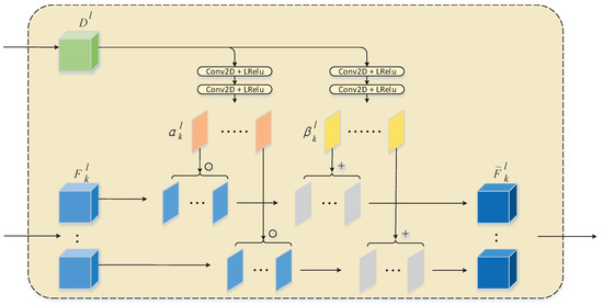
Figure 2. Spatial feature transforms (SFT) used in SA-PNN.

In brief, the proposed SA-PNN adopt a two-branch network structure, where one is the detail branch to be mainly responsible for spatial detail distilling while the other is the approximation branch to extract spectral-spatial information from the data and to fulfill injecting details with SFTs in a layer-wise manner; thus, SA-PNN has clear interpretability of the detail injection. Moreover, to strengthen the spectral processing to alleviate spectral distortion in the final pansharpening result, a spectral-aware strategy is developed which comprises SFTs and 3D convolutional layers jointly, where, especially SFTs can make spectra of the processed data to be automatically adjusted with respect to the observed scene.

4. Experiment Results

To evaluate the performance of our method, we conducted experiments on several real-world multispectral and hyperspectral image datasets and then made comparisons between SA-PNN and several representative pansharpening methods.

4.1. Experimental Setup

We carried out experiments on four dataset (three multispectral (MS) datasets acquired with the WorldView-2, IKONOS (the name comes from the Greek word $eik\overline{o}n$) [45], and Quickbird sensors and one hyperspectral (HS) dataset acquired with the Reflective Optics System Imaging sensors (ROSIS)). A brief description of these datasets is provided below.

• The WorldView-2 Washington dataset [46] comprises a high-resolution PAN image with a spectral range from $450\mathrm{nm}$ to $800\mathrm{nm}$ and an MS image with eight bands, including four standard colors (red, green, blue, and near-infrared) (1) and four new bands (coastal, yellow, red edge, and near-infrared) (2). The dimension of the PAN image is 24,800 × 23,600, whereas the size of the MS image is $6200\times 5900$. The spatial resolution of the PAN image is $0.46\mathrm{m}$ and that of the MS image is $1.84\mathrm{m}$ so that the resolution ratio R is 4. The radiometric resolution is 11 bits.
• The IKONOS Hobart dataset [47] contains a PAN image covering the spectral range from $450\mathrm{nm}$ to $900\mathrm{nm}$ and an MS image with four bands (blue, green, red, and near infrared). The dimension of the PAN image is 13,148 × 12,124 whereas the size of the MS image is $3287\times 3031$. The resolution ratio R is equal to 4 and the radiometric resolution is 11 bit, with the spatial resolution being $4\mathrm{m}$ for the MS image and $1\mathrm{m}$ for the PAN image.
• The Quickbird Sundarbans dataset [48] was obtained by the QuickBird sensor which provides a high-resolution PAN image with spatial resolution of $0.6\mathrm{m}$ and a four-band (blue, green, red, and near infrared) MS image with spatial resolution of $2.4\mathrm{m}$. The dimension of the PAN image is 15,200 × 15,200 while that of the MS image is $3800\times 3800$. The spectral range of the PAN image is from $450\mathrm{nm}$ to $900\mathrm{nm}$. The resolution ratio R is equal to 4, and the radiometric resolution is 11 bit.
• The Pavia University dataset [49] comprises a 103-band HS image covering a spectral range from $400\mathrm{nm}$ to $2500\mathrm{nm}$, with spatial resolution of $1.3\mathrm{m}$. The dimension of the HS image is $610\times 340$. Since the PAN image is absent, it is simulated by averaging the visible spectral bands of the HS image. The resolution ratio R for this dataset is usually manually set to 5 following the consensus in the pansharpening task, which means that the low-spatial-resolution HS image would be generated by degrading the original HS image with the scale factor of 5 in the subsequent experiments. The radiometric resolution is 13 bit.

We conduct experiments in the case of reduced-resolution assessments according to Wald’s protocol [50]. Specifically, the LR-MBO image degraded from the original MBO image will interpolate to the same spatial size as the degraded PAN image using a polynomial kernel (EXP) [51]. Subsequently, both of the pre-interpolated LR-MBO and degraded PAN image are used as the input of network, with the original MBO image as the ground truth. To demonstrate the superiority of the proposed SA-PNN model, several state-of-the-art CNN-based pansharpening methods are considered in our experiments for comparison, including PNN [39], DRPNN [40], and DiCNN1 [41]. In addition, several representative traditional methods, including PCA [11], GSA [16], PRACS [19], ATWT [23], Generalized Laplacian Pyramid with High-Pass Filtering (MTF-GLP-HPM) [26], CNMF [28], smoothing filter-based intensity modulation (SFIM) [52], guided filter PCA (GFPCA) [53], and Bayesian Sparse [54], are also run for comparison. Several widespread full-reference performance measures are used to evaluate pansharpening quality: average universal image quality index (Q) [55], x-band extension of universal image quality index (Qx) [56], spectral angle mapper (SAM) [57], Erreur Relative Globale Adimensionnelle de Synthèse (ERGAS) [58], root mean squared error (RMSE), and spatial correlation coefficient (SCC) [59].

4.2. Implementation Details

The methods mentioned before were trained on a laptop with an NVIDIA GeForce GTX 1060 GPU (CUDA 9.0 and CUDNN v7), an Intel^® Core${}^{\mathrm{TM}}$ i7-8750H CPU, and 16 GB RAM, using the Tensorflow framework and tested on MATLAB R2017b. The training set of each MS dataset consists of 12,800 patches with the size of $33\times 33$ and partial overlaps, which are cropped from a selected sub-scene. Analogously, the validation set consists of 3200 $33\times 33$ patches, which are cropped from another different sub-scene. In addition, a sub-image different from the training/validation set is selected for testing. For the HS dataset, the process of building the training/validation set is the same as that on the MS datasets except the size of the patches, which is only $11\times 11$, limited to the small size of this dataset. The sizes of convolutional kernels are empirically set to $7\times 7$ for the detail branch while are $7\times 7\times 3$ for the approximation branch. Also, the number of layers in our SA-PNN is empirically set to 4. The batch size using in the training phase is 64. The initial learning rate is set to 0.00005, and it is reduced to half every ${10}^5$ iterations. The mean squared error (MSE) is chosen as the loss function and optimized with the Adam algorithm. The training process terminates at $5\times {10}^5$ iterations. Table 1 shows the average training time of our SA-PNN on four datasets under GPU mode. Note that the train time on the Pavia dataset is less than that on the other three datasets due to the smaller size of the training patches.

Table 1. Average training time on four datasets ($5\times {10}^5$ iterations).

Dataset	Training Time
WorldView-2	$84h$$38\min$
IKONOS	$52\mathrm{h}$$49\min$
Quickbird	$52\mathrm{h}$$25\min$
Pavia	$9\mathrm{h}$$18\min$

4.3. Experimental 1—WorldView-2 Washington Dataset

This dataset covers an urban area in Washington D.C., and we chose a sub-scene with $256\times 256$ pixels for testing.

Table 2 shows the results of the reduced resolution quality assessment on the WorldView-2 dataset. The best results are shown in bold. As we can see, PRACS and CNMF have worse ERGAS than other methods, which indicates the poor overall pansharpening quality. In contrast, ATWT and MTF-GLP-HPM achieve relatively high scores on all metrics. Other methods like PCA and GSA restore the spatial details to some degree, as reflected in the better SCC than EXP. However, they yield worse SAM, which is useful to quantify the spectral distortion. The CNN-based methods achieve better performance compared to the traditional methods. Among them, our proposed SA-PNN yields the best numeric assessment results, especially in the impressive performance gain of SAM.

Table 2. Quality indexes at reduced resolution on a $256\times 256$ sub-scene of the WorldView-2 dataset (best result is in bold).

	Q8	Q	SAM	ERGAS	SCC
Reference	1	1	0	0	1
EXP	0.6612	0.6658	7.3985	7.1582	0.5202
PCA	0.8910	0.8353	7.4365	5.1001	0.8532
GSA	0.8870	0.8774	7.6723	4.3403	0.8470
PRACS	0.8255	0.8211	7.4250	5.2171	0.7946
ATWT	0.8865	0.8884	6.9038	4.2476	0.8768
MTF-GLP-HPM	0.8914	0.8933	6.9649	4.0964	0.8863
CNMF	0.8372	0.8381	7.8598	5.1929	0.8753
PNN	0.9441	0.9450	5.3307	2.9946	0.9369
DRPNN	0.9460	0.9469	5.2403	2.9657	0.9400
DiCNN1	0.9463	0.9472	5.1949	2.9575	0.9405
SA-PNN	0.9527	0.9533	4.8667	2.7689	0.9500

Although the numerical indicators show the performance of our proposed method clearly, we also focus on visual inspection to find noticeable distortions that elude quantitative analyses. As shown in Figure 3, the results of the traditional methods suffer from some spatial blur, such as the area in the upper middle of the images in Figure 3. Among them, CNMF is characterized by severe spectral distortions, such as the lake region in the bottom left of the images in Figure 3. The results of the CNN-based methods are more similar to the ground truth and our SA-PNN exhibits an excellent quality both in spatial detail and spectral fidelity. What is noteworthy is that the result of PNN shows spectral distortion at the edge, which is caused by convolution without padding during the training phase. This is unnoticeable in the numerical indicators.

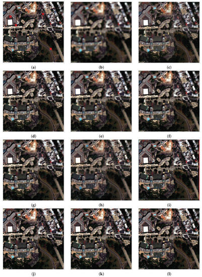
Figure 3. Pansharpening results for the WorldView-2 dataset: (a) ground truth; (b) polynomial kernel (EXP); (c) principal component analysis (PCA); (d) Gram–Schmidt adaptive (GSA); (e) partial replacement adaptive component substitution (PRACS); (f) à trous wavelet transform (ATWT); (g) Generalized Laplacian Pyramid with High-Pass Filtering (MTF-GLP-HPM); (h) coupled nonnegative matrix factorization (CNMF); (i) pansharpening CNN (PNN); (j) deep residual pansharpening neural network (DRPNN); (k) detail injection-based pansharpening CNN (DiCNN1); and (l) spectral-aware pansharpening neural network (SA-PNN).

To further compare performance, the spectral difference curves between the ground truth and the pansharpening results, which are generated by subtracting the ground truth from the pansharpening results, are plotted in Figure 4. Specifically, the values along the difference axes in Figure 4 indicate the difference in gray values between the ground truth and the pansharpening results. As we can see, while performance for individual spatial coordinates varies, on average, when examining multiple coordinates and bands, the spectral difference curves of SA-PNN closely approximate the reference, demonstrating that SA-PNN offers superior spectral fidelity.

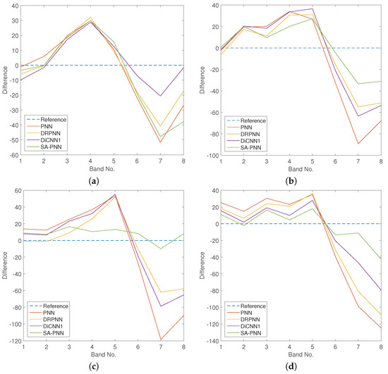
Figure 4. Spectral difference curves between the ground truth and the pansharpening results for the WorldView-2 dataset at randomly selected spatial coordinates: (a) (64, 32); (b) (53, 169); (c) (100, 55); and (d) (200, 202), which are marked in Figure 3a with red crosses.

4.4. Experimental 2—IKONOS Hobart Dataset

This dataset covers an urban area of Hobart in Australia. A sub-scene with $256\times 256$ pixels is used for testing in our experiments.

Table 3 shows the results of the reduced resolution quality assessment on the IKONOS dataset. The pansharpening qualities of various methods vary with the characteristics of the sensor. PCA and CNMF get worse pansharpening results compared to other methods. Unlike the results on the WorldView-2 dataset, GSA is much more preferable among the traditional methods. Such a phenomenon implies the poor robustness of the traditional methods. Similar to the previous dataset, CNN-based methods achieve a significant improvement. Among them, PNN achieves better results compared with DRPNN and DiCNN1, while our SA-PNN also achieves the best performance.

Table 3. Quality indexes at reduced resolution on a $256\times 256$ sub-scene of the IKONOS dataset (best result is in bold).

	Q4	Q	SAM	ERGAS	SCC
Reference	1	1	0	0	1
EXP	0.4654	0.4528	6.2444	6.0977	0.4811
PCA	0.6726	0.6689	6.2384	4.9672	0.7551
GSA	0.8094	0.8009	5.9050	4.2201	0.7643
PRACS	0.7715	0.7594	5.7972	4.3321	0.7652
ATWT	0.7625	0.7512	5.9945	4.4026	0.7649
MTF-GLP-HPM	0.7798	0.7698	5.9840	4.2576	0.7755
CNMF	0.6958	0.6565	5.9772	5.0231	0.7358
PNN	0.9273	0.9238	3.9546	2.6630	0.9214
DRPNN	0.9233	0.9188	4.0627	2.7367	0.9166
DiCNN1	0.9246	0.9204	4.0473	2.7168	0.9183
SA-PNN	0.9348	0.9313	3.6563	2.5401	0.9296

For visual inspection, Figure 5 shows the pansharpening results yielded by different methods. Similar to the conclusions drawn from Table 3, the results of the traditional methods are unsatisfactory for the spectral distortion and the diffused blur especially in the result of CNMF. Although the results of PNN, DRPNN, and DiCNN1 are superior in term of spatial details, they inevitably suffer from a little spectral distortion, e.g., the red roofs distributed in Figure 5. The result of our SA-PNN is more similar to the ground truth than others, with comparable spatial details and unnoticeable spectral distortion.

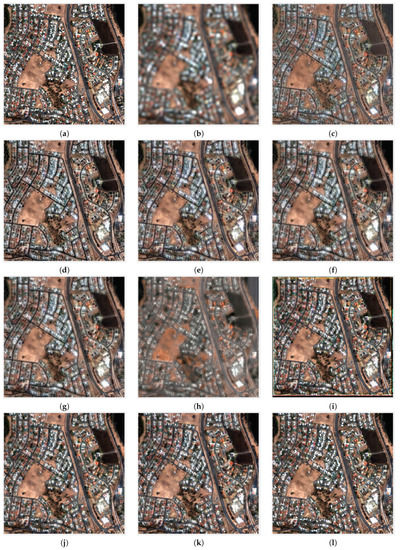
Figure 5. Pansharpening results for the IKONOS dataset: (a) ground truth; (b) EXP; (c) PCA; (d) GSA; (e) PRACS; (f) ATWT; (g) MTF-GLP-HPM; (h) CNMF; (i) PNN; (j) DRPNN; (k) DiCNN1; and (l) SA-PNN.

4.5. Experimental 3—Quickbird Sundarbans Dataset

This dataset covers a forest area of Sundarbans in India. Similar to the previous setting, a sub-scene with $256\times 256$ pixels was used for testing.

The results of the reduced resolution quality assessment on the Quickbird dataset are shown in Table 4. As the previous dataset, our SA-PNN still keeps being largely preferable. In the traditional methods, PCA and CNMF present worse pansharpening qualities while MTF-GLP-HPM gets the best result. PNN, DRPNN, and DiCNN1 achieve close improvements, which far exceed the traditional methods.

Table 4. Quality indexes at reduced resolution on a $256\times 256$ sub-scene of the Quickbird dataset (best result is in bold).

	Q4	Q	SAM	ERGAS	SCC
Reference	1	1	0	0	1
EXP	0.5914	0.5731	3.0248	2.8352	0.6693
PCA	0.7669	0.7055	3.0902	2.4352	0.8616
GSA	0.8747	0.8545	2.3774	1.7725	0.8954
PRACS	0.8370	0.8073	2.1989	1.7344	0.9023
ATWT	0.8685	0.8550	2.1692	1.6633	0.9064
MTF-GLP-HPM	0.8790	0.8674	2.0038	1.5398	0.9197
CNMF	0.6837	0.7198	2.7102	2.2655	0.8758
PNN	0.9414	0.9375	1.4584	1.0401	0.9669
DRPNN	0.9391	0.9360	1.4619	1.0505	0.9669
DiCNN1	0.9414	0.9385	1.4260	1.0340	0.9681
SA-PNN	0.9490	0.9465	1.3302	0.9715	0.9727

Visual inspection is shown in Figure 6. It is obvious that CNMF suffers from severe spectral distortion. Furthermore, the result of traditional methods are spatially blurred, such as the area in the upper right of the images in Figure 6. Analogously, CNN-based methods achieve better visual results and our SA-PNN still attained the best performance in terms of spatial detail reconstruction and spectral fidelity.

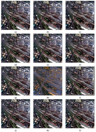
Figure 6. Pansharpening results for the Quickbird dataset: (a) ground truth; (b) EXP; (c) PCA; (d) GSA; (e) PRACS; (f) ATWT; (g) MTF-GLP-HPM; (h) CNMF; (i) PNN; (j) DRPNN; (k) DiCNN1; and (l) SA-PNN.

4.6. Experimental 4—Pavia University Dataset

This dataset covers a urban area in Pavia, northern Italy. Limited to the scant spatial size of the dataset, we choose a sub-scene with $150\times 75$ pixels for testing. Considering the large-volume data and the calculation efficiency, a dimensionality reduction operation is applied to this dataset when it is used in the CNN-based methods.

Table 5 presents the results of the reduced resolution quality assessment on the Pavia dataset. As we can see, although many traditional methods like GSA and Bayesian Sparse have better SCC than EXP, they are poor in guaranteeing the spectral fidelity due to the greatly increased number of bands. SFIM and MTF-GLP-HPM achieve relatively good performance. In the CNN-based methods, PNN gets high SCC while the other three metrics are very bad, which implies that PNN is not effective in improving spectral fidelity when used on data with a large number of bands. The results of DRPNN and DiCNN1 are competitive, with significant improvement compared to PNN. Our SA-PNN still achieved the best pansharpening quality.

Table 5. Quality indexes at reduced resolution on a $150\times 75$ sub-scene of the Pavia dataset (best result is in bold).

	SAM	ERGAS	RMSE	SCC
Reference	0	0	0	1
EXP	7.5634	6.9160	502.8104	0.8063
SFIM	6.8461	4.9617	404.0341	0.8831
CNMF	8.9287	6.0287	528.3205	0.8176
MTF-GLP-HPM	6.7015	4.6096	391.0704	0.8934
GSA	10.0496	5.6724	440.2654	0.8867
GFPCA	9.8152	7.3872	578.1234	0.7529
Bayesian Sparse	10.6064	5.4058	472.9086	0.8857
PNN	15.2681	9.8561	515.6730	0.9203
DRPNN	6.7640	4.2221	367.0981	0.9135
DiCNN1	6.8786	3.9914	343.6299	0.9230
SA-PNN	6.5109	3.9451	327.4077	0.9241

Visual inspection is also given in Figure 7. Obviously, the result of GFPCA is severely blurred while Bayesian Sparse shows spectral distortion such as the area in the upper left of the images in Figure 7. Other traditional methods like SFIM and CNMF achieve a trade-off between spatial details and spectral fidelity. Among all methods, our SA-PNN gets the best visual result.

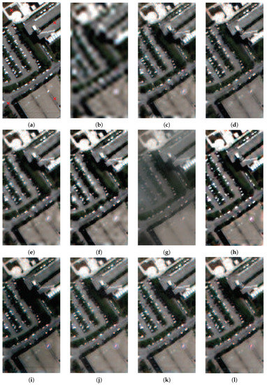
Figure 7. Pansharpening results for the Pavia dataset: (a) ground truth; (b) EXP; (c) SFIM; (d) CNMF; (e) MTF-GLP-HPM; (f) GSA; (g) GFPCA; (h) Bayesian Sparse; (i) PNN; (j) DRPNN; (k) DiCNN1; and (l) SA-PNN.

Considering that the simulated pseudo-color visual results shown in Figure 7 may not fully exhibit the spectral characteristics of the data with a large number of bands, for the CNN-based methods, we also show the spectral difference curves at randomly selected spatial coordinates: (8, 27), (8, 125), (64, 11), and (68, 131) in Figure 8. It is obvious that the spectral difference curves of PNN deviate heavily from the reference line, which corresponds to the spectral distortion presented in the pansharpening result of PNN. The overall spectral difference curves of our SA-PNN are the most approximate to the reference line, which demonstrates the excellent spectral fidelity ability of our SA-PNN again.

Figure 8. Spectral difference curves between the ground truth and the pansharpening results for the Pavia dataset at randomly selected spatial coordinates: (a) (27, 68); (b) (125, 68); (c) (11, 12); and (d) (131, 8), which are marked in Figure 7a with red crosses.

5. Conclusions

In this paper, we proposed a novel pansharpening neural network, SA-PNN, for MS/HS images. The network comprised of two branches, the detail branch and the approximate branch, has clear interpretability of detail injection. Furthermore, a spectral-aware strategy is used in SA-PNN, which is composed of SFT operations and 3D convolutions to strengthen the spectral processing. Thus, our network offers potential to reduce spectral distortion in the final pansharpening result. The experimental results on real-world MS/HS images validated the remarkable performance of our SA-PNN method.

References

- Souza, C. Mapping forest degradation in the Eastern Amazon from SPOT 4 through spectral mixture models. Remote Sens. Environ. 2003, 87, 494–506. [Google Scholar] [CrossRef]
- Perumal, K.; Bhaskaran, R. Supervised classification performance of multispectral images. J. Comput. 2010, 2, 2151–9617. [Google Scholar]
- Mohammadzadeh, A.; Tavakoli, A.; Zoej, M.V.J. Road extraction based on fuzzy logic and mathematical morphology from pan-sharpened ikonos images. Photogramm. Rec. 2006, 21, 44–60. [Google Scholar] [CrossRef]
- Laporterie-Dèjean, F.; de Boissezon, H.; Flouzat, G.; Lefevre-Fonollosa, M.-J. Thematic and statistical evaluations of five panchromatic/multispectral fusion methods on simulated PLEIADES-HR images. Inf. Fusion 2005, 6, 193–212. [Google Scholar] [CrossRef]
- Vivone, G.; Alparone, L.; Chanussot, J.; Mura, M.D.; Garzelli, A.; Licciardi, G.A.; Restaino, R.; Wald, L. A Critical Comparison Among Pansharpening Algorithms. IEEE Trans. Geosci. Remote Sens. 2015, 53, 2565–2586. [Google Scholar] [CrossRef]
- Alparone, L.; Wald, L.; Chanussot, J.; Thomas, C.; Gamba, P.; Bruce, L. Comparison of pansharpening algorithms: Outcome of the 2006 GRS-S data fusion contest. IEEE Trans. Geosci. Remote Sens. 2007, 45, 3012–3021. [Google Scholar] [CrossRef]
- Ghassemian, H. A review of remote sensing image fusion methods. Inf. Fusion 2016, 32, 75–89. [Google Scholar] [CrossRef]
- Amro, I.; Mateos, J.; Vega, M.; Molina, R.; Katsaggelos, A.K. A survey of classical methods and new trends in pansharpening of multispectral images. EURASIP J. Adv. Signal Process. 2011, 2011, 1–22. [Google Scholar] [CrossRef]
- Carper, W.; Lillesand, T.; Kiefer, R. The use of intensity-hue-saturation transformations for merging SPOT panchromatic and multispectral image data. Photogramm. Eng. Remote Sens. 1990, 56, 459–467. [Google Scholar]
- Chavez, P.; Sides, S.; Anderson, J. Comparison of three different methods to merge multiresolution and multispectral data: Landsat TM and SPOT panchromatic. Photogramm. Eng. Remote Sens. 1991, 57, 295–303. [Google Scholar]
- Chavez, P.; Kwarteng, A. Extracting spectral contrast in landsat thematic mapper image data using selective principal component analysis. Photogramm. Eng. Remote Sens. 1989, 55, 339–348. [Google Scholar]
- Shettigara, V. A generalized component substitution technique for spatial enhancement of multispectral images using a higher resolution data set. Photogramm. Eng. Remote Sens. 1992, 58, 561–567. [Google Scholar]
- Shah, V.; Younan, N.; King, R. An efficient pan-sharpening method via a combined adaptive PCA approach and contourlets. IEEE Trans. Geosci. Remote Sens. 2008, 46, 1323–1335. [Google Scholar] [CrossRef]
- Garzelli, A.; Nencini, F.; Capobianco, L. Optimal MMSE pan sharpening of very high resolution multispectral images. IEEE Trans. Geosci. Remote Sens. 2008, 46, 228–236. [Google Scholar] [CrossRef]
- Laben, C.; Brower, B. Process for Enhancing the Spatial Resolution of Multispectral Imagery Using Pan-Sharpening. U.S. Patent 6,011,875, 4 January 2000. [Google Scholar]
- Aiazzi, B.; Baronti, S.; Selva, M. Improving component substitution pansharpening through multivariate regression of MS+Pan data. IEEE Trans. Geosci. Remote Sens. 2007, 45, 3230–3239. [Google Scholar] [CrossRef]
- Gillespie, A.; Kahle, A.; Walker, R. Color enhancement of highly correlated images. II. Channel ratio and ”chromaticity” transformation techniques. Remote Sens. Environ. 1987, 22, 343–365. [Google Scholar] [CrossRef]
- Tu, T.; Su, S.; Shyu, H.; Huang, P.S. A new look at IHS-like image fusion methods. Inf. Fusion 2001, 2, 177–186. [Google Scholar] [CrossRef]
- Choi, J.; Yu, K.; Kim, Y. A New Adaptive Component-Substitution-Based Satellite Image Fusion by Using Partial Replacement. IEEE Trans. Geosci. Remote Sens. 2011, 49, 295–309. [Google Scholar] [CrossRef]
- Khan, M.; Chanussot, J.; Condat, L.; Montanvert, A. Indusion: Fusion of multispectral and panchromatic images using the induction scaling technique. IEEE Geosci. Remote Sens. Lett. 2008, 5, 98–102. [Google Scholar] [CrossRef]
- Otazu, X.; Gonzàlez-Audìcana, M.; Fors, O.; Núñez, J. Introduction of sensor spectral response into image fusion methods. Application to wavelet-based methods. IEEE Trans. Geosci. Remote Sens. 2005, 43, 2376–2385. [Google Scholar] [CrossRef]
- Nason, G.; Silverman, B. The stationary wavelet transform and some statistical applications. Wavelets Stat. Lect. Notes Stat. 1995, 103, 281–300. [Google Scholar]
- Vivone, G.; Restaino, R.; Dalla Mura, M.; Licciardi, G.A.; Chanussot, J. Contrast and error-based fusion schemes for multispectral image pansharpening. IEEE Geosci. Remote Sens. Lett. 2014, 11, 930–934. [Google Scholar] [CrossRef]
- Burt, P.; Adelson, E. The laplacian pyramid as a compact image code. IEEE Trans. Commun. 1983, 31, 532–540. [Google Scholar] [CrossRef]
- Lee, J.; Lee, C. Fast and efficient panchromatic sharpening. IEEE Trans. Geosci. Remote Sens. 2010, 48, 155–163. [Google Scholar]
- Aiazzi, B.; Alparone, L.; Baronti, S.; Garzelli, A.; Selva, M. An MTF-based spectral distortion minimizing model for pan-sharpening of very high resolution multispectral images of urban areas. In Proceedings of the 2nd GRSS/ISPRS Joint Workshop Remote Sensing and Data Fusion URBAN Areas, Berlin, Germany, 22–23 May 2003; pp. 90–94. [Google Scholar]
- Lee, D.; Seung, H. Algorithm for non-negative matrix factorization. Adv. Neural Inf. Process. Syst. 2001, 13, 556–562. [Google Scholar]
- Yokoya, N.; Yairi, T.; Iwasaki, A. Coupled nonnegative matrix factorization unmixing for hyperspectral and multispectral data fusion. IEEE Trans. Geosci. Remote Sens. 2012, 50, 528–537. [Google Scholar] [CrossRef]
- Golipour, M.; Ghassemian, H.; Mirzapour, F. Integrating hierarchical segmentation maps with MRF prior for classification of hyperspectral images in a Bayesian framework. IEEE Trans. Geosci. Remote Sens. 2016, 54, 805–816. [Google Scholar] [CrossRef]
- Hardie, R.; Eismann, M.; Wilson, G. MAP estimation for hyperspectral image resolution enhancement using an auxiliary sensor. IEEE Trans. Image Process. 2004, 13, 1174–1184. [Google Scholar] [CrossRef]
- Molina, R.; Katsaggelos, A.; Mateos, J. Bayesian and regularization methods for hyperparameter estimation in image restoration. IEEE Trans. Image Process. 1999, 8, 231–246. [Google Scholar] [CrossRef]
- Wei, Q.; Bioucas-Dias, J.; Dobigeon, N.; Tourneret, J. Hyperspectral and multispectral image fusion based on a sparse representation. IEEE Trans. Geosci. Remote Sens. 2015, 53, 3658–3668. [Google Scholar] [CrossRef]
- Huang, B.; Song, H.; Cui, H.; Peng, J.; Xu, Z. Spatial and spectral image fusion using sparse matrix factorization. IEEE Trans. Geosci. Remote Sens. 2014, 52, 1693–1704. [Google Scholar] [CrossRef]
- Ghahremani, M.; Ghassemian, H. Compressed-Sensing-based pan-sharpening method for spectral distortion reduction. IEEE Trans. Geosci. Remote Sens. 2016, 54, 2194–2206. [Google Scholar] [CrossRef]
- Guo, M.; Zhang, H.; Li, J.; Zhang, L.; Shen, H. An online coupled dictionary learning approach for remote sensing image fusion. IEEE J. Sel. Top. Appl. Earth Obs. Remote Sens. 2014, 7, 1284–1294. [Google Scholar] [CrossRef]
- Shi, W.; Caballero, J.; Huszàr, F.; Totz, J.; Aitken, A.P.; Bishop, R.; Rueckert, D.; Wang, Z. Real-time single image and video super-resolution using an efficient sub-pixel convolutional neural network. In Proceedings of the IEEE Conference on Computer Vision and Pattern Recognition, Las Vegas, NV, USA, 27–30 June 2016; pp. 1874–1883. [Google Scholar]
- He, L.; Zhu, J.; Li, J.; Plaza, A.; Chanussot, J.; Li, B. HyperPNN: Hyperspectral Pansharpening via Spectrally Predictive Convolutional Neural Networks. IEEE J. Sel. Topics Appl. Earth Observ. Remote Sens. 2019, 12, 2092–3100. [Google Scholar] [CrossRef]
- Dong, C.; Loy, C.; He, K.; Tang, X. Learning a deep convolutional network for image super-resolution. In Proceedings of the European Conference on Computer Vision, Zurich, Switzerland, 6–12 September 2014; pp. 184–199. [Google Scholar]
- Masi, G.; Cozzolino, D.; Verdoliva, L.; Scarpa, G. Pansharpening by Convolutional Neural Networks. Remote Sens. 2016, 8, 594. [Google Scholar] [CrossRef]
- Wei, Y.; Yuan, Q.; Shen, H.; Zhang, L. Boosting the accuracy of multispectral image pansharpening by learning a deep residual network. IEEE Geosci. Remote Sens. Lett. 2017, 14, 1795–1799. [Google Scholar] [CrossRef]
- He, L.; Rao, Y.; Li, J.; Chanussot, J.; Plaza, J.; Zhu, J.; Li, B. Pansharpening via Detail Injection Based Convolutional Neural Networks. IEEE J. Sel. Topics Appl. Earth Observ. Remote Sens. 2019, 12, 1188–1204. [Google Scholar] [CrossRef]
- Nair, V.; Hinton, G. Rectified linear units improve restricted Boltzmann machines. In Proceedings of the International Conference on Machine Learning, Haifa, Israel, 21–25 June 2010; pp. 807–814. [Google Scholar]
- Wang, X.; Yu, K.; Dong, C.; Loy, C.C. Recovering realistic texture in image super-resolution by deep spatial feature transform. In Proceedings of the IEEE Conference on Computer Vision and Pattern Recognition, Salt Lake City, UT, USA, 18–22 June 2018; pp. 606–615. [Google Scholar]
- Maas, A.; Hannun, A.; Ng, A. Rectifier Nonlinearities Improve Neural Network Acoustic Models. In Proceedings of the International Conference on Machine Learning, Atlanta, GA, USA, 16–21 June 2013; p. 3. [Google Scholar]
- Available online: https://en.wikipedia.org/wiki/Ikonos (accessed on 8 August 2020).
- Available online: https://www.digitalglobe.com/resources/product-samples (accessed on 8 August 2020).
- Available online: http://www.isprs.org/data/default.aspx (accessed on 8 August 2020).
- Available online: http://glcf.umd.edu/data/quickbird/datamaps.shtml (accessed on 8 August 2020).
- Available online: http://www.ehu.eus/ccwintco/index.php/Hyperspectral_Remote_Sensing_Scenes (accessed on 8 August 2020).
- Wald, L.; Ranchin, T.; Mangolini, M. Fusion of satellite images of different spatial resolutions: Assessing the quality of resulting images. Photogramm. Eng. Remote Sens. 1997, 63, 691–699. [Google Scholar]
- Aiazzi, B.; Alparone, L.; Baronti, S. Context driven fusion of high spatial and spectral resolution images based on oversampled multiresolution analysis. IEEE Trans. Geosci. Remote Sens. 2002, 40, 2300–2312. [Google Scholar] [CrossRef]
- Liu, J. Smoothing filter-based intensity modulation: A spectral preserve image fusion technique for improving spatial details. Int. J. Remote Sens. 2000, 21, 3461–3472. [Google Scholar] [CrossRef]
- Liao, W.; Goossens, B.; Aelterman, J.; Luong, H.Q.; Pižurica, A.; Wouters, N.; Saeys, W.; Philips, W. Hyperspectral image deblurring with pca and total variation. In Proceedings of the Workshop on Hyperspectral Image and Signal Processing: Evolution in Remote Sensing, Gainesville, FL, USA, 25–28 June 2013; pp. 1–4. [Google Scholar]
- Wei, Q.; Dobigeon, N.; Tourneret, J. Bayesian fusion of multi-band images. IEEE J. Sel. Topics Signal Process. 2015, 9, 1117–1127. [Google Scholar] [CrossRef]
- Wang, Z.; Bovik, A. A universal image quality index. IEEE Signal Process. Lett. 2002, 9, 81–84. [Google Scholar] [CrossRef]
- Alparone, L.; Baronti, S.; Garzelli, A.; Nencini, F. A global quality measurement of pan-sharpened multispectral imagery. IEEE Geosci. Remote Sens. Lett. 2004, 1, 313–317. [Google Scholar] [CrossRef]
- Yuhas, R.; Goetz, A.; Boardman, J. Discrimination among semi-arid landscape endmembers using the spectral angle mapper (SAM) algorithm. JPL Publ. 1992, 4, 147–149. [Google Scholar]
- Wald, L. Data Fusion: Definitions and Architectures: Fusion of Images of Different Spatial Resolutions; Presses des MINES: Paris, France, 2002. [Google Scholar]
- Zhou, J.; Civco, D.; Silander, J. A wavelet transform method to merge Landsat TM and SPOT panchromatic data. Int. J. Remote Sens. 1998, 19, 743–757. [Google Scholar] [CrossRef]
© 2020 by the authors. Licensee MDPI, Basel, Switzerland. This article is an open access article distributed under the terms and conditions of the Creative Commons Attribution (CC BY) license (http://creativecommons.org/licenses/by/4.0/).