Classification of Hyperspectral In Vivo Brain Tissue Based on Linear Unmixing

Featured Application

This paper describes the application of linear unmixing to classify intraoperative hyperspectral images of in vivo brain tissue with a reduced computational cost compared to a machine learning approach without compromising precision.

Abstract

Hyperspectral imaging is a multidimensional optical technique with the potential of providing fast and accurate tissue classification. The main challenge is the adequate processing of the multidimensional information usually linked to long processing times and significant computational costs, which require expensive hardware. In this study, we address the problem of tissue classification for intraoperative hyperspectral images of in vivo brain tissue. For this goal, two methodologies are introduced that rely on a blind linear unmixing (BLU) scheme for practical tissue classification. Both methodologies identify the characteristic end-members related to the studied tissue classes by BLU from a training dataset and classify the pixels by a minimum distance approach. The proposed methodologies are compared with a machine learning method based on a supervised support vector machine (SVM) classifier. The methodologies based on BLU achieve speedup factors of ~459× and ~429× compared to the SVM scheme, while keeping constant and even slightly improving the classification performance.

1. Introduction

Hyperspectral imaging (HSI) is a non-destructive and non-contact optical technique used for multiple applications, such as agricultural and water resources’ control, food quality analysis, military defense, or forensic medicine [1,2,3,4,5]. Due to its great potential to distinguish among materials, even when they are similar to the naked eye, HSI has been used as a non-invasive diagnostic tool in medical imaging, especially as a navigation tool in surgical procedures and cancer detection [6,7]. HSI is a technology that combines conventional imaging and spectroscopy to simultaneously obtain the spatial and spectral information of a sample [8]. The hyperspectral (HS) images contain data at hundreds of wavelengths, providing more insight than conventional RGB images. Each pixel exhibits a continuous spectrum (radiance, reflectance, or absorbance), acting as a fingerprint or signature used to distinguish the chemical composition of a particular pixel [8]. These spectral signatures are used together with labeling or classifying the pixels in the HS image, where the main challenges are the high dimensionality of the datasets and limited training samples. Linear unmixing is an analysis method that decomposes the continuous spectrum in each pixel of an HS image into different pure spectral signatures (called end-members) and their concentrations (called abundances) by a linear mixing model [9]. The joint estimation of end-members and their abundances in an HS image is called blind linear unmixing (BLU) analysis [10]. BLU is a type of inverse problem, where the end-members are assumed to be common in the HS image, and the abundances are estimated for each pixel. In this sense, BLU can also be applied as a classification tool for HS images based on the estimated spectral profiles of the end-members and their abundances per pixel [11,12,13]. Hence, the main challenge in BLU applications is to maintain high accuracy in the labeling task, while maintaining a low computational cost. On the other hand, recent approaches in HS image classification have considered machine learning and deep learning as classification tools [14,15,16,17], but although the accuracy could be improved, the required computational cost has to be carefully evaluated for a prospective real-time application.

2. Background

The most basic approaches for BLU are principal component analysis (PCA) and independent component analysis (ICA) [18,19]. These two methodologies have been applied to identify cancer by using HSI and BLU algorithms in previous studies. In [20,21], PCA was considered to identify different types of cancer in anomalous cells and to distinguish between tumor and normal tissues of head and neck cancer. Meanwhile, ICA was suggested to perform the classification of colon tissue cells [22] and to detect the presence of keratinized tissues to identify oral cancer [23]. Nevertheless, neither algorithm, ICA and PCA, considers a joint non-negativity and normalized condition on the resulting end-members, so their formulations do not contribute to the end-members’ physical interpretation. Other popular methods for non-negative datasets, such as multivariate curve resolution (MCR) or non-negative matrix factorization (NNMF), were used to identify breast cancer cells in HS microscopic images [24] or head and neck cancer in in vivo animal HS images [25], respectively. Another recent proposal is the extended blind end-member and abundance extraction (EBEAE) methodology that can be used for BLU in non-negative datasets by considering linearly independent end-members and normalized abundances. This method was previously used for biomedical imaging applications, including m-FLIM (multi-spectral fluorescence lifetime imaging) for chemometric analysis in oral cavity samples, OCT (optical coherence tomography) for macrophage identification in post-mortem artery samples, and in vivo brain tissue classification by using HSI [26].

Previous works in cancer detection have employed different machine learning approaches to classify HS in vivo brain data [27,28,29], including supervised and unsupervised algorithms, as well as deep learning methods. In [27], the use of a spatial-spectral algorithm was presented, where the differentiation among tissues was performed by using a combination of supervised and unsupervised machine learning methods. Thus, the supervised stage was based on support vector machine (SVM) classifier, K-nearest neighbor (KNN) filtering, and fixed reference t-distributed stochastic neighbors embedding (FR-t-SNE) dimensional reduction, where the unsupervised stage relied on the hierarchical K-means clustering algorithm. These two methods were combined by using a majority voting approach. In [28], deep learning approaches were explored, evaluating a 2D-CNN (two-dimensional convolutional neural network) and a 1D-DNN (one-dimensional deep neural network) against the use of SVM-based approaches to classify the samples. The processing framework in [28] involved both deep learning methods (2D-CNN and 1D-DNN), which increased the accuracy in the detection of tumor tissue with respect to the results obtained by each independent method. Finally, in [29], different optimization algorithms were explored to identify the most relevant wavelengths for the tumor margin delineation in the HS in vivo brain images. This methodology based on optimization algorithms revealed that with only 48 bands, the accuracy of the classification was not affected with respect to the reference results.

In this context, linear unmixing by EBEAE is proposed to classify intraoperative HS images of in vivo brain tissue. The main goal is to develop alternative methods with accurate results, but requiring smaller training times compared to a supervised machine learning classifier (SVM-based algorithm). In this way, two methodologies are suggested that rely on identifying the characteristics of end-members related to the studied tissue classes by EBEAE. In the first one, by computing the minimum distance to the end-members’ class sets, each pixel is labeled in the HS image. Meanwhile, the second one tries to isolate first the class related to the external materials or substances present in the surgical scenario, and then, the remaining pixels are labeled with the minimum distance philosophy to the tissue end-members’ sets. Our proposals could lead to future personalized classification approaches executed intraoperatively in real time, employing calibration spectral signatures obtained directly from the current patient.

The notation used in this work is described next. Scalars, vectors, and matrices are denoted by italic, boldface lower-case, and boldface upper-case letters, respectively. An L-dimensional vector with unitary entries is defined as ${\mathbf{1}}_L$. For a vector $\mathbf{x}$, its transpose is represented by ${\mathbf{x}}^{\top }$, its l-th component by ${\left(\mathbf{x}\right)}_l$, and its Euclidean norm by $\parallel \mathbf{x}\parallel =\sqrt{{\sum }_l{\left(\mathbf{x}\right)}_l^2}$. For a set $\mathcal{X}$, $\mathrm{card}\left(\mathcal{X}\right)$ denotes its cardinality, i.e., the number of elements in the set. A vector $\mathbf{x}$ with independent and identically distributed (i.i.d.) Gaussian entries (zero mean and finite variance) is denoted as $\mathbf{x}\sim \mathcal{N}\left(\mathbf{0}\right)$.

3. Materials and Methods

In this section, we review the technical, clinical, and protocol details of the studied datasets of in vivo human brain HS images and their ground-truth maps for classification. Next, the pre-processing chain of the HS raw images is briefly outlined, which looks to homogenize and extract the relevant information in the datasets. The mathematical formulation of the studied BLU algorithm is also described, which relies on alternated least-squares and constrained optimization. To compare the proposed methodologies, an SVM-based algorithm is introduced with a supervised philosophy for tissue classification. Finally, some standard classification metrics are presented to quantify the performance of the analyzed algorithms.

3.1. In Vivo Human Brain HS Dataset

The in vivo human brain HS images were captured by using a customized intraoperative HS acquisition system developed in [30], which was part of the European project HELICoiD (HypErspectraL Imaging Cancer Detection) (618080) [31]. The system was formed by a push broom HS camera operating in the VNIR (visible and near-infrared) spectral range from 400 to 1000 nm (Hyperspec^® VNIR A-Series, Headwall Photonics Inc., Fitchburg, MA, USA); an illumination system based on a quartz tungsten halogen (QTH) lamp of 150 W with a broadband emission between 400 and 2200 nm; and a scanning platform to provide the necessary movement for the push broom scanning, capable of covering an effective area of 230 mm. The resulting HS cubes contained 826 spectral bands with a spectral sampling of 0.73 nm, a spectral resolution of 2–3 nm, and a spatial resolution of 128.7 μm. The HS cube had a maximum size of 1004 × 1787 pixels with a maximum image size of 129 × 230 mm, where each pixel represents a sample area of 128.7 × 128.7 μm. However, each HS image of the database was manually segmented according to the region of interest, where the exposed brain tissue (parenchymal tissue) was present. The segmented images had a minimum and a maximum of 298 × 253 pixels and 611 × 527 pixels, respectively.

The HS database employed in this study was composed by twenty-six images from sixteen adult patients, and it was described in [32]. Patients underwent craniotomy for resection of intra-axial brain tumor or another type of brain surgery during clinical practice at the University Hospital Doctor Negrin at Las Palmas de Gran Canaria (Spain). Eight different patients were diagnosed with grade IV glioblastoma (GBM) tumor, and eleven HS images of exposed tumor tissue were captured. The remaining patients were affected by other types of tumors or affected by other pathologies that required performing a craniotomy to expose the brain surface. Written informed consent was obtained from all participant subjects, and the study protocol and consent procedures were approved by the Comité Ético de Investigación Clínica-Comité de Ética en la Investigación (CEIC/CEI) of the University Hospital Doctor Negrin.

To acquire the HS images during the surgical procedures, it was necessary to follow the protocol established in [30]. Craniotomy and resection of the dura were performed, and the operating surgeon initially identified the approximate location of the normal brain and tumor (if applicable). The surgeons placed sterilized rubber ring markers on the surface of the brain, where the presence of tumor and normal tissue was identified based on preoperative imaging data. Once the markers were located, the imaging operator captured the HS image, and the clinical expert performed a biopsy of the tissue located within the tumor markers, sending the sample to a pathologist. By this analysis, the physician confirmed the presence or absence of the tumor by histopathological diagnosis and also determined the tumor type and grading.

The HS acquisition system was operated by an engineer in charge of positioning the HS camera over the exposed brain surface, controlling the illumination system, and setting the image size to be captured according to the size of the exposed brain surface. The environmental illumination in the operating room did not affect the capture process due to the strong and precise illumination system available in the acquisition system. However, the surgical lighthead had to be turned off during the acquisition procedure, since it could interfere with the acquisition system illumination. The operator must avoid unintentional movements of the acquisition system during the capture. In case of an unexpected movement, the acquisition process was repeated. At the beginning of the surgical procedure, dark and white reference images were captured to perform the HS image calibration as explained in the next section.

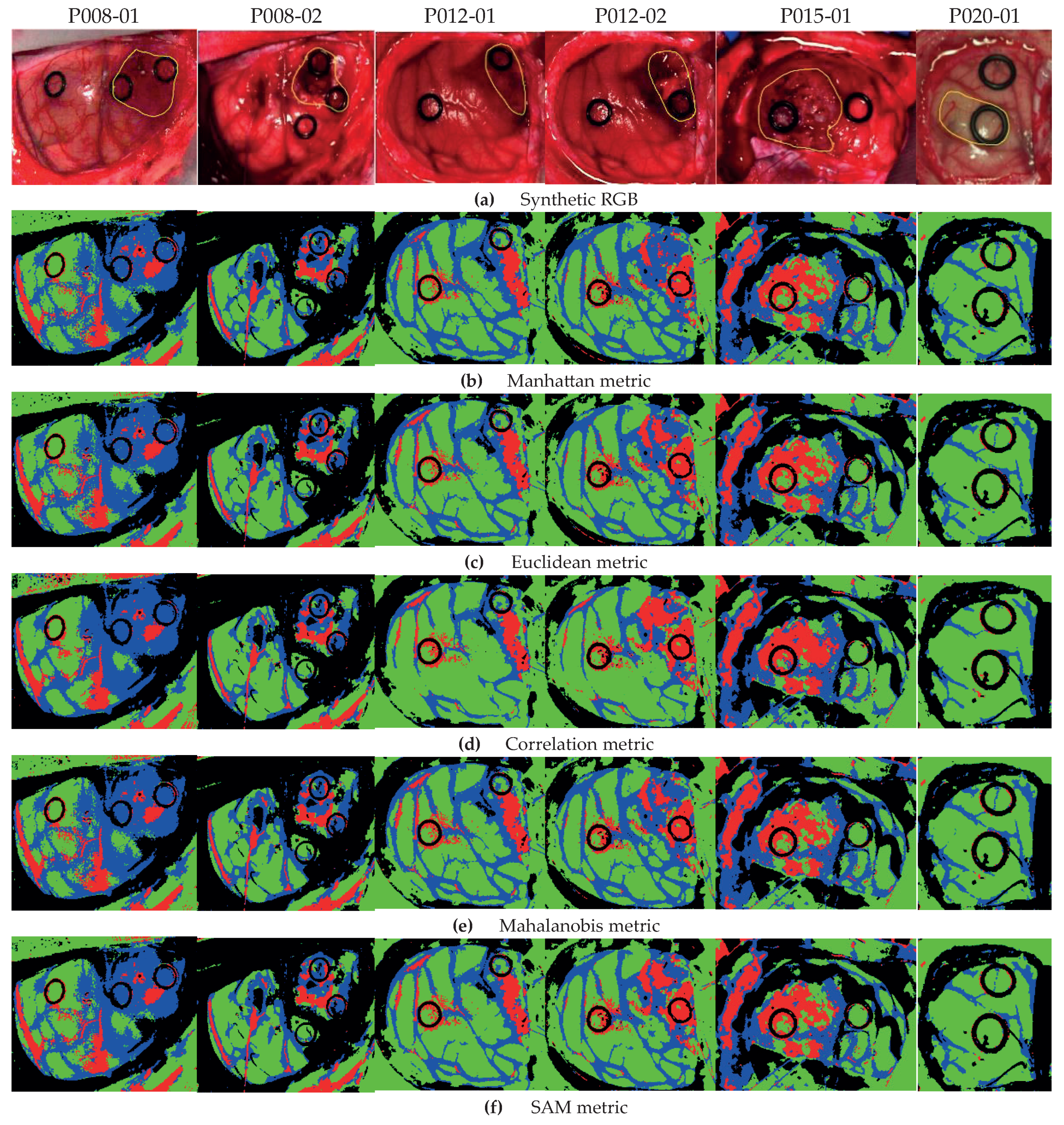
When possible, a first HS image was captured before tumor resection (e.g., P008-1 in Figure 1). After that, the HS acquisition system was moved out of the surgical area, and the tumor resection was performed by the surgeon. When the operating surgeon felt that it was safe to temporarily hold the surgery, a second HS image was captured while the tumor was resected (e.g., P008-2 in Figure 1). After acquiring the HS images, a specific set of pixels was labeled using a semi-automatic tool based on the spectral angle mapper (SAM) algorithm [33] developed in [32]. The surgeon, after completing the clinical procedure, selected only a few sets of very reliable pixels using the semi-automatic tool to create the ground-truth map for each captured HS image. After that, the SAM was computed in the entire image with respect to the pixel previously selected. Using a threshold manually established by experts, other pixels with the most similar spectral properties to the selected one could be identified. The pixels were labeled using four different classes: tumor tissue (TT), normal tissue (NT), hypervascularized tissue (HT) (mainly blood vessels), and background (BG). The background class involved other materials or substances present in the surgical scenario, but not relevant for the tumor resection procedure, such as skull bone, dura, skin, or surgical materials.

In this work, only GBM tumor pixels from four different patients were labeled from the eight patients originally affected by GBM tumor in this study, due to inadequate image conditions to perform the initial labeling. The remaining images with GBM tumor were included in the database, but no tumor samples were considered. In total, six HS images (P008-01, P008-02, P012-01, P012-02, P015-01, and P020-01) were labeled with the four studied classes (NT, TT, HT, and BG) and were employed as test datasets. The studied datasets can be observed in Figure 1, where in the synthetic RGB images, the tumor areas are surrounded by a yellow line, and the ground-truth maps of each HS image are shown below. Due to the low number of HS images with labeled tumor pixels, the leave-one-patient-out cross-validation methodology was proposed to evaluate the algorithms. In this methodology, the training dataset was composed by all patients’ samples except the one to be tested.

3.2. Data Pre-Processing

Before the classification step, each HS image was preprocessed. The HS image preprocessing chain was explained in [27,29] and consisted of four main steps: image calibration, spectral bands removal and selection, noise reduction, and normalization of spectral signatures. The first step was the HS image calibration, which was performed to smooth out the raw spectral signatures and to compensate for the nonlinear response of the HS camera. This step was carried out by using two reference images, the first one obtained on a white surface ($W_{ref}$) at the place where the clinical procedure was performed, with the same lighting conditions and the second acquired by taking a capture with the shutter closed, generating a dark reference image ($D_{ref}$). Once these two images were obtained, the preprocessed HS image $I(·)$ was computed by a normalization step at the k-th pixel ${\mathbf{y}}_k$:

$$I\left({\mathbf{y}}_k\right)=100\times \frac{R\left({\mathbf{y}}_k\right)-D_{ref}\left({\mathbf{y}}_k\right)}{W_{ref}\left({\mathbf{y}}_k\right)-D_{ref}\left({\mathbf{y}}_k\right)}k\in \{1,\dots ,K\},$$

(1)

where $R(·)$ is the raw HS image acquired from the HS camera and K is the number of pixels in the HS image.

In the second step, the spectral bands in the low and high frequency ranges were removed due to the high noise generated by the CCD sensor, producing low SNR in the first and last bands. For this reason, bands from 1 to 55 and from 700 to 826 were removed, resulting in an HS cube with 645 spectral bands that covered the spectral range from 440 to 902 nm. In a previous work [32], repeatability experiments were performed to demonstrate this statement. After this process, the spectral signatures were reduced by a 1:5 decimation procedure to avoid the redundant information between contiguous bands and also to reduce the execution time of the algorithms. Hence, each HS image was reduced to 128 spectral bands. The next stage involved a smoothing process by a Gaussian filter in the spectral domain. Finally, the last step in the preprocessing chain consisted of a normalization, also in the spectral domain, to avoid different radiation intensities produced by the non-uniform surface of the brain.

3.3. Extended Blind End-Member and Abundance Extraction

The methodology called extended blind end-member and abundance extraction (EBEAE), proposed in [26], allows estimating end-members and their abundances by a linear mixing model in non-negative datasets. In addition, the BLU process by EBEAE is controlled by hyperparameters that adjust the resulting similarity among end-members and the entropy of the abundances.

In the EBEAE formulation, there are $\widehat{K}$ non-negative and normalized (sum-to-one) pixels assumed for a certain class in the HS image. The spectral information in these pixels is expressed as an L-dimensional vector ${\mathbf{y}}_k\in {\mathbb{R}}^L$ with $k\in \{1,\dots ,\widehat{K}\}$. The set of labeled pixels is denoted as $\mathcal{Y}=\{{\mathbf{y}}_1,\dots ,{\mathbf{y}}_{\widehat{K}}\}$, and since the spatial information in the HS image is not relevant for the BLU process, the ordering in $\mathcal{Y}$ is indistinct. Each pixel is represented by a linear mixing model of order N ($2\le N<L$):

$${\mathbf{y}}_k=\sum _{n=1}^N{\alpha }_{k,n}{\mathbf{p}}_n+{\mathit{\eta }}_k=\underset{\mathbf{P}\in {\mathbb{R}}^{L\times N}}{\underbrace{\left[\begin{array}{ccc}{\mathbf{p}}_1& \cdots & {\mathbf{p}}_N\end{array}\right]}}\underset{{\mathit{\alpha }}_k\in {\mathbb{R}}^N}{\underbrace{\left[\begin{array}{c}{\alpha }_{k,1}\\ ⋮\\ {\alpha }_{k,N}\end{array}\right]}}+{\mathit{\eta }}_k=\mathbf{P}{\mathit{\alpha }}_k+{\mathit{\eta }}_k\forall k\in \{1,\dots ,\widehat{K}\},$$

(2)

where ${\mathbf{p}}_n\in {\mathbb{R}}^L$ is the n-th end-member, ${\alpha }_{k,n}\ge 0$ its abundance in the k-th pixel, and ${\mathit{\eta }}_k\in {\mathbb{R}}^L$ represents a noise or uncertainty vector (${\mathit{\eta }}_k\sim \mathcal{N}\left(\mathbf{0}\right)$). The EBEAE synthesis problem is defined as the following constrained optimization process:

$$\underset{\left\{{\mathit{\alpha }}_k\right\},\mathbf{P}}{min}J(\left\{{\mathit{\alpha }}_k\right\},\mathbf{P}),$$

(3)

where:

$$J(\left\{{\mathit{\alpha }}_k\right\},\mathbf{P})=\frac{1}{2\widehat{K}}\sum _{k=1}^{\widehat{K}}\frac{\left|\right|{\mathbf{y}}_k-\mathbf{P}{\mathit{\alpha }}_k{\left|\right|}^2}{\left|\right|{\mathbf{y}}_k{\left|\right|}^2}-\frac{\mu {\lambda }_{min}\left({\mathbf{P}}^{\top }\mathbf{P}\right)}{2\widehat{K}}\sum _{k=1}^{\widehat{K}}\left|\right|{\mathit{\alpha }}_k{\left|\right|}^2+\frac{\rho }{2\vartheta }\sum _{n=1}^{N-1}\sum _{j=n+1}^N\left|\right|{\mathbf{p}}_n-{\mathbf{p}}_j{\left|\right|}^2,$$

(4)

${\lambda }_{min}(.)$ represents the minimum eigenvalue of the argument matrix, $\mu \in [0,1)$ (entropy weight) and $\rho \ge 0$ (similarity weight) are hyperparameters, and:

$$\vartheta =\left\{\begin{array}{cc}(N-1)+\cdots +1\hfill & N\ge 3,\hfill \\ 1\hfill & N=2,\hfill \end{array}\right.$$

(5)

with restrictions ${\mathbf{1}}_N^{\top }{\mathit{\alpha }}_k=1$, ${\mathbf{1}}_L^{\top }{\mathbf{p}}_n=1$, and ${\mathit{\alpha }}_k,{\mathbf{p}}_n\ge 0$. Hence, the hyperparameters in EBEAE are defined as $(N,\mu ,\rho )$. To solve the optimization problem, an alternated least squares approach was used [34] to overcome the non-linear dependence of end-members ${\left\{{\mathbf{p}}_n\right\}}_{n=1}^N$ and abundances ${\left\{{\mathit{\alpha }}_k\right\}}_{k=1}^{\widehat{K}}$ in (4), until a convergence condition was met or a maximum number of iterations was exceeded [26]. In this formulation, the end-members ${\left\{{\mathbf{p}}_n\right\}}_{n=1}^N$ identify N characteristic or representative components to reproduce all the pixels in $\mathcal{Y}$.

3.4. Support Vector Machines Approach

The SVM strategy is a kernel-based supervised algorithm, which performs the classification by computing the probability of each pixel to belong to a certain class [35]. To compute the probability, the classifier calculates the best hyperplane that separates the data from different classes with a maximum margin. To do that, the hyperplane is computed by using a training dataset. In this sense, the SVM classifier was selected because it has shown good performance in HS data classification for medical applications [29,36]. The results obtained by the BLU-based approaches were compared with the SVM strategy to evaluate the classification performance and execution time. The LIBSVM package developed by Chang et al. [37] and MATLAB^® (R2019b, The MathWorks Inc., Natick, MA, USA) were employed for the SVM implementation, and the linear kernel with the default hyperparameters was used for the SVM configuration.

3.5. Classification Performance Metrics

The classification results were evaluated by comparing the studied approaches with the ground-truth datasets. Different metrics were selected for a quantitative evaluation to analyze classifiers that work well with unbalanced data. These metrics were: accuracy, sensitivity, specificity, F1-score, and the Matthews correlation coefficient (MCC) [38,39]. To compute these metrics, the following variables identify the possible outcomes in a binary classification problem:

• True positive ($TP$): both positive true value and classification result,
• False positive ($FP$): negative true value and positive classification result,
• True negative ($TN$): both negative true value and classification result.
• False negative ($FN$): positive true value and negative classification result.

As a result, the classification accuracy, sensitivity, specificity, F1-score, and MCC (normalized) are computed as:

$$\begin{array}{cc}\hfill \mathrm{accuracy}& =\frac{TP+TN}{TP+FP+TN+FN},\hfill \end{array}$$

(6)

$$\begin{array}{cc}\hfill \mathrm{sensitivity}& =\frac{TP}{TP+FN},\hfill \end{array}$$

(7)

$$\begin{array}{cc}\hfill \mathrm{specificity}& =\frac{TN}{TN+FP},\hfill \end{array}$$

(8)

$$\begin{array}{cc}\hfill \mathrm{F}1-\mathrm{score}& =\frac{2\times TP}{2\times TP+FN+FP},\hfill \end{array}$$

(9)

$$\begin{array}{cc}\hfill \mathrm{MCC}& =\frac{1}{2}\left(1+\frac{TP\times TN-FP\times FN}{\sqrt{(TP+FP)(TP+FN)(TN+FP)(TN+FN)}}\right).\hfill \end{array}$$

(10)

Accuracy, sensitivity, and specificity are common metrics in classification tasks that evaluate the precision with respect to positive and negative true values [38]. Meanwhile, the F1-score measures the precision of a test, where a value close to one means high precision and sensitivity [39]. The parameter MCC is used as a measure of the classification quality, and this parameter takes into account true and false positives together with negatives. The MCC is generally regarded as a balanced measure that can be used even if the classes are of very different sizes. In other words, the MCC(normalized) is a correlation coefficient between the observed and predicted binary classifications, returning a value between 0 and 1. A coefficient of 1 represents a perfect prediction, $0.5$ no better than a random prediction, and 0 total disagreement between prediction and observation [39].

4. Classification Methodology Based on Linear Unmixing

In the following sections, we propose two strategies for classifying the six in vivo brain tissue intraoperative HS images based on BLU by EBEAE. As previously described, in each HS image, some pixels were manually labeled by the clinical expert as four classes: NT, TT, HT, and BG, as ground-truth datasets. In fact, the BG class has a wide spectral range since it considers different materials or substances in the surgical scenario [27,29,30]. Hence, the rubber ring markers placed by the surgeon were part of the BG class. However, these rings had flat spectral signatures, which were pretty distinctive from the NT, TT, and HT classes. Therefore, to reduce the variability in the linear unmixing process by EBEAE, the rubber ring markers were segmented initially based on their flat spectral signatures (especially in the lower frequency bands) [29] and to avoid classification errors due to the rubber material, humidity, and light scattering. For this purpose, the energy in the initial twenty spectral signatures was collected, and the value was raised to the power of $3/2$ to enlarge the magnitude differences. The resulting image was normalized to grayscale tones. Finally, the Otsu method was applied to the grayscale image to segment the areas assigned to the rubber ring markers [40]. Next, two classification methodologies were explored in this work after this initial segmentation. The rationale behind these two methodologies was to use BLU to identify the most representative spectral signatures/end-members of the ground-truth datasets. Once these representative end-members were estimated, they were used to characterize each class studied at a lower dimension. To reduce the computational cost, each pixel was labeled by the minimum distance to the classes’ sets, which was feasible by the low dimension of these sets. The main difference from the second methodology was the assumption that an initial segmentation of the binary classes BG vs. no-BG (NT, TT, and HT) could improve the overall accuracy, without largely increasing the computation time. Next, these methodologies are explained in detail.

4.1. Method A

The first methodology consisted of three main stages after the segmentation of the rubber ring markers, which are illustrated in the block diagram of Figure 2. In the initial stage, the characteristic end-members of the four studied classes (NT, TT, HT, and BG) were estimated by the EBEAE algorithm [26]. This estimation process used as training information all the manually labeled pixels in the ground-truth datasets for the remaining five HS images (inter-patient approach). Thus, each labeled pixel in the EBEAE formulation was a vector gathering the 128 spectral bands (i.e., $L=128$). In each ground-truth dataset of the HS image, the number of labeled pixels was different, i.e., for each class, the number of measurements in the EBEAE procedure was variable.

For each class, the number of representative end-members was related to the variability of the spectral signatures in the dataset [27,30], and this parameter was selected by the procedure in [41]. The representative number of end-members was two for NT ($N_{NT}=2$), two for TT ($N_{TT}=2$), one for HT ($N_{HT}=1$), and three for BG ($N_{BG}=3$) for all HS images. Since for the HT class, only one end-member was needed, this was equivalent to using the average of the HT labeled ground-truth pixels. With respect to the hyperparameters of EBEAE, they were manually selected to improve the classification outcome, but following the guidelines in [26]. Thus, since the goal was to reduce the estimation error, the entropy weight was chosen always as zero ($\mu =0$). Meanwhile, the similarity weight $\rho$ should be small if there is large variability in the dataset. For this purpose, this hyperparameter was set as 0.3 for NT (${\rho }_{NT}=0.3$), 0.2 for TT (${\rho }_{TT}=0.2$), and 0.01 for BG (${\rho }_{BG}=0.01$). Consequently, after this estimation step, we had the sets of characteristic end-members $\{{\mathcal{P}}_{NT},{\mathcal{P}}_{TT},{\mathcal{P}}_{HT},{\mathcal{P}}_{BG}\}$ for the NT, TT, HT, and BG classes, respectively. In this way, we had low-dimensional sets for each class, i.e., $\mathrm{card}\left({\mathcal{P}}_{NT}\right)=2$, $\mathrm{card}\left({\mathcal{P}}_{TT}\right)=2$, $\mathrm{card}\left({\mathcal{P}}_{HT}\right)=1$, and $\mathrm{card}\left({\mathcal{P}}_{BG}\right)=3$.

As a second step, for the k-th pixel ${\mathbf{y}}_k$ in each HS image, the distance to each end-member set was computed by the concept of the distance from a point to a set [42], as:

$$d({\mathbf{y}}_k,{\mathcal{P}}_i)=\underset{\mathbf{p}\in {\mathcal{P}}_i}{inf}d({\mathbf{y}}_k,\mathbf{p})i\in \{NT,TT,HT,BG\},k\in \{1,\dots ,K\}$$

(11)

where $d(·,·)$ represents a distance or metric. In this study, five distances were evaluated:

$$\begin{array}{ccc}\hfill d_1(\mathbf{x},\mathbf{y})& =\sum _{l=1}^L\left|{\left(\mathbf{x}\right)}_l-{\left(\mathbf{y}\right)}_l\right|\hfill & \hfill \mathrm{Manhattan}\mathrm{metric}\end{array}$$

(12)

$$\begin{array}{ccc}\hfill d_2(\mathbf{x},\mathbf{y})& =\sqrt{{(\mathbf{x}-\mathbf{y})}^{\top }(\mathbf{x}-\mathbf{y})}\hfill & \hfill \mathrm{Euclidean}\mathrm{metric}\end{array}$$

(13)

$$\begin{array}{ccc}\hfill d_C(\mathbf{x},\mathbf{y})& =\frac{{\mathbf{x}}^{\top }\mathbf{y}}{\parallel \mathbf{x}\parallel \parallel \mathbf{y}\parallel }\hfill & \hfill \mathrm{Correlation}\mathrm{metric}\end{array}$$

(14)

$$\begin{array}{ccc}\hfill d_M(\mathbf{x},\mathbf{y})& =\sqrt{{(\mathbf{x}-\mathbf{y})}^{\top }\mathbf{Q}(\mathbf{x}-\mathbf{y})}\hfill & \hfill \mathrm{Mahalanobis}\mathrm{metric}\end{array}$$

(15)

$$\begin{array}{ccc}\hfill d_{SAM}(\mathbf{x},\mathbf{y})& ={cos}^{-1}\left(\frac{{\mathbf{x}}^{\top }\mathbf{y}}{\parallel \mathbf{x}\parallel \parallel \mathbf{y}\parallel }\right)\hfill & \hfill \mathrm{SAM}\mathrm{metric}\end{array}$$

(16)

where $\mathbf{Q}\in {\mathbb{R}}^{L\times L}$ represents the covariance matrix of the dataset. In the last stage, the k-th pixel ${\mathbf{y}}_k$ was classified according to the minimum distance among the four classes:

$$c\left({\mathbf{y}}_k\right)=arg\underset{i\in \{NT,TT,HT,BG\}}{min}d({\mathbf{y}}_k,{\mathcal{P}}_i).$$

(17)

4.2. Method B

For the second methodology (see Figure 3), the fundamental aspect was to make an accurate estimation of the BG class first, which presented the largest spectral variability [27,29]. Initially, the calculation of the representative end-members for each HS image followed the same procedure as in Method A. Then, the set of all estimated end-members is defined as:

$$\mathcal{P}={\mathcal{P}}_{NT}\cup {\mathcal{P}}_{TT}\cup {\mathcal{P}}_{HT}\cup {\mathcal{P}}_{BG}.$$

Next, for the k-th pixel ${\mathbf{y}}_k$ in the HS image, the distance to all $M=\mathrm{card}\left(\mathcal{P}\right)$ estimated end-members in $\mathcal{P}$ was computed. As a result, there were M images constructed by the distance to each characteristic end-member. These images were segmented by applying the K-means algorithm in the four different groups [43].

Now, by using the pixels labeled as no-BG (NT, TT, and HT) for each studied patient (intra-patient approach), the regions belonging to the BG class were selected by means of the positions of the spectral signatures of the no-BG class in the HS image. In this last step, a binary image was generated for the BG class, which was concatenated with the regions of the rubber ring markers to build the overall BG image for that patient. The pixels labeled as BG were discarded in the later stages. In the next step of Method B, the distance of the k-th pixel ${\mathbf{y}}_k$ outside the BG mask in the HS image was calculated to the end-members sets $\{{\mathcal{P}}_{NT},{\mathcal{P}}_{TT},{\mathcal{P}}_{HT}\}$ by (11). For the last stage, the k-th pixel ${\mathbf{y}}_k$ was classified according to the minimum distance in (17), but among only three classes $\{NT,TT,HT\}$.

5. Results and Discussion

In this section, we evaluate the performance of the proposed classification methodologies based on BLU by EBEAE, with respect to the SVM-based approach. We evaluate first the effect of different metrics in Method A, and next, we present the comparison results among Method A, Method B, and the SVM scheme.

5.1. Metrics’ Evaluation for the Distance to End-Members’ Sets

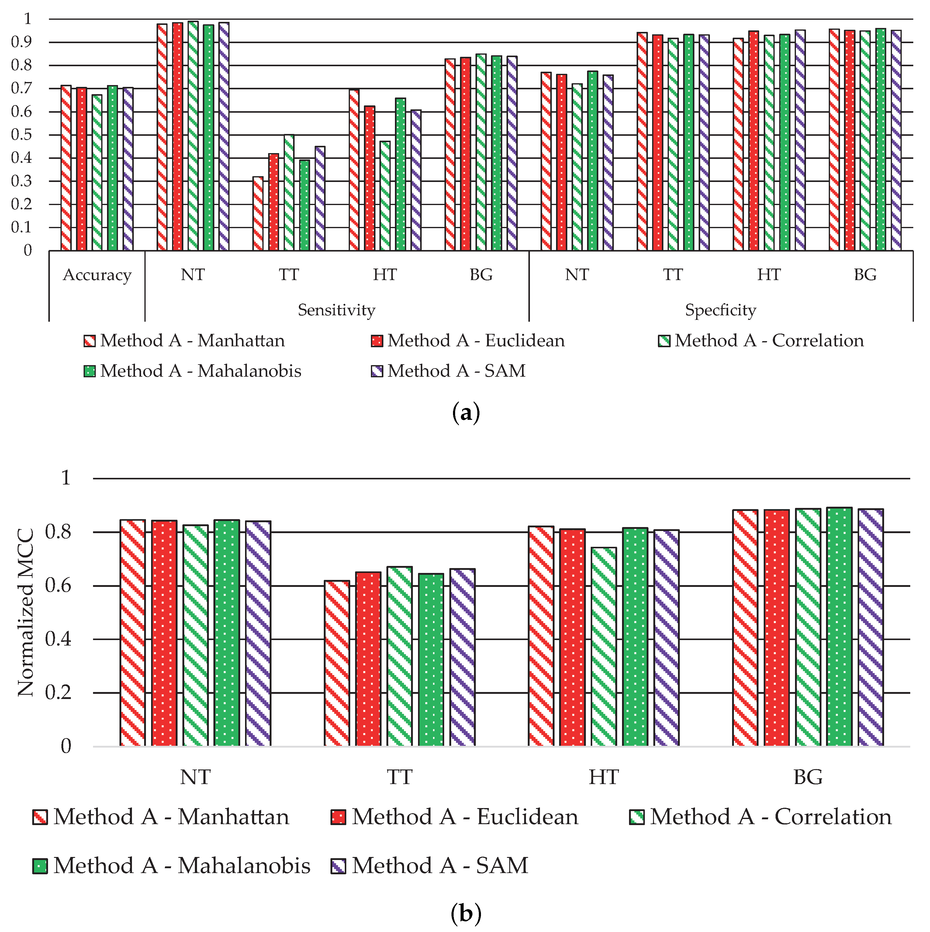
Method A is based on first detecting the rubber ring markers, used by the surgeon to identify tumor and healthy tissues, and then removing this information to estimate the characteristic end-members. The evaluation of this methodology was performed by using the six test HS images in Figure 1 (P008-01, P008-02, P012-01, P012-02, P015-01, and P020-01), and the different distances in Equations (12)–(16): Manhattan metric, Euclidean metric, correlation metric, Mahalanobis metric, and SAM.

Figure 4 shows the average performance classification results obtained for each metric. Figure 4a shows the accuracy, sensitivity, and specificity results, where the accuracy value is similar in all metrics. Besides that, the sensitivity performance for the NT and BG classes with all metrics is also equivalent. Meanwhile, the main performance differences are observed in the TT and HT classes. The classification with the Manhattan metric achieves the best sensitivity in the HT class with a value of ~70%, while the correlation metric offers the worst performance (~47%). However, related to the TT class, the correlation metric achieves the best sensitivity results (50%), and the worst performance is obtained by the Manhattan metric (~32%). Finally, the specificity results are mostly consistent in all classes; for the NT class, the performance is always higher than 70%, and higher than 90% for the TT, HT, and BG classes. Figure 4b shows the MCC results, where we observe that all metrics offer similar performance, except the correlation metric in the HT class, which exhibits a reduction of ~7% related to the best solution. However, this distance achieves the best result in the TT class. For this reason, the correlation metric provides on average the best results, especially highlighted in the TT class, being highly relevant due to the nature of our clinical application.

Figure 5 shows the classification maps obtained with each metric for Method A. Figure 5a illustrates the synthetic RGB images with the tumor area marked by a yellow line, and in Figure 5b–f are the results with all metrics in Equations (12)–(16).

As highlighted by the accuracy performance in Figure 4a, the classification is quite consistent with all metrics. Nonetheless, we obtain a better definition of the tumor areas in the HS images by using the correlation metric, for example in images P012-02 and P015-01. In particular, for image P012-02 with the Manhattan metric (Figure 5b), some HT pixels in the tumor area are misclassified; however, by using the correlation metric (Figure 5d), the tumor area is correctly identified. Furthermore, the correlation metric in the same image shows an homogeneous tumor area with respect to other distances. Note that for the P020-01 image, none of the metrics are able to distinguish the TT class, since the synthetic RGB image highlights that the marked tumor area presents a similar colorization to the NT class, which is consistent with the result in [29]. As stated in such previous work, this misclassification of the TT class could be produced by the lack of a more complete database that takes into account the inter-patient spectral variability.

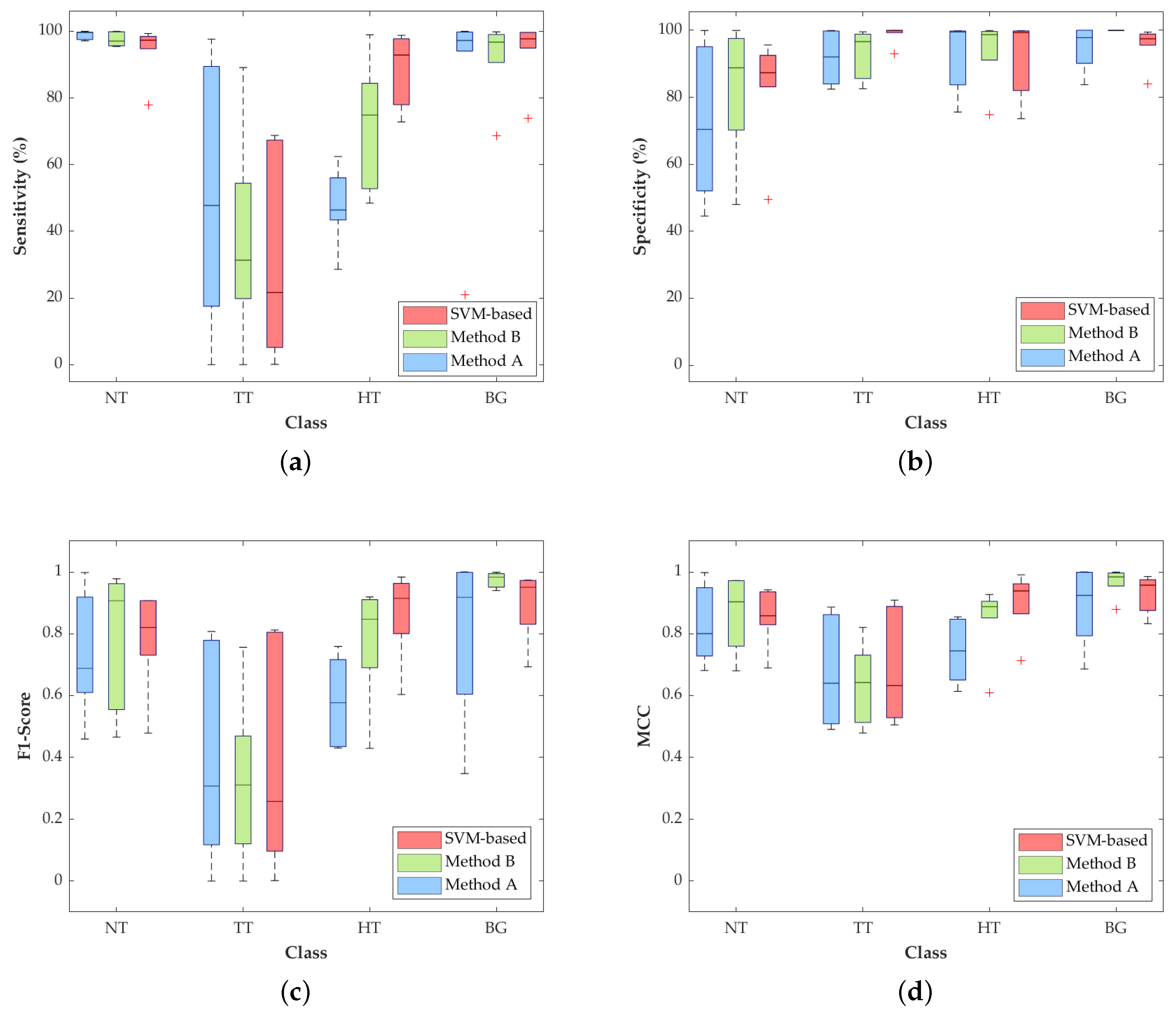
5.2. Comparison Results

In Method B, for the BG class extraction, our analysis shows that the correlation metric is the best option to improve accuracy, and for the tissue classification, the Mahalanobis metric is selected for better performance. Hence, Method A with the correlation metric and Method B with correlation/Mahalanobis metrics are compared to the SVM-based approach. The six test HS images (P008-01, P008-02, P012-01, P012-02, P015-01, and P020-01) are used to evaluate both proposed methodologies against the machine learning approach by a leave-one-patient-out cross-validation. On average, Method A provides an overall accuracy of 67.2 ± 11.5%, while Method B achieves 76.1 ± 12.4%. These results are lower than the accuracy obtained by the SVM-based approach (79.2 ± 15.6%). However, as can be seen in Figure 6, the classification performance obtained with other metrics for each independent class presents some improvements.

The most relevant result for this particular application is the increment in the TT class sensitivity (Figure 6a) with respect to the SVM-based method. Method A and Method B achieve a median sensitivity of 47.8% and 31.3%, respectively, which represent an increase of 26.2% and 9.7% with respect to the result obtained with the SVM approach (21.6%). In addition, the median sensitivity of the NT class is quite constant among the three approaches, being higher than 97% and reaching 99.7% in Method A. On the contrary, the HT class is penalized in Methods A and B, decreasing the median sensitivity result to 46.5% and 18%, respectively, compared to the SVM performance (92.9%). Nonetheless, in this particular application, the accurate identification and differentiation of the NT and TT classes are more important than the identification of the hypervascularized tissue that can be distinguished by the naked eye, or can be identified with an image processing algorithm based on the morphological properties of the blood vessels.

With respect to the specificity results (Figure 6b), all the values for the three proposed methods are quite similar, except for the NT and TT classes, where there are some slight differences among the studied methods. In the NT class, Method A drops its median specificity value to 70.4%, while Method B and SVM scheme reach 88.8% and 87.3%, respectively. The specificity of the TT class is also slightly decreased in the two proposed methods, showing higher interquartile ranges (IQR) than the SVM-based approach, but with median values higher than 92%.

Regarding the F1-score results, Figure 6c shows that, in the TT class, Methods A and B improve the median values by 30.7% and 31%, respectively, compared to the result obtained by the SVM-based approach (25.7%). For the NT and BG classes, Method B obtains the best median results of 90.7% and 98.3%. In contrast, the SVM-based approach reaches the best result in the HT class (91.5%), which is consistent with the results obtained for the sensitivity metric.

Finally, Figure 6d shows the normalized MCC results, which take into account the unbalanced dataset. In these results, the median values of the TT class are quite similar (~66%) among the three methods, while the median of the NT class in Method B reaches the best result of 90.4%. On the contrary, the median of the HT class is reduced in Methods A and B by ~19% and ~5%, respectively, with respect to the SVM-based approach.

The qualitative results represented as classification maps are shown in Figure 7 for Methods A and B and the SVM-based approach. These maps allow evaluating the results obtained in the classification of the all the HS images, including the non-labeled pixels. Figure 7a shows the synthetic RGB images with the tumor area marked by a yellow line, while Figure 7b–d presents the classification maps obtained with the SVM-based approach, Method A and Method B, respectively. In these classification results, the proposed methods improve the labeling of the pixels in the tumor area with respect to the SVM-based approach. However, the proposed methodologies present more false positives in the non-tumor areas. Regarding the other tissue classes, the qualitative results are quite similar, except for the BG class, where Method B shows an accurate identification of the parenchymal area (exposed brain surface) in images P008-01, P008-02, and P012-02. Moreover, by these results, we observe that the low classification performance found in the quantitative results of the HT class in Method A (see Figure 6) is due to the misclassifications between the BG and HT classes in images P008-02 and P015-01, where the main blood vessels are identified as background. This phenomenon does not occur in Method B, where, in general, the hypervascularized areas are well identified.

Regarding the comparison of the execution time among the three methods, Figure 8 shows the average time obtained for the six test HS images. In order to better compare the results, a logarithmic scale is used. This execution time-cost involves both the training and classification for the SVM-based approach and the complete execution of both proposed methods in Figure 2 and Figure 3. These results were computed by using MATLAB^® on an Intel i7-4790K with a working frequency of 4.00 GHz and a RAM memory of 8 GB. The SVM-based approach requires almost four hours to train and perform a classification of one HS image. However, the proposed methods based on the EBEAE algorithm only require an average of ~30 s to train and classify the datasets, achieving similar accuracy results as discussed in the previous paragraphs. In summary, the proposed Methods A and B offer speedup factors of ~459× and ~429×, respectively, compared to the SVM-based approach.

The results obtained in this preliminary study were compared with other works that employed the same database for classification purposes. In [27], five in vivo brain surface HS images with confirmed grade IV glioblastoma tumor were used for brain cancer detection. The SVM algorithm was employed using an intra-patient methodology for evaluating the supervised classifier. This research obtained specificity and sensitivity results higher than 99% for the TT class. However, due to the intra-patient methodology, where the data from the same patient were employed for both training and test, the results were highly optimistic, without taking into account the intra-patient variability of the spectral data. In [28], the authors presented the results obtained with different deep-learning techniques using the in vivo human brain cancer HS dataset employed in this work and evaluated eight HS images using a leave-one-patient-out cross-validation methodology. The sensitivity obtained for the NT and TT classes was 90% and 42%, respectively. Furthermore, the deep-learning results were compared with a linear SVM-based classifier that obtained a sensitivity for the NT and TT classes of 95% and 26%, respectively. However, our results cannot be directly compared to these previous studies, since the testing HS images in the dataset were not the same. In any case, future works with new HS datasets will perform a large comparison among different classification approaches for this particular case of in vivo brain cancer detection using HSI.

6. Conclusions

In this work, we proposed two methods based on a BLU algorithm (EBEAE) to classify intraoperative HS images of in vivo brain tissue, and we compared the results with a machine learning classification method based on a supervised SVM strategy. The main contribution of this paper is achieving a competitive classification performance with respect to the SVM strategy at the lowest computational time cost. One important feature of our proposal is that both Methods A and B require roughly the same computational cost, but we observe, as the advantages of Method B, less variability in the classification performance. Furthermore, as originally intended, Method B is more accurate in identifying the BG class (F1-score and MCC metric), and both Methods A and B improve the sensitivity and F1-score in detecting the TT class compared to the SVM-based approach.

In this study, we were able to achieve speedup factors of ~459× and ~429× by using the proposed methods with respect to the SVM-based approach, while keeping constant and even slightly improving the classification metrics. Note that in Method A, the training stage by using the ground-truth datasets is equivalent to extracting the characteristic end-members per class, and in Method B, we add the segmentation of the background class. Meanwhile, the labeling of the pixels in the HS images is equivalent to computing the minimum distance to the classes’ sets. Both processes are significantly less complex than the training and labeling steps of the SVM-based classifier. Meanwhile, the accuracy results could not be significantly improved due to the intrinsic variability in the intraoperative HS images.

For this particular application, reducing the computational time could allow using the spectral data from the current patient to obtain personalized classification results. This particular information could be combined with previous patient datasets to develop a classification model that takes into account inter-patient and intra-patient spectral variability. Moreover, the massive parallelization capabilities of the proposed BLU methods, together with the use of the so-called snapshot HS cameras (cameras that are able to capture spectral and spatial information in one single shot) that provide real-time HSI, could achieve classification results in real time during clinical procedures, improving the outcomes of the surgery and, hence, the patient outcomes and quality of life.

One of the main limitations of this preliminary study is the reduced number of patients included in the HS brain cancer database for a better generalization of the classification results. This lack of data was produced due to the challenges of obtaining good-quality HS images during surgical procedures. For this reason, in future works, we will include more patients in the HS database in order to further validate the proposed methodology. Furthermore, the inclusion of morphological post-processing methods will be explored to reduce the misclassifications found in the qualitative classification results. Especially the false positives of the tumor class could be reduced if the method is combined with spatial filtering algorithms.

Moreover, further research will be carried out to reduce the processing time of the proposed methodologies by using specific hardware accelerators, such as GPUs (Graphic Processing Units) or FPGAs (field-programmable gate arrays), exploiting the parallelism of these platforms. As stated before, the algorithm acceleration will assist neurosurgeons to identify the tumor area and its boundaries during the surgical procedure, reaching real-time performance.

References

- Vashpanov, Y.; Heo, G.; Kim, Y.; Venkel, T.; Son, J.Y. Detecting Green Mold Pathogens on Lemons Using Hyperspectral Images. Appl. Sci. 2020, 10, 1209. [Google Scholar] [CrossRef]
- Khan, M.J.; Khan, H.S.; Yousaf, A.; Khurshid, K.; Abbas, A. Modern Trends in Hyperspectral Image Analysis: A Review. IEEE Access 2018, 6, 14118–14129. [Google Scholar] [CrossRef]
- Lei, T.; Sun, D.W. Developments of nondestructive techniques for evaluating quality attributes of cheeses: A review. Trends Food Sci. Technol. 2019, 88, 527–542. [Google Scholar] [CrossRef]
- Shimoni, M.; Haelterman, R.; Perneel, C. Hypersectral Imaging for Military and Security Applications: Combining Myriad Processing and Sensing Techniques. IEEE Geosci. Remote Sens. Mag. 2019, 7, 101–117. [Google Scholar] [CrossRef]
- Sudharsan, S.; Hemalatha, R.; Radha, S. A Survey on Hyperspectral Imaging for Mineral Exploration using Machine Learning Algorithms. In Proceedings of the 2019 International Conference on Wireless Communications Signal Processing and Networking (WiSPNET), Chennai, India, 21–23 March 2019; pp. 206–212. [Google Scholar]
- Manni, F.; van der Sommen, F.; Zinger, S.; Shan, C.; Holthuizen, R.; Lai, M.; Bustrom, G.; Hoveling, R.J.; Edstrom, E.; Elmi-Terander, A.; et al. Hyperspectral Imaging for Skin Feature Detection: Advances in Markerless Tracking for Spine Surgery. Appl. Sci. 2020, 10, 4078. [Google Scholar] [CrossRef]
- Lu, G.; Fei, B. Medical hyperspectral imaging: A review. J. Biomed. Opt. 2014, 19, 1–24. [Google Scholar] [CrossRef]
- Kamruzzaman, M.; Sun, D.W. Chapter 5-Introduction to Hyperspectral Imaging Technology. In Computer Vision Technology for Food Quality Evaluation, 2nd ed.; Sun, D.W., Ed.; Academic Press: San Diego, CA, USA, 2016; pp. 111–139. [Google Scholar] [CrossRef]
- Keshava, N.; Mustard, J.F. Spectral unmixing. IEEE Signal Process. Mag. 2002, 19, 44–57. [Google Scholar] [CrossRef]
- Gutierrez-Navarro, O.; Campos-Delgado, D.; Arce-Santana, E.; Jo, J.A. Quadratic blind linear unmixing: A graphical user interface for tissue characterization. Comput. Methods Programs Biomed. 2016, 124, 148–160. [Google Scholar] [CrossRef]
- Dobigeon, N.; Altmann, Y.; Brun, N.; Moussaoui, S. Chapter 6-Linear and Nonlinear Unmixing in Hyperspectral Imaging. In Resolving Spectral Mixtures; Ruckebusch, C., Ed.; Data Handling in Science and Technology; Elsevier: Amsterdam, The Netherlands, 2016; Volume 30, pp. 185–224. [Google Scholar] [CrossRef]
- Shao, Y.; Lan, J.; Zhang, Y.; Zou, J. Spectral Unmixing of Hyperspectral Remote Sensing Imagery via Preserving the Intrinsic Structure Invariant. Sensors 2018, 18, 3528. [Google Scholar] [CrossRef]
- Yao, J.; Meng, D.; Zhao, Q.; Cao, W.; Xu, Z. Nonconvex-Sparsity and Nonlocal-Smoothness-Based Blind Hyperspectral Unmixing. IEEE Trans. Image Process. 2019, 28, 2991–3006. [Google Scholar] [CrossRef]
- Prasad, S.; Chanussot, J. Hyperspectral Image Analysis: Advances in Machine Learning and Signal Processing; Springer Nature: Cham, Switzerland, 2020. [Google Scholar] [CrossRef]
- Li, S.; Song, W.; Fang, L.; Chen, Y.; Ghamisi, P.; Benediktsson, J.A. Deep Learning for Hyperspectral Image Classification: An Overview. IEEE Trans. Geosci. Remote Sens. 2019, 57, 6690–6709. [Google Scholar] [CrossRef]
- Paoletti, M.; Haut, J.; Plaza, J.; Plaza, A. Deep learning classifiers for hyperspectral imaging: A review. ISPRS J. Photogramm. Remote Sens. 2019, 158, 279–317. [Google Scholar] [CrossRef]
- Grigoroiu, A.; Yoon, J.; Bohndiek, S.E. Deep learning applied to hyperspectral endoscopy for online spectral classification. Sci. Rep. 2020, 10, 3947. [Google Scholar] [CrossRef] [PubMed]
- James, G.; Witten, D.; Hastie, T.; Tibshirani, R. An Introduction to Statistical Learning; Springer: New York, NY, USA, 2013. [Google Scholar]
- Tharwat, A. Independent component analysis: An introduction. Appl. Comput. Inform. 2018. [Google Scholar] [CrossRef]
- Nathan, M.; Kabatznik, A.S.; Mahmood, A. Hyperspectral imaging for cancer detection and classification. In Proceedings of the 2018 3rd Biennial South African Biomedical Engineering Conference (SAIBMEC), Stellenbosch, South Africa, 4–6 April 2018; pp. 1–4. [Google Scholar]
- Lu, G.; Halig, L.V.; Wang, D.; Qin, X.; Chen, Z.G.; Fei, B. Spectral-spatial classification for noninvasive cancer detection using hyperspectral imaging. J. Biomed. Opt. 2014, 19, 1–18. [Google Scholar] [CrossRef]
- Masood, K.; Rajpoot, N.; Rajpoot, K.; Qureshi, H. Hyperspectral Colon Tissue Classification using Morphological Analysis. In Proceedings of the 2006 International Conference on Emerging Technologies, Peshawar, Pakistan, 13–14 November 2006; pp. 735–741. [Google Scholar]
- Duann, J.R.; Jan, C.I.; Ou-Yang, M.; Lin, C.Y.; Mo, J.F.; Lin, Y.J.; Tsai, M.H.; Chiou, J.C. Separating spectral mixtures in hyperspectral image data using independent component analysis: Validation with oral cancer tissue sections. J. Biomed. Opt. 2013, 18, 1–8. [Google Scholar] [CrossRef]
- Zhang, D.; Wang, P.; Slipchenko, M.N.; Ben-Amotz, D.; Weiner, A.M.; Cheng, J.X. Quantitative Vibrational Imaging by Hyperspectral Stimulated Raman Scattering Microscopy and Multivariate Curve Resolution Analysis. Anal. Chem. 2013, 85, 98–106. [Google Scholar] [CrossRef] [PubMed]
- Lu, G.; Qin, X.; Wang, D.; Chen, Z.G.; Fei, B. Estimation of tissue optical parameters with hyperspectral imaging and spectral unmixing. In Medical Imaging 2015: Biomedical Applications in Molecular, Structural, and Functional Imaging; Gimi, B., Molthen, R.C., Eds.; International Society for Optics and Photonics, SPIE: St. Bellingham, WA, USA, 2015; Volume 9417, pp. 199–205. [Google Scholar] [CrossRef]
- Campos-Delgado, D.U.; Gutierrez-Navarro, O.; Rico-Jimenez, J.J.; Duran-Sierra, E.; Fabelo, H.; Ortega, S.; Callico, G.; Jo, J.A. Extended Blind End-Member and Abundance Extraction for Biomedical Imaging Applications. IEEE Access 2019, 7, 178539–178552. [Google Scholar] [CrossRef]
- Fabelo, H.; Ortega, S.; Ravi, D.; Kiran, B.R.; Sosa, C.; Bulters, D.; Callicó, G.M.; Bulstrode, H.; Szolna, A.; Piñeiro, J.F.; et al. Spatio-spectral classification of hyperspectral images for brain cancer detection during surgical operations. PLoS ONE 2018, 13, e0193721. [Google Scholar] [CrossRef] [PubMed]
- Fabelo, H.; Halicek, M.; Ortega, S.; Shahedi, M.; Szolna, A.; Piñeiro, J.F.; Sosa, C.; O’Shanahan, A.J.; Bisshopp, S.; Espino, C.; et al. Deep Learning-Based Framework for In Vivo Identification of Glioblastoma Tumor using Hyperspectral Images of Human Brain. Sensors 2019, 19, 920. [Google Scholar] [CrossRef] [PubMed]
- Martinez, B.; Leon, R.; Fabelo, H.; Ortega, S.; Piñeiro, J.F.; Szolna, A.; Hernandez, M.; Espino, C.; O’Shanahan, A.J.; Carrera, D.; et al. Most Relevant Spectral Bands Identification for Brain Cancer Detection Using Hyperspectral Imaging. Sensors 2019, 19, 5481. [Google Scholar] [CrossRef] [PubMed]
- Fabelo, H.; Ortega, S.; Lazcano, R.; Madroñal, D.; Callicó, G.M.; Juárez, E.; Salvador, R.; Bulters, D.; Bulstrode, H.; Szolna, A.; et al. An Intraoperative Visualization System Using Hyperspectral Imaging to Aid in Brain Tumor Delineation. Sensors 2018, 18, 430. [Google Scholar] [CrossRef] [PubMed]
- Salvador, R.; Ortega, S.; Madroñal, D.; Fabelo, H.; Lazcano, R.; Marrero, G.; Juárez, E.; Sarmiento, R.; Sanz, C. HELICoiD: Interdisciplinary and Collaborative Project for Real-Time Brain Cancer Detection: Invited Paper. In Proceedings of the Computing Frontiers Conference; Association for Computing Machinery: New York, NY, USA, 2017; pp. 313–318. [Google Scholar] [CrossRef]
- Fabelo, H.; Ortega, S.; Szolna, A.; Bulters, D.; Piñeiro, J.F.; Kabwama, S.; J-O’Shanahan, A.; Bulstrode, H.; Bisshopp, S.; Kiran, B.R.; et al. In Vivo Hyperspectral Human Brain Image Database for Brain Cancer Detection. IEEE Access 2019, 7, 39098–39116. [Google Scholar] [CrossRef]
- Liu, X.; Yang, C. A Kernel Spectral Angle Mapper algorithm for remote sensing image classification. In Proceedings of the 6th International Congress on Image and Signal Processing (CISP), Hangzhou, China, 16–18 December 2013; Volume 2, pp. 814–818. [Google Scholar]
- Gutierrez-Navarro, O.; Campos-Delgado, D.U.; Arce-Santana, E.R.; Mendez, M.O.; Jo, J.A. Blind End-Member and Abundance Extraction for Multispectral Fluorescence Lifetime Imaging Microscopy Data. IEEE J. Biomed. Health Inform. 2014, 18, 606–617. [Google Scholar] [CrossRef]
- Camps-Valls, G.; Bruzzone, L. Kernel-based methods for hyperspectral image classification. IEEE Trans. Geosci. Remote Sens. 2005, 43, 1351–1362. [Google Scholar] [CrossRef]
- Ortega, S.; Fabelo, H.; Camacho, R.; De la Luz Plaza, M.; Callicó, G.M.; Sarmiento, R. Detecting brain tumor in pathological slides using hyperspectral imaging. Biomed. Opt. Express 2018, 9, 818–831. [Google Scholar] [CrossRef]
- Chang, C.C.; Lin, C.J. LIBSVM: A Library for Support Vector Machines. ACM Trans. Intell. Syst. Technol. 2011, 2. [Google Scholar] [CrossRef]
- Bishop, C.M. Pattern Recognition and Machine Learning; Springer: New York, NY, USA, 2006. [Google Scholar]
- Boughorbel, S.; Jarray, F.; El-Anbari, M. Optimal classifier for imbalanced data using Matthews Correlation Coefficient metric. PLoS ONE 2017, 12, e0177678. [Google Scholar] [CrossRef]
- Otsu, N. A threshold selection method from gray-level histograms. IEEE Trans. Syst. Man Cybern. 1979, 9, 62–66. [Google Scholar] [CrossRef]
- Gutierrez-Navarro, O.; Campos-Delgado, D.U.; Arce-Santana, E.R.; Maitland, K.C.; Cheng, S.; Jabbour, J.; Malik, B.; Cuenca, R.; Jo, J.A. Estimation of the number of fluorescent end-members for quantitative analysis of multispectral FLIM data. Opt. Express 2014, 22, 12255–12272. [Google Scholar] [CrossRef]
- Conci, A.; Kubrusly, C. Distance Between Sets—A survey. Adv. Math. Sci. Appl. 2017, 26, 1–18. [Google Scholar]
- Jain, A.K. Data clustering: 50 years beyond K-means. Pattern Recognit. Lett. 2010, 31, 651–666. [Google Scholar] [CrossRef]
© 2020 by the authors. Licensee MDPI, Basel, Switzerland. This article is an open access article distributed under the terms and conditions of the Creative Commons Attribution (CC BY) license (http://creativecommons.org/licenses/by/4.0/).