Analysis on Dynamic Contact Characteristics and Dynamic Stiffness Estimating Method of Single Nut Ball Screw Pair Based on the Whole Rolling Elements Model

Abstract

The purpose of this paper is investigating the characteristics of dynamic contact and dynamic stiffness of the single nut ball screw pair (SNBSP). Then a new sensorless method is proposed to extract the SNBSP dynamic contact stiffness of a mass production CNC machine tool feed system. First of all, the transformation relationship between each coordinate system of SNBSP is established. Secondly, the dynamic model of all ball–raceway contact pairs is established. Based on this, a dynamic contact stiffness model is established. The dynamic contact parameters are obtained by the numerical method. It is found that the influence of screw speed on screw and nut raceway normal force distribution are opposite. This will affect the variations of dynamic contact stiffness. It is also clear that the effect of axial load on dynamic stiffness is significant. Then, an effective method is proposed to estimate the dynamic contact stiffness of a mass production CNC machine tool feed system without any external sensors. The axial force of feed system is estimated by using torque current of servo motor. Current signals can be obtained through FANUC Open CNC API Specifications (FOCAS) library functions, and then dynamic contact stiffness can be calculated through the stiffness model without external sensors. Finally, a feed system dynamic model is built, and the contact model and sensorless stiffness estimating method are verified by experiments in this dynamic system.

1. Introduction

Machining accuracy is a key feature to measure the overall performance of CNC machine tools. Ball screws are widely used in CNC machine tool feed systems because they have great stiffness, small axial clearance, high bearing capacity and low frictional force [1]. Although the ball screws have used in CNC machine tool systems for many years, the contact parameters of the screw nut pair, especially dynamic contact stiffness for keeping the feed system’s positioning accuracy and precision, are still not fully explained.

The contact stiffness of ball screw pair depends on ball and raceway contact state. However, the ball screw pair has complex surfaces, thus internal motion of rolling elements is difficult to directly analyze. Therefore, a lot of numerical analysis methods have been studied to analyze it. A half lead model of double nuts ball screws is built by Hirokazu Shimoda et al. [2], and load distribution properties were analyzed. It was assumed that the normal force of the contact pair in every half lead was the same, and the phenomenon could be found from the computational results that load distribution was uneven with the unit of half a lead. Bertolaso et al. [3] verified the ball screw nut pair’s uneven distribution, through photoelasticity, tag tracking and the FEM numerical method based on the half lead model. However, the models proposed by the above scholars cannot describe the contact state of the whole ball–raceway pairs, and the research on the screw nut is still in the stage of static analysis. Huang et al. [4] introduced the method of medial axis transform (MAT), and analyzed normal force, contact angle and contact stress of contact surface between the ball and the raceway. Lin et al. [5] researched ball screw pair kinematic characteristics by using the Frenet–Serret coordinate system, and proved that a sliding state existed in the screw and nut raceway. At the same time, Lin et al. [6] also proposed three methods to obtain ball screws’ mechanical efficiency. Based on his theory, the optimization design of the ball screw pair mechanical structure was carried out. According to the literature [5], Wei et al. [7] carried out further research, and analyzed the dynamic variation of the contact angle, frictional force and slip angle of the contact surface between the ball and the raceway. However, the above scholars’ ball screw pair dynamic analysis was in view of the assumption that the loading force of all the ball–raceway contact pairs is evenly distributed, which is contrary to the research results of Hirokazu and Bertolaso. Xu [8] investigated friction characteristics. The effect of creep parameters on the ball screw friction and friction distribution were analyzed. Chen [9] researched rolling element bearing, creep in one lap of ball screw nut pair, but he did not analyze all laps of the pairs. The axial, torsional and bending dynamic models of the ball screw were built, and the stiffness, mass and damping matrix of the system were derived [9,10]. Wu et al. [11] established the mathematical model of the axial and torsional stiffness of the ball screw based on the fixed constraint of the ball screw. By using Simulink, a simulation model of CNC machine tool feed system considering the stiffness was established. However, the contact stiffness model of ball screw pair is not accurate because all contact states of ball and raceway are not considered. Moreover, the extraction of dynamic contact stiffness of ball screw pair has not been applied to mass production CNC machine tools.

In view of the above problems, a dynamic contact model of a single nut ball screw pair (SNBSP) was proposed. Dynamic contact characteristics of an SNBSP were analyzed. Then, the stiffness sensorless estimating method of SNBSP was carried out. This paper consists of the following parts: In Section 2, dynamic contact mechanics model of an SNBSP was proposed. In Section 3, the influence of dynamic factors on contact normal force, contact angle and contact stiffness distribution characteristics of contact pairs are analyzed. In Section 4, a stiffness sensorless estimating method of SNBSP was proposed. An experiment is carried out by which the model is verified. Finally, Section 5 contains the conclusions.

2. Dynamic Contact Model of SNBSP

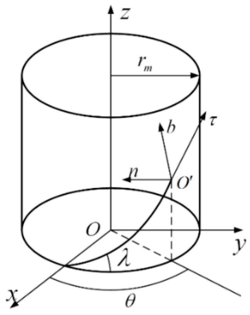
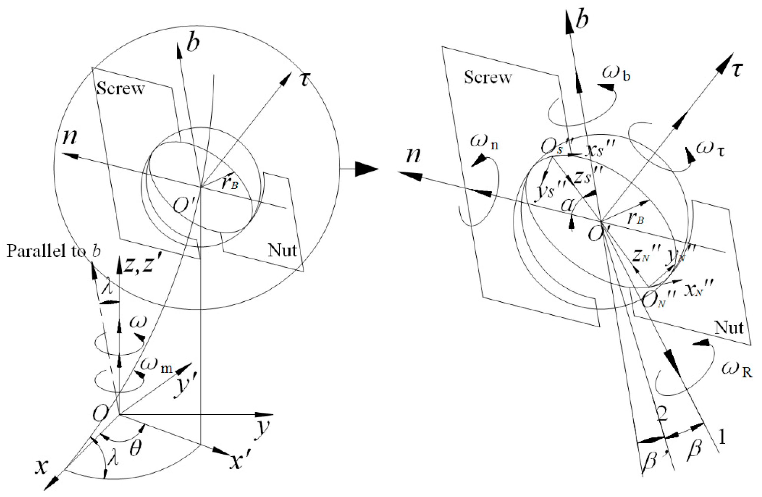
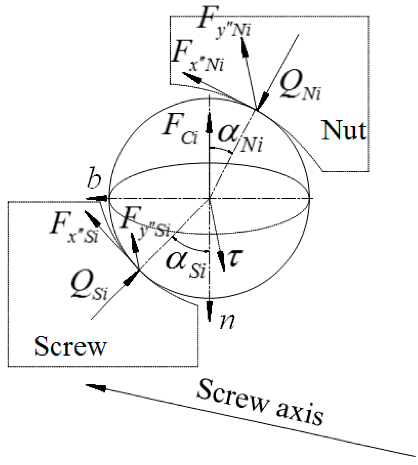
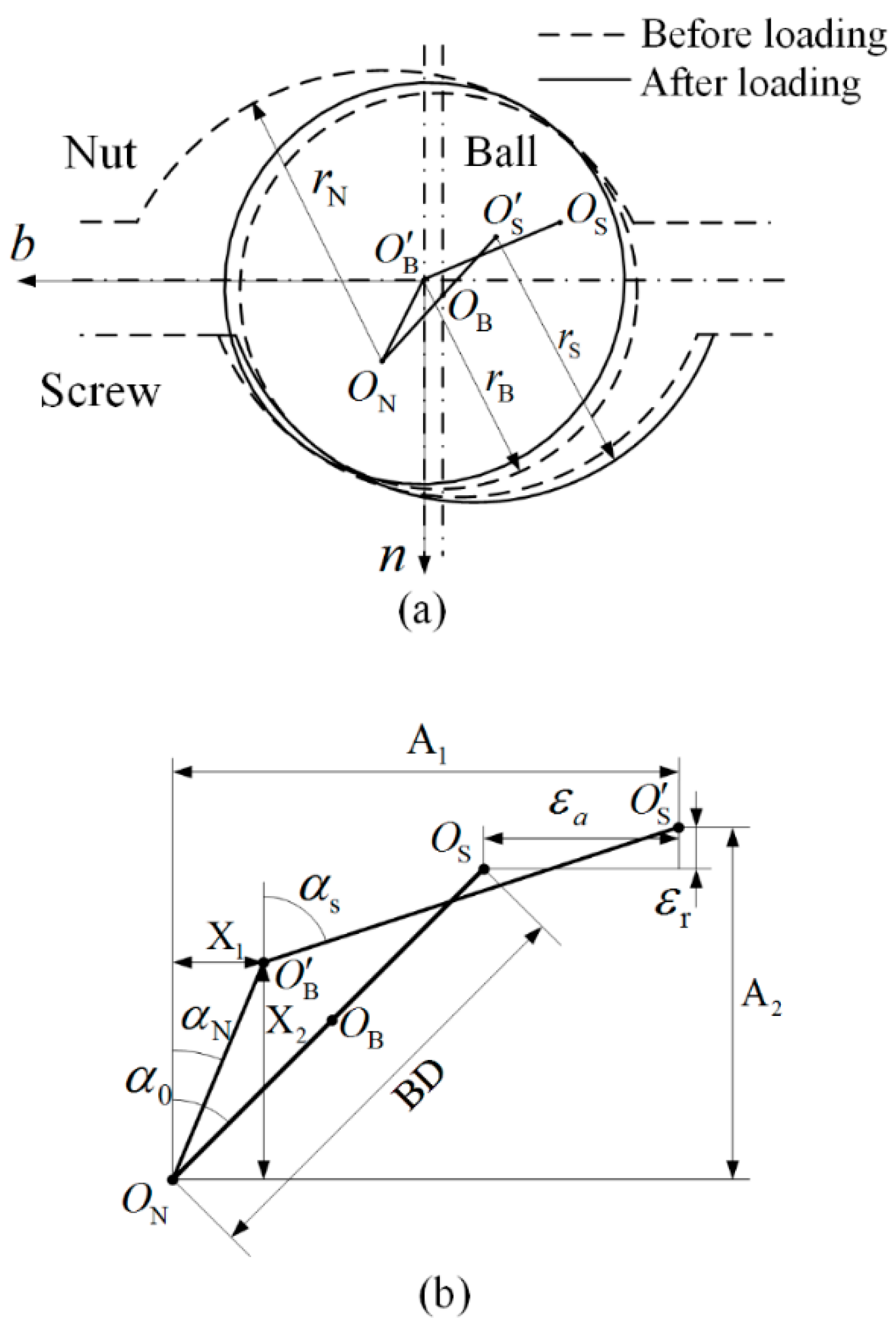
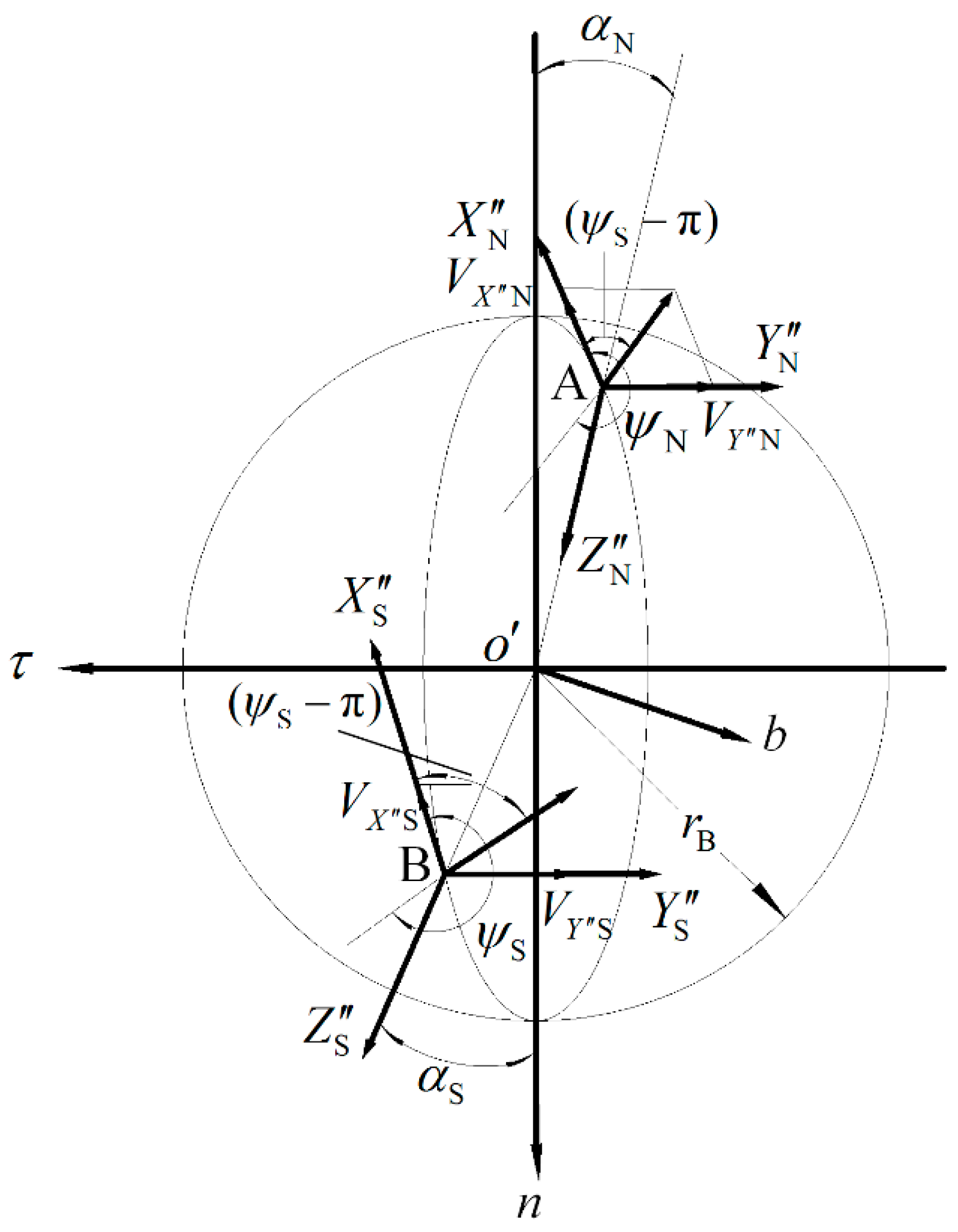
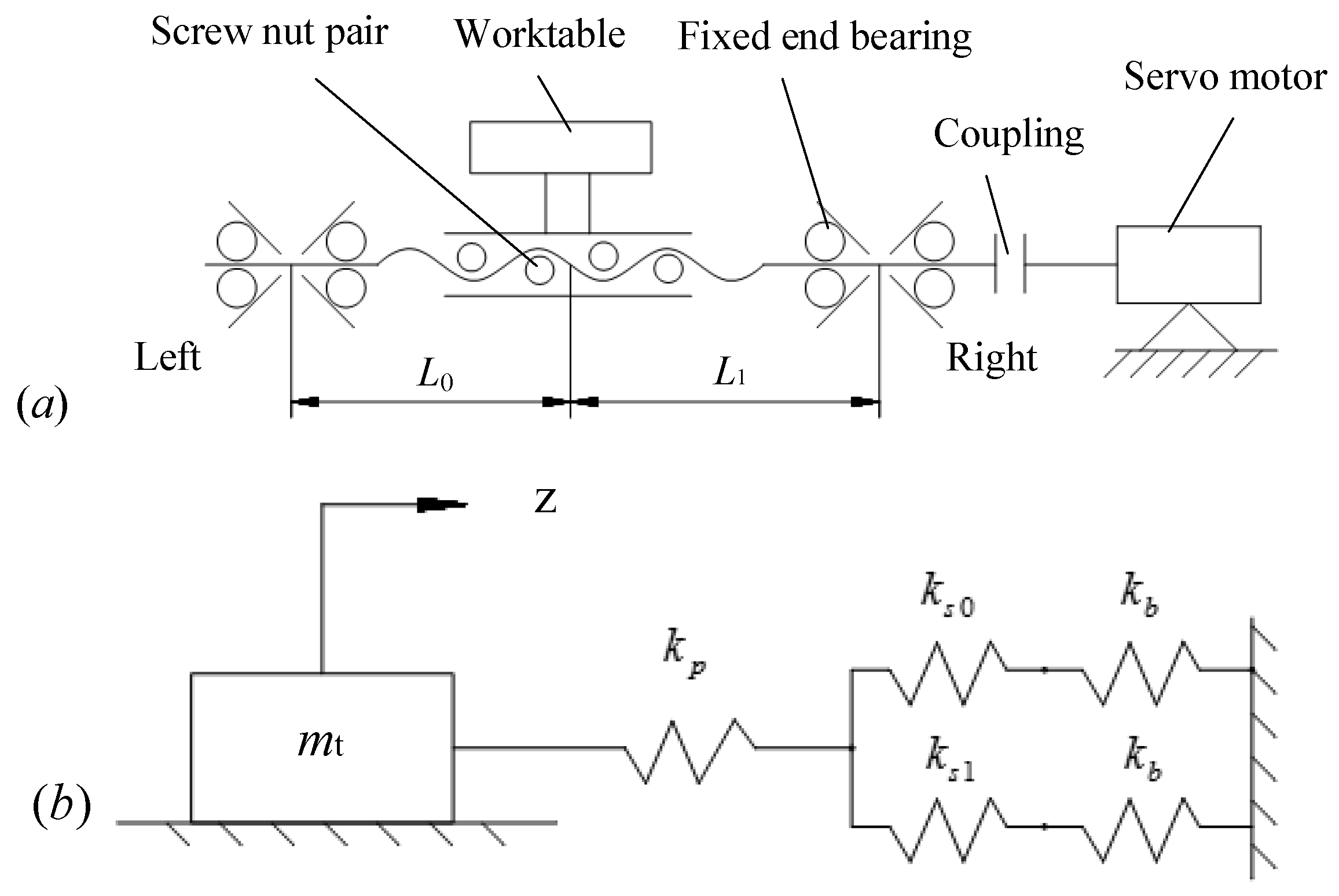
2.1. Setting and Transformation of the Coordinate System

For researching the movement and contact characteristics of a screw and nut conveniently, three coordinate systems are introduced in this paper.

Rotating coordinate system $Oxyz$: The direction of z axis is consistent with that of screw, and its rotating speed will be the same as the screw speed (Figure 1).

Local coordinate system $O^{\prime }\tau nb$: In order to describe the contact pair during movement, the Frenet frame is selected and the Cartesian coordinate system is carried out to establish CS$O^{\prime }\tau nb$. The center of the coordinate is the ball center. The direction of the $n$ axis is consistent with the screw radial direction at the $O^{\prime }$ point. The tangent direction of the helix at point $O^{\prime }$ is the $\tau$ axis. The direction of the $b$ axis is determined by the $\tau$ axis and $n$ axis through the right-hand rule (Figure 1).

Contact coordinate system $O_{\varsigma }^{″}{x}_{\varsigma }^{″}{y}_{\varsigma }^{″}{z}_{\varsigma }^{″}$ is established (Figure 2). When $\varsigma =S$, it denotes the contact area between the ball and the screw raceway. When $\varsigma =N$, it denotes the contact area between the ball and the nut raceway. Take CS$O_S^{″}{x}_S^{″}{y}_S^{″}{z}_S^{″}$ as an example—$O_S^{″}$ denotes the contact point between the ball and the screw. The direction of the $x_S^{″}$ axis coincides with the tangent direction, which crosses the $O_S^{″}$ point, of the contact curve between the rolling element and the lead screw. The direction of the $z_S^{″}$ axis coincides with the normal direction of the contact curve crossing the $O_S^{″}$ point between the rolling element and the lead screw. The $y_S^{″}$ axis direction is determined by the right-hand rule [12].

The transformation relationship between the rotating coordinate system CS$Oxyz$ and the local coordinate system CS$O^{\prime }\tau nb$ can be obtained by the following formula:

$$\begin{array}{c}\left\{\begin{array}{l}x\\ y\\ z\\ 1\end{array}\right\}=Trans\left(r_m\cos \theta ,r_m\sin \theta ,r_m\theta \tan \lambda \right)Rot\left(z,\theta +\frac{\pi }{2}\right)Rot\left(y,-\lambda \right)\left\{\begin{array}{l}\tau \\ n\\ b\\ 1\end{array}\right\}\\ =\left[\begin{array}{cccc}-\cos \lambda \sin \theta & -\cos \theta & \sin \theta \sin \lambda & r_m\cos \theta \\ \cos \lambda \cos \theta & -\sin \theta & -\sin \lambda \cos \theta & r_m\sin \theta \\ \sin \lambda & 0& \cos \lambda & r_m\theta \tan \lambda \\ 0& 0& 0& 1\end{array}\right]\left\{\begin{array}{l}\tau \\ n\\ b\\ 1\end{array}\right\}\end{array}$$

(1)

where $\lambda$ denotes the lead angle of the ball screw, $r_m$ denotes the screw pitch radius, and $\theta$ denotes the position angle of the ball.

Let the transformation matrix between CS$Oxyz$ and CS$O^{\prime }\tau nb$ be $T_{0-1}$. Equation (1) can be written as follows,

$${\left\{x,y,z,1\right\}}^T=T_{0-1}{\left\{\tau ,n,b,1\right\}}^T$$

(2)

The relationship between CS$O^{\prime }\tau nb$ and CS$O_{\varsigma }^{″}{x}_{\varsigma }^{″}{y}_{\varsigma }^{″}{z}_{\varsigma }^{″}$ can be represented as follows,

$${\left\{\tau ,n,b,1\right\}}^T=T_{1-2\varsigma }{\left\{x_{\varsigma }^{″},y_{\varsigma }^{″},z_{\varsigma }^{″},1\right\}}^T$$

(3)

where $T_{1-2\varsigma }$ denotes the transformation matrix.

$$T_{1-2\varsigma }=\left[\begin{array}{cccc}0& 1& 0& 0\\ -\sin {\alpha }_{\varsigma }& 0& \cos {\alpha }_{\varsigma }& \eta r_B\cos {\alpha }_{\varsigma }\\ \cos {\alpha }_{\varsigma }& 0& \sin {\alpha }_{\varsigma }& \eta r_B\sin {\alpha }_{\varsigma }\\ 0& 0& 0& 1\end{array}\right]$$

(4)

where, when $\varsigma =S$, $\eta =1$. When $\varsigma =N$, $\eta =-1$. ${\alpha }_{\varsigma }$ denotes the contact angle between the ball and the screw (or nut) raceway.

The transformation relation between CS$Oxyz$ and CS$O_{\varsigma }^{″}{x}_{\varsigma }^{″}{y}_{\varsigma }^{″}{z}_{\varsigma }^{″}$ can be derived from Equations (2) and (3).

$${\left\{x,y,z,1\right\}}^T=T_{0-2\varsigma }{\left\{x_{\varsigma }^{″},y_{\varsigma }^{″},z_{\varsigma }^{″},1\right\}}^T$$

(5)

where

$$T_{0-2\varsigma }=T_{0-1}{T}_{1-2\varsigma }$$

(6)

Here, set the tiny position and the orientation of SNBSP in CS$Oxyz$ is $\Delta P_0$, and it in CS$O_{\varsigma }^{″}{x}_{\varsigma }^{″}{y}_{\varsigma }^{″}{z}_{\varsigma }^{″}$ is $\Delta P_{2\varsigma }$. Then, $\Delta P_0$ and $\Delta P_{2\varsigma }$ can be express as follows [13],

$$\Delta {\mathit{P}}_0=\left[\begin{array}{cccc}1& -{\varphi }_z& {\varphi }_y& dx\\ {\varphi }_z& 1& -{\varphi }_x& dy\\ -{\varphi }_y& {\varphi }_x& 1& dz\\ 0& 0& 0& 1\end{array}\right]$$

(7)

$$\Delta {\mathit{P}}_{2\varsigma }=\left[\begin{array}{cccc}1& -{\varphi }_{z_{2\varsigma }}& {\varphi }_{y_{2\varsigma }}& d{x}_{2\varsigma }\\ {\varphi }_{z_{2\varsigma }}& 1& -{\varphi }_{x_{2\varsigma }}& d{y}_{2\varsigma }\\ -{\varphi }_{y_{2\varsigma }}& {\varphi }_{x_{2\varsigma }}& 1& d{z}_{2\varsigma }\\ 0& 0& 0& 1\end{array}\right]$$

(8)

The following formula can be obtained through differential transformation theory

$$dT=\left[\Delta {\mathit{P}}_0-\mathit{I}\right]T_{0-2\varsigma }=T_{0-2\varsigma }\left[\Delta {\mathit{P}}_{2\varsigma }-\mathit{I}\right]$$

(9)

Suppose the differential transform operators, respectively

$${\Delta }_0=\Delta {\mathit{P}}_0-\mathit{I}$$

(10)

$${\Delta }_{2\varsigma }=\Delta {\mathit{P}}_{2\varsigma }-\mathit{I}$$

(11)

Put Equation (10) and Equation (11) into Equation (9), and transform it; ${\Delta }_{2\varsigma }$ can be represented by

$${\Delta }_{2\varsigma }=T_{0-2\varsigma }^{-1}{\Delta }_0{T}_{0-2\varsigma }^{}$$

(12)

The right side of the Equation (12) is expanded and the result is simplified. It is clear through analyzing the characteristics of SNBSP that the tiny displacements in the six directions should be investigated in CS$Oxyz$, but only three tiny translation $x_{2\varsigma },y_{2\varsigma }$ and $z_{2\varsigma }$ in CS$O_{\varsigma }^{″}{x}_{\varsigma }^{″}{y}_{\varsigma }^{″}{z}_{\varsigma }^{″}$. Therefore, Equation (12) can be represented as

$${\left\{\mathrm{d}{x}_{2S}\mathrm{d}{y}_{2S}\mathrm{d}{z}_{2S}\mathrm{d}{x}_{2N}\mathrm{d}{y}_{2N}\mathrm{d}{z}_{2N}\right\}}^{\mathrm{T}}=\left[\begin{array}{l}T{\mathit{D}}_{2S-0}\\ T{\mathit{D}}_{2N-0}\end{array}\right]{\left\{\mathrm{d}x\mathrm{d}y\mathrm{d}z{\varphi }_x{\varphi }_y{\varphi }_z\right\}}^{\mathrm{T}}$$

(13)

where $T{\mathit{D}}_{2\varsigma -0}$ denotes the homogeneous coordinate differential transformation matrix of CS$O_{\varsigma }^{″}{x}_{\varsigma }^{″}{y}_{\varsigma }^{″}{z}_{\varsigma }^{″}$ and CS$Oxyz$

$$T{\mathit{D}}_{2\varsigma -0}=\left[\begin{array}{cccccc}\sin {\alpha }_{\varsigma }\cos \theta +\cos {\alpha }_{\varsigma }\sin \lambda \sin \theta & \sin {\alpha }_{\varsigma }\sin \theta -\cos {\alpha }_{\varsigma }\sin \lambda \cos \theta & \cos {\alpha }_{\varsigma }\cos \lambda & {\zeta }_1& {\zeta }_2& {\zeta }_3\\ -\cos \lambda \sin \theta & \cos \lambda \cos \theta & \sin \lambda & {\zeta }_4& {\zeta }_5& {\zeta }_6\\ -\cos {\alpha }_{\varsigma }\cos \theta +\sin {\alpha }_{\varsigma }\sin \lambda \sin \theta & -\cos {\alpha }_{\varsigma }\sin \theta -\sin {\alpha }_{\varsigma }\sin \lambda \cos \theta & \sin {\alpha }_{\varsigma }\cos \lambda & {\zeta }_7& {\zeta }_8& {\zeta }_9\end{array}\right]$$

(14)

where

$$\begin{array}{c}\begin{array}{ll}{\zeta }_1\hfill & =r_m\theta \left[\left(\cos {\alpha }_{\varsigma }\cos \theta -\sin {\alpha }_{\varsigma }\sin \lambda \sin \theta \right)/\cos \lambda -\cos {\alpha }_{\varsigma }\cos \lambda \cos \theta \right]\\ \hfill & +r_m\cos {\alpha }_{\varsigma }\cos \lambda \sin \theta -\eta r_B\cos \lambda \sin \theta \end{array}\\ \begin{array}{ll}{\zeta }_2& =r_m\theta \left[\left(\cos {\alpha }_{\varsigma }\sin \theta +\sin {\alpha }_{\varsigma }\sin \lambda \cos \theta \right)/\cos \lambda -\cos {\alpha }_{\varsigma }\cos \lambda \sin \theta \right]\\ \hfill & -r_m\cos {\alpha }_{\varsigma }\cos \lambda \cos \theta +\eta r_B\cos \lambda \cos \theta \end{array}\\ {\zeta }_3=-r_{m}cos{\alpha }_{\varsigma }\sin \lambda +\eta r_B\sin \lambda \\ {\zeta }_4=r_m\left(\sin \lambda \sin \theta -\theta \sin \lambda \cos \theta \right)+\eta r_B\left(-\sin {\alpha }_{\varsigma }\cos \theta -\cos {\alpha }_{\varsigma }\sin \lambda \sin \theta \right)\\ {\zeta }_5=r_m\left(-\sin \lambda \cos \theta -\theta \sin \lambda \sin \theta \right)+\eta r_B\left(-\sin {\alpha }_{\varsigma }\sin \theta +\cos {\alpha }_{\varsigma }\sin \lambda \cos \theta \right)\\ {\zeta }_6=-\eta r_{B}cos{\alpha }_{\varsigma }\cos \lambda \\ {\zeta }_7=r_m\theta \left[\left(\sin {\alpha }_{\varsigma }\cos \theta +\cos {\alpha }_{\varsigma }\sin \lambda \sin \theta \right)/\cos \lambda -\sin {\alpha }_{\varsigma }\cos \lambda \cos \theta \right]+r_m\sin {\alpha }_{\varsigma }\cos \lambda \sin \theta \\ {\zeta }_8=r_m\theta \left[\left(\sin {\alpha }_{\varsigma }\sin \theta -\cos {\alpha }_{\varsigma }\sin \lambda \cos \theta \right)/\cos \lambda -\sin {\alpha }_{\varsigma }\cos \lambda \sin \theta \right]-r_m\sin {\alpha }_{\varsigma }\cos \lambda \cos \theta \\ {\zeta }_9=-r_m\sin {\alpha }_{\varsigma }\sin \lambda \end{array}$$

(15)

where, when $\varsigma =S$, $\eta =1$. When $\varsigma =N$, $\eta =-1$.

Then, the relationship of homogeneous coordinate differential transformation between the CS$Oxyz$ and the CS$O_{\varsigma }^{″}{x}_{\varsigma }^{″}{y}_{\varsigma }^{″}{z}_{\varsigma }^{″}$ is derived.

$${\left\{\mathrm{d}x\mathrm{d}y\mathrm{d}z{\varphi }_x{\varphi }_y{\varphi }_z\right\}}^{\mathrm{T}}=T{\mathit{D}}_{0-2SN}{\left\{\mathrm{d}{x}_{2S}\mathrm{d}{y}_{2S}\mathrm{d}{z}_{2S}\mathrm{d}{x}_{2N}\mathrm{d}{y}_{2N}\mathrm{d}{z}_{2N}\right\}}^{\mathrm{T}}$$

(16)

where $T{\mathit{D}}_{0-2SN}$ denotes the homogeneous coordinate differential transformation matrix of CS$Oxyz$ and CS$O_{\varsigma }^{″}{x}_{\varsigma }^{″}{y}_{\varsigma }^{″}{z}_{\varsigma }^{″}$.

$$T{\mathit{D}}_{0-2SN}={\left[\begin{array}{l}T{\mathit{D}}_{2S-0}\\ T{\mathit{D}}_{2N-0}\end{array}\right]}^{-1}$$

(17)

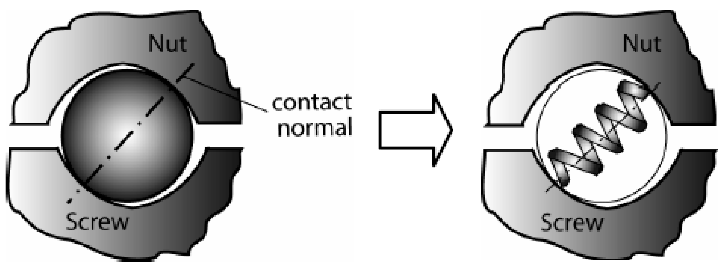
2.2. Dynamic Contact Mechanics Model of SNBSP

In the quasi-static model in which the screw speed is not considered, it is considered that the normal forces and contact angles of the ith ball and the screw and nut raceway are equal, that is,

$${\alpha }_{\mathrm{s}i}={\alpha }_{\mathrm{n}i}\mathrm{and}{Q}_{\mathrm{s}i}=Q_{\mathrm{n}i}$$

(18)

Then the relationship between the axial load and the normal force of contact pair of balls and raceway can be represented as [12],

$$Fa={\displaystyle \sum _{i=1}^z{Q}_{\varsigma i}\sin {\alpha }_{\varsigma i}\cos \lambda }$$

(19)

where $Fa$ denotes the axial force; $Q_{\varsigma i}$ is the normal contact force of the ith contact pair; ${\alpha }_{\varsigma i}$ denotes the contact angle of the ith contact pair. $\varsigma =S,N$. $\lambda$ is the lead angle of screw.

But the rotating screw will drive the balls to generate the angular velocity of the revolution around screw axis and the angular velocity of the ball rotation, respectively, which will make the balls produce outward centrifugal force $F_{\mathrm{C}}$, and produce the transverse frictional force $F_{x^{″}}$ and longitudinal frictional force $F_{y^{″}}$ along the contact surface, which leads to the contact angles of the nut and screw being no longer equal, that is ${\alpha }_{\mathrm{s}i}\ne {\alpha }_{\mathrm{n}i}$. The directions of $F_{x^{″}}$ and $F_{y^{″}}$ are along the $-y_{\varsigma }^{″}$ and $-z_{\varsigma }^{″}$ axes, respectively.

Figure 3 exhibits the force state of the ith ball in CS$O_{\varsigma }^{″}{x}_{\varsigma }^{″}{y}_{\varsigma }^{″}{z}_{\varsigma }^{″}$, and the dynamic balance equation of the ith ball can be obtained from the figure:

$$Q_{\mathrm{S}i}\cos {\alpha }_{\mathrm{S}i}-Q_{\mathrm{N}i}\cos {\alpha }_{\mathrm{N}i}+F_{x^{″}\mathrm{S}i}\sin {\alpha }_{\mathrm{S}i}-F_{x^{″}\mathrm{N}i}\sin {\alpha }_{\mathrm{N}i}+F_{\mathrm{C}i}=0$$

(20a)

$$Q_{\mathrm{S}i}\sin {\alpha }_{\mathrm{S}i}-Q_{\mathrm{N}i}\sin {\alpha }_{\mathrm{N}i}-F_{x^{″}\mathrm{S}i}\cos {\alpha }_{\mathrm{S}i}+F_{x^{″}\mathrm{N}i}\cos {\alpha }_{\mathrm{N}i}=0$$

(20b)

where $F_{x^{″}\varsigma i}$ denotes the transverse friction of the ith contact pair, and $F_{\mathrm{C}i}$ denotes the centrifugal force generated by the rotation of the ith ball. This can be represented as:

$$F_{\mathrm{C}i}=\frac{1}{2}{m}_B{d}_m{\omega }_{mi}^2$$

(21)

where $m_B$ is the ball mass; $d_m$ is the screw helix diameter; and ${\omega }_{mi}$ is the angular velocity of ball revolution along the screw helix of the ith ball.

Then, the relationship between the axial force of the screw nut pair and the loads of the ball and raceway contact pairs can be represented as follows:

$$Fa={\displaystyle \sum _{i=1}^z{Q}_{\varsigma i}\sin {\alpha }_{\varsigma i}\cos \lambda }+{\displaystyle \sum _{i=1}^z{F}_{x^{″}\varsigma i}\cos {\alpha }_{\varsigma i}\cos \lambda }+{\displaystyle \sum _{i=1}^z{F}_{y^{″}\varsigma i}\sin \lambda }$$

(22)

Figure 4 exhibits the load state of the screw $F_{Si}$ and nut $F_{Ni}$ with the ith ball in the screw nut pair. $F_{Si}$ and $F_{Ni}$ can be represented as follows:

$$\begin{array}{ll}{F}_{\varsigma i}\hfill & =Fa-{\displaystyle \sum _{j=1}^{i-1}{Q}_{\varsigma j}\sin {\alpha }_{\varsigma j}\cos \lambda }-{\displaystyle \sum _{j=1}^{i-1}{F}_{x^{″}\varsigma j}\cos {\alpha }_{\varsigma j}\cos \lambda -{\displaystyle \sum _{j=1}^{i-1}{F}_{y^{″}\varsigma j}sin\lambda }}\\ \hfill & ={\displaystyle \sum _{j=i}^z{Q}_{\varsigma j}\sin {\alpha }_{\varsigma j}\cos \lambda }+{\displaystyle \sum _{j=i}^z{F}_{x^{″}\varsigma j}\cos {\alpha }_{\varsigma j}\cos \lambda }+{\displaystyle \sum _{j=i}^z{F}_{y^{″}\varsigma j}sin\lambda }\end{array}$$

(23)

It is known from the deformation relationship between the ith and (i-1)th contact pairs that the deformation increment of the contact pairs of the adjacent balls can be expressed respectively as:

$${\Delta }_{\mathrm{S}i}=\frac{\Delta L{F}_{\mathrm{S}i}}{E_{\mathrm{S}}{A}_{\mathrm{S}}}$$

(24a)

$${\Delta }_{\mathrm{N}i}=\frac{\Delta L{F}_{\mathrm{N}i}}{E_{\mathrm{N}}{A}_{\mathrm{N}}}$$

(24b)

where $\Delta L$ denotes the axial distance between adjacent balls, as shown in Figure 5. $E_S$ and $E_N$ denote the Young modulus of the screw and nut materials, respectively. $A_S$ and $A_N$ denote effective cross-sectional area of the screw and nut, respectively.

$$\Delta L=\frac{d_{\mathrm{m}}\Delta \theta }{2}\tan \lambda$$

(25)

Substituting Equation (23) into Equation (24a), it can be obtained as follows:

$${\Delta }_{\mathrm{S}i}=\frac{d_{\mathrm{m}}\Delta \theta \tan \lambda }{2E_{\mathrm{S}}{A}_{\mathrm{S}}}({\displaystyle \sum _{j=i}^z{Q}_{\mathrm{S}j}\sin {\alpha }_{\mathrm{S}j}\cos \lambda }+{\displaystyle \sum _{j=i}^z{F}_{x^{″}\mathrm{S}j}\cos {\alpha }_{\mathrm{S}j}\cos \lambda }+{\displaystyle \sum _{j=i}^z{F}_{y^{″}\mathrm{S}j}\sin \lambda })$$

(26a)

Substituting Equation (23) into Equation (24b), it can be obtained as follows:

$${\Delta }_{\mathrm{N}i}=\frac{d_{\mathrm{m}}\Delta \theta \tan \lambda }{2E_{\mathrm{N}}{A}_{\mathrm{N}}}({\displaystyle \sum _{j=i}^z{Q}_{\mathrm{N}j}\sin {\alpha }_{\mathrm{N}j}\cos \lambda }+{\displaystyle \sum _{j=i}^z{F}_{x^{″}\mathrm{N}j}\cos {\alpha }_{\mathrm{N}j}\cos \lambda +}{\displaystyle \sum _{j=i}^z{F}_{y^{″}\mathrm{N}j}\sin \lambda })$$

(26b)

According to the deformation coordination relationship, the deformation increment of the ith and the (i-1)th ball screw contact pair and ball nut contact pair can be represented as:

$${\Delta }_{\mathrm{S}i}=({\epsilon }_{\mathrm{S}(i-1)}\sin {\alpha }_{\mathrm{S}(i-1)}-{\epsilon }_{\mathrm{S}i}\sin {\alpha }_{\mathrm{S}i})\cos \lambda$$

(27a)

$${\Delta }_{\mathrm{N}i}=({\epsilon }_{\mathrm{N}(i-1)}\sin {\alpha }_{\mathrm{N}(i-1)}-{\epsilon }_{\mathrm{N}i}\sin {\alpha }_{\mathrm{N}i})\cos \lambda$$

(27b)

Then, according to the Hertz contact theory, there is a relationship between the deformation and the contact force [14,15]:

$${\epsilon }_{\varsigma i}={\kappa }_{\varsigma i}{Q}_{\varsigma i}^{2/3}$$

(28)

$${\kappa }_{\varsigma }=\frac{2K_{\varsigma }(e)}{\pi m_{a\varsigma }}\sqrt[3]{\frac{1}{8}{\left[\frac{3}{2}(\frac{1-{\upsilon }_B^2}{E_B}+\frac{1-{\upsilon }_{\varsigma }^2}{E_{\varsigma }})\right]}^2{\displaystyle \sum {\rho }_{\varsigma B}}}$$

(29)

where ${\upsilon }_B$, ${\upsilon }_S$ and ${\upsilon }_N$ denote the Poisson ratio of the ball, screw and nut, respectively. $E_B,E_S,E_N$ denote the modulus of elasticity of the ball, screw and nut, respectively. ${\displaystyle \sum {\rho }_{SB},{\displaystyle \sum {\rho }_{NB}}}$ denote the summation of principal curvatures of the ball and screw and the ball and nut, respectively. $K(e)$ denotes complete elliptic integral of the first kind, and $m_a$, $m_b$ and $\frac{2K(e)}{\pi m_a}$ can be obtained through the table in reference [16].

Simultaneous Equations (26a) and (27a), and substituting Equation (28) into the equation, it can be obtained as follows:

$$Q_{\mathrm{S}i}^{2/3}\sin {\alpha }_{\mathrm{S}i}={\mathrm{\Gamma }}_{\mathrm{S}i}{Q}_{\mathrm{S}(i-1)}^{2/3}\sin {\alpha }_{\mathrm{S}(i-1)}-{\Psi }_{\mathrm{S}i}{\displaystyle \sum _{j=i}^Z(Q_{\mathrm{S}j}\sin {\alpha }_{\mathrm{S}j}}+F_{x^{″}\mathrm{S}j}\cos {\alpha }_{\mathrm{S}j}+F_{y^{″}\mathrm{S}j}\tan \lambda )\hspace{1em}i=2,3,\cdots ,Z$$

(30a)

In the same way, simultaneous Equations (26b) and (27b), and substituting Equation (28) into the equation, it can be obtained as follow:

$$Q_{\mathrm{N}i}^{2/3}\sin {\alpha }_{\mathrm{N}i}={\mathrm{\Gamma }}_{\mathrm{N}i}{Q}_{\mathrm{N}(i-1)}^{2/3}\sin {\alpha }_{\mathrm{N}(i-1)}-{\Psi }_{\mathrm{N}i}{\displaystyle \sum _{j=i}^Z(Q_{\mathrm{N}j}\sin {\alpha }_{\mathrm{N}j}}+F_{x^{″}\mathrm{N}j}\cos {\alpha }_{\mathrm{N}j}+F_{y^{″}\mathrm{N}j}\tan \lambda )\hspace{1em}i=2,3,\cdots ,Z$$

(30b)

where:

$${\mathrm{\Gamma }}_{\varsigma i}=\frac{{\kappa }_{\varsigma (i-1)}}{{\kappa }_{\varsigma i}},\hspace{1em}{\Psi }_{\varsigma i}=\frac{d_{\mathrm{m}}\Delta \theta \tan \lambda }{2E_{\varsigma }{A}_{\varsigma }{\kappa }_{\varsigma i}}$$

(31)

As a high-speed ball screw nut pair, on the one hand, it mainly bears axial force during operation. On the other hand, the influence of centrifugal force caused by the high-speed rotation of the ball should also be considered. The effect of contact angle, contact force and centrifugal force is considered comprehensively, and the deformation is shown in Figure 6a [17,18]. For analyzing the motion state and deformation of the ball screw nut pair in the motion process, the center of the nut raceway $O_N$ is fixed. As shown in Figure 6b, when the preload is not considered, there is no force between the ball and the screw and nut raceway before the SNBSP under load. So, there is no contact deformation, and the ball center is aligned with the screw and nut raceway curvature center. The internal and external contact angles on both sides of the ball and the raceway are the initial design angle ${\alpha }_0$. When the ball screw is bearing a load, due to internal (screw) and external (nut) contact force and the centrifugal force and the influence of internal and external contact deformation, the ball center moves from the point $O_B$ to $O_B^{\prime }$, the screw raceway curvature center moves from the point $O_S$ to $O_S^{\prime }$, and the contact angles of the ball and screw raceway and nut raceway change from ${\alpha }_0$ to ${\alpha }_{\mathrm{S}}$ and ${\alpha }_{\mathrm{N}}$, respectively.

It can be seen from the geometric relation that,

$$BD=d_{\mathrm{B}}(t_{\mathrm{S}}+t_{\mathrm{N}}-1)$$

(32)

where $t_{\mathrm{S}}$ and $t_{\mathrm{N}}$ are the curvature radius coefficient of the inner and outer raceways, respectively,

$$t_{\varsigma }=r_{\varsigma }/d_B$$

(33)

The geometric analysis of the ith ball after bearing load is as follows:

$$\cos {\alpha }_{\mathrm{N}i}=\frac{X_2}{\left(t_{\mathrm{N}}-0.5\right)d_{\mathrm{B}}+{\epsilon }_{\mathrm{N}i}}$$

(34a)

$$\sin {\alpha }_{\mathrm{N}i}=\frac{X_1}{\left(t_{\mathrm{N}}-0.5\right)d_{\mathrm{B}}+{\epsilon }_{\mathrm{N}i}}$$

(34b)

$$\cos {\alpha }_{\mathrm{S}i}=\frac{A_2-X_2}{\left(t_{\mathrm{S}}-0.5\right)d_{\mathrm{B}}+{\epsilon }_{\mathrm{S}i}}$$

(34c)

$$\sin {\alpha }_{\mathrm{S}i}=\frac{A_1-X_1}{\left(t_{\mathrm{S}}-0.5\right)d_{\mathrm{B}}+{\epsilon }_{\mathrm{S}i}}$$

(34d)

$$A_1=\overline{BD}\sin {\alpha }_0+{\epsilon }_a$$

(34e)

$$A_2=\overline{BD}\cos {\alpha }_0+{\epsilon }_r$$

(34f)

Then, the dynamic contact mechanics model of SNBSP is established which contains Equations (20), (29), (31) and (34a)–(34f).

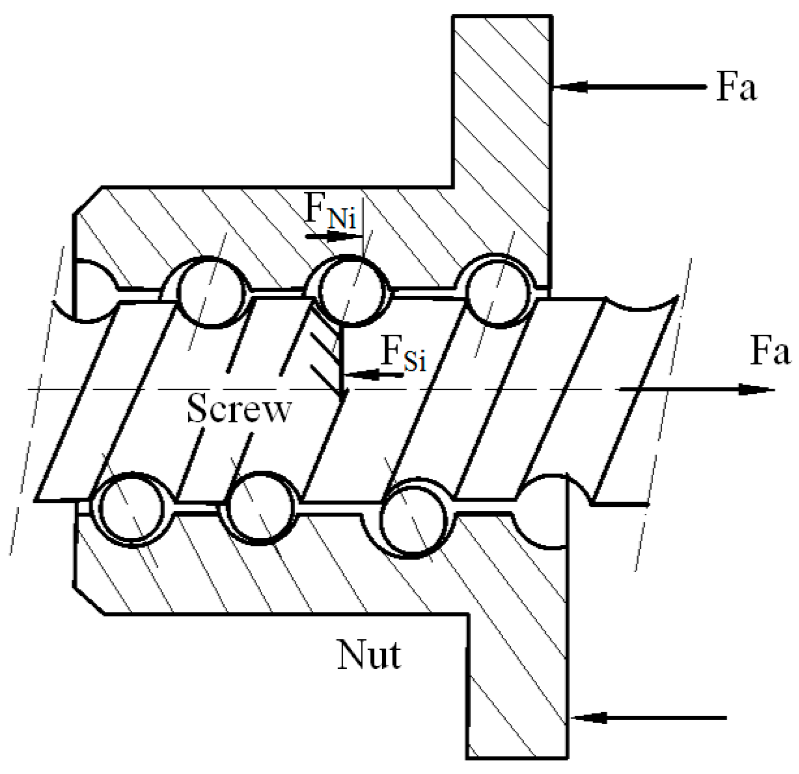
2.3. Calculation of the Frictional Force of SNBSP and Other Related Parameters

2.3.1. The Calculation of Ball and Raceway Contact Pair Frictional Force

As demonstrated in Figure 3, the frictional force between the ball and the screw and nut can be decomposed into two directional components in CS$O_{\varsigma }^{″}{x}_{\varsigma }^{″}{y}_{\varsigma }^{″}{z}_{\varsigma }^{″}$: the $x_{\varsigma }^{″}$ direction (transverse) frictional force and the $y_{\varsigma }^{″}$ direction (longitudinal) frictional force. The formula can be expressed as [7]:

$$F_{x^{″}\varsigma }=a_{\varsigma }{b}_{\varsigma }{\displaystyle {\int }_{-1}^1{\displaystyle {\int }_{-\sqrt{1-{t^{″}}^2}}^{\sqrt{1-{t^{″}}^2}}{\tau }_{x^{″}\varsigma }}d{q}^{″}}d{t}^{″}$$

(35a)

$$F_{y^{″}\varsigma }=a_{\varsigma }{b}_{\varsigma }{\displaystyle {\int }_{-1}^1{\displaystyle {\int }_{-\sqrt{1-{q^{″}}^2}}^{\sqrt{1-{q^{″}}^2}}{\tau }_{y^{″}\varsigma }}d{t}^{″}d{q}^{″}}$$

(35b)

where $a_{\varsigma }$ and $b_{\varsigma }$ denote the semi-major and semi-minor axis of contact ellipse, respectively, the detailed calculation method can be detailed in the reference [16,19]. $q^{″}$ denotes the dimensionless coefficient in the direction of $x_{\varsigma }^{″}$ axis, $q^{″}=x^{″}/a_{\varsigma }$. $t^{″}$ denotes the dimensionless coefficient in the direction of $y_{\varsigma }^{″}$ axis, $t^{″}=y^{″}/b_{\varsigma }$. ${\tau }_{X^{″}\varsigma }$ and ${\tau }_{Y^{″}\varsigma }$ denote the component of the shear stress of the ball and screw or nut in the direction of the $x_{\varsigma }^{″}$ axis and $y_{\varsigma }^{″}$ axis, respectively.

$${\tau }_{x^{″}\varsigma }={\tau }_{\varsigma }\cos ({\psi }_{\varsigma })$$

(36a)

$${\tau }_{y^{″}\varsigma }={\tau }_{\varsigma }\sin ({\psi }_{\varsigma })$$

(36b)

where ${\tau }_{\varsigma }$ denotes the shear stresses of the ball and screw or nut. ${\psi }_{\varsigma }$ denotes the slip angle, which are described in Section 2.3.3.

2.3.2. Calculation of Shear Stress of the Contact Pairs

The shear stress ${\tau }_{\varsigma }$ generated in the contact area between the ball and the screw or ball and nut can be expressed as [4]:

$${\tau }_{\varsigma }=f_{\varsigma }{P}_{\varsigma }$$

(37)

where $f_{\varsigma }$ denotes the frictional coefficient of the contact pair. $P_{\varsigma }$ denotes the Hertz contact pressure on the contact area. The relationship between $P_{\varsigma }$ and $Q_{\varsigma }$ can be represented as:

$$P_{\varsigma }=\frac{3Q_{\varsigma }}{2\pi a_{\varsigma }{b}_{\varsigma }}{\left(1-{q^{″}}^2-{t^{″}}^2\right)}^{1/2}$$

(38)

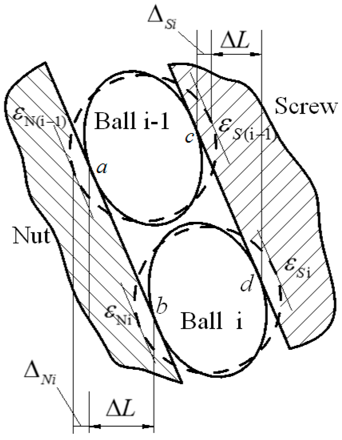
2.3.3. Calculation of the Contact Pairs Slip Angle

The slip angle of the contact pairs reflects the direction of the slip velocity at the contact point in the CS$O_{\varsigma }^{″}{x}_{\varsigma }^{″}{y}_{\varsigma }^{″}{z}_{\varsigma }^{″}$, as shown in Figure 7; it can be expressed as [4]:

$${\psi }_{\varsigma }={\tan }^{-1}\left(\frac{V_{y^{″}\varsigma }}{V_{x^{″}\varsigma }}\right)+\pi$$

(39)

where $V_{x^{″}\varsigma }$ and $V_{y^{″}\varsigma }$ denote the component of the relative slip speed between the contact pair in the direction of the $x_{\varsigma }^{″}$ axis and $y_{\varsigma }^{″}$ axis, respectively. The relationship between the two parameters is as follows [5]:

Relative slip velocity component of the ball screw contact pair:

$$\frac{V_{y^{″}\mathrm{S}}}{V_{x^{″}\mathrm{S}}}=\frac{d\left({\omega }_m-\omega \right)-r_B\left[\left({\omega }_b-\omega \cos \lambda \right)\cos {\alpha }_{\mathrm{S}}-{\omega }_n\sin {\alpha }_{\mathrm{S}}\right]}{r_B\left({\omega }_t-\omega \sin \lambda \right)}$$

(40a)

Relative slip velocity component of the ball nut contact pair:

$$\frac{V_{y^{″}\mathrm{N}}}{V_{x^{″}\mathrm{N}}}=\frac{d{\omega }_m+r_B\left({\omega }_b\cos {\alpha }_{\mathrm{N}}-{\omega }_n\sin {\alpha }_{\mathrm{N}}\right)}{-r_B{\omega }_t}$$

(40b)

where ${\omega }_t,{\omega }_{\mathrm{n}}$ and ${\omega }_b$ denote the component of the angular velocity of the ball rolling in the direction of the t-, n- and b- axis in CS$O^{\prime }\tau nb$, respectively. The calculation process of ${\omega }_t,{\omega }_{\mathrm{n}},{\omega }_b$ and ${\omega }_m$ can be obtained in reference [7], so there is no repeat on it. The direction of each velocity is shown in Figure 2.

2.4. Dynamic Contact Stiffness Model of SNBSP

In the dynamic contact stiffness model, the rolling element is usually regarded as a spring without mass, which is connected along the contact point with the screw and nut raceway (Figure 8).

Stiffness refers to the ability of the material to resist the deformation of external forces. When the ball is in contact with the internal and external raceway, the screw raceway and the nut raceway all have contact deformation. For the ith ball, its normal contact stiffness with the raceway is represented as [20].

$$k_{\varsigma i}=Q_{\varsigma i}^{}/{\epsilon }_{\varsigma i}=K_{\varsigma }^{-1}{Q}_{\varsigma i}^{1/3}$$

(41)

The contact stiffness matrix of the SNBSP can be derived though the transformation relations of CS$Oxyz$, CS$O^{\prime }\tau nb$ and CS$O_{\varsigma }^{″}{x}_{\varsigma }^{″}{y}_{\varsigma }^{″}{z}_{\varsigma }^{″}$. In CS$O^{\prime }\tau nb$, the stiffness of the ith ball with the raceway can be represented as:

$${\mathit{K}}_{\varsigma i}^{″}=\left[\begin{array}{ccc}0& 0& 0\\ 0& 0& 0\\ 0& 0& k_{\varsigma i}\end{array}\right]$$

(42)

where $k_{\varsigma i}$ can be obtained through Equation (41).

Then the contact stiffness between the ith ball and raceway in CS$Oxyz$ can be represented as

$${\mathit{K}}_i=T{\mathit{D}}_{0-2SN}^T\left[\begin{array}{ll}{\mathit{K}}_{Si}^{″}& \\ & {\mathit{K}}_{Ni}^{″}\end{array}\right]T{\mathit{D}}_{0-2SN}^{}$$

(43)

${\mathit{K}}_i$ is the symmetrical matrix, the form of which is expressed as,

$${\mathit{K}}_i=\left[\begin{array}{ccccc}{k}_{i-xx}& & & & \\ k_{i-xy}& k_{i-yy}& & sym& \\ k_{i-xz}& k_{i-yz}& k_{i-zz}& & \\ k_{i-x{\varphi }_x}& k_{i-y{\varphi }_x}& k_{i-z{\varphi }_x}& k_{i-{\varphi }_x{\varphi }_x}& \\ k_{i-x{\varphi }_y}& k_{i-y{\varphi }_y}& k_{i-z{\varphi }_y}& k_{i-{\varphi }_x{\varphi }_y}& k_{i-{\varphi }_y{\varphi }_y}\end{array}\right]$$

(44)

The leading diagonal elements reflect the local variation of contact pairs. Therefore, the concept of local contact stiffness is proposed in this paper. The expression of local contact stiffness in all directions is shown in Equation (45). $K_{i-x},K_{i-y}$ are the local lateral stiffness. $K_{i-z}$ is the local axial stiffness. $K_{i-{\varphi }_x},K_{i-{\varphi }_y}$ are the local oscillating stiffness.

$$K_{i-x}=k_{i-xx}\hspace{1em}{K}_{i-y}=k_{i-yy}\hspace{1em}{K}_{i-z}=k_{i-zz}\hspace{1em}{K}_{i-{\varphi }_x}=k_{i-{\varphi }_x{\varphi }_x}\hspace{1em}{K}_{i-{\varphi }_y}=k_{i-{\varphi }_y{\varphi }_y}$$

(45)

In the ball screw pair, the relationship between each ball and the raceway contact pair is parallel. Therefore, the contact stiffness in all directions in CS$Oxyz$ is represented as:

$$K_x={\displaystyle \sum _{i=1}^n{K}_{i-x}}\hspace{1em}{K}_y={\displaystyle \sum _{i=1}^n{K}_{i-y}}\hspace{1em}{K}_z={\displaystyle \sum _{i=1}^n{K}_{i-z}}\hspace{1em}{K}_{{\varphi }_x}={\displaystyle \sum _{i=1}^n{K}_{i-{\varphi }_x}}\hspace{1em}{K}_{{\varphi }_y}={\displaystyle \sum _{i=1}^n{K}_{i-{\varphi }_y}}$$

(46)

3. Numerical Analysis of Dynamic Contact Characteristics

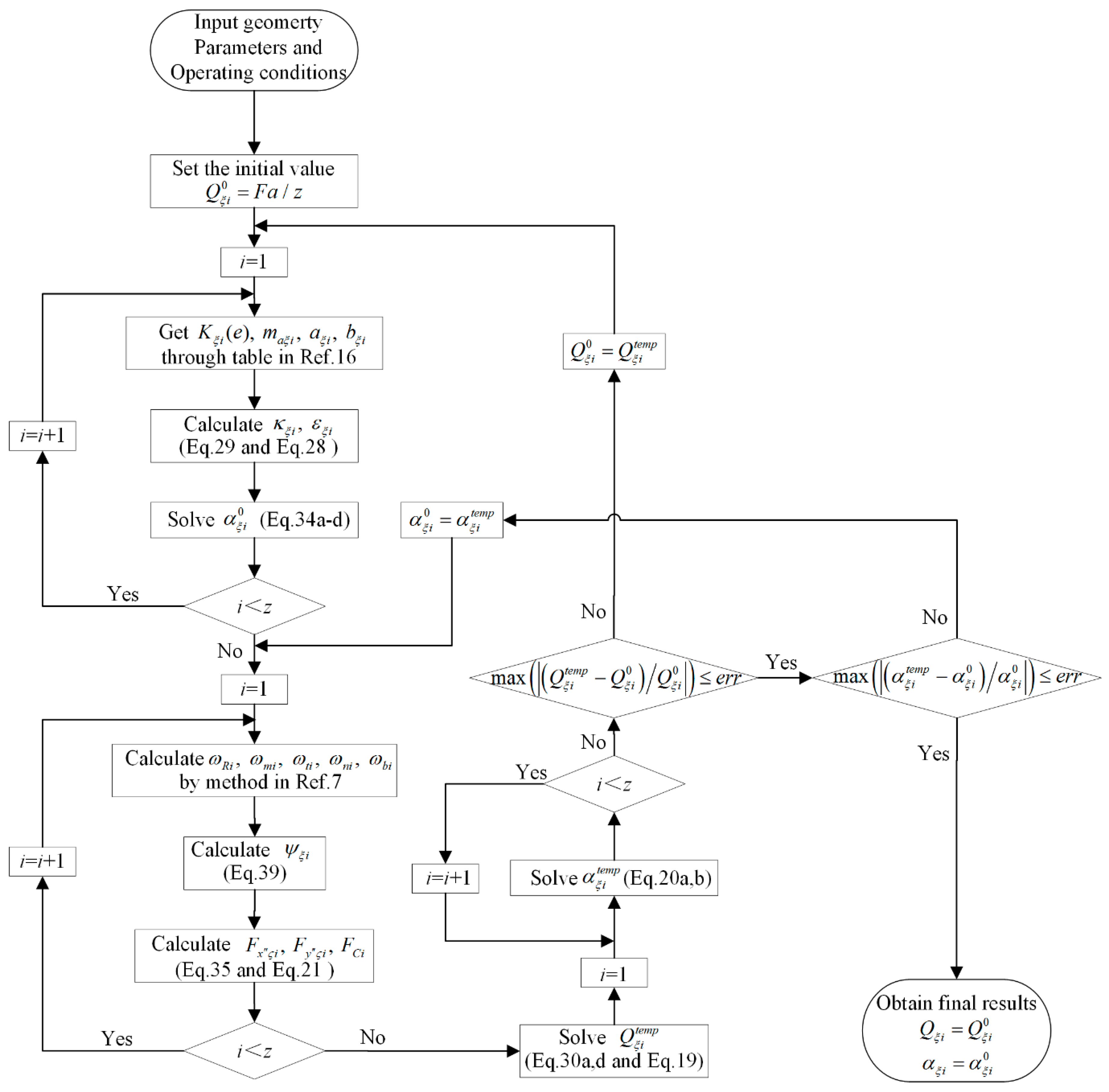
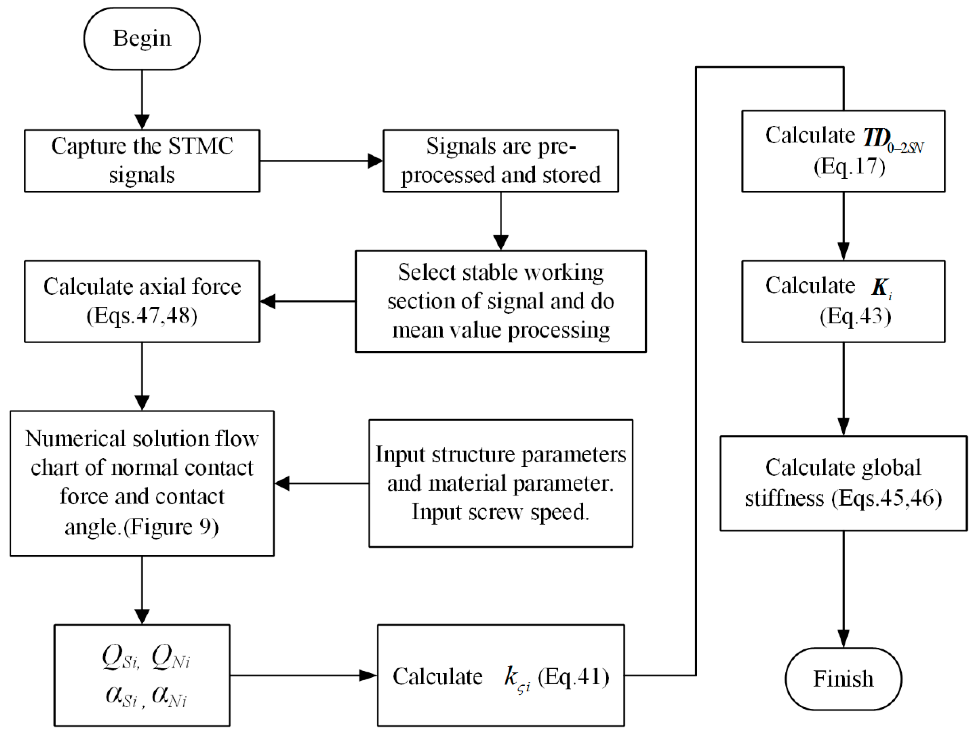
3.1. Flow Chart of Numerical Calculation Method

The flow chart in Figure 9 describes the process of calculating the contact parameters of each contact pair by using the numerical solution based on the dynamic contact mechanics model of SNBSP in this paper.

Table 1. Structure and size parameters of the SNBSP.

Parameter	Value	Unit
Nominal diameter of screw	32	mm
Screw lead	10	mm
Ball diameter	5.95	mm
Raceway curvature ratio	1.07
Number of rolling elements around screw in nut	63
Effective turn numbers of balls	3.5
Nut outer diameter	58	mm
Elastic modulus	210	GPa
Poisson ratio	0.3

is the structure and size parameters of SNBSP. The parameters are taken into each equation, and the results of each dynamic contact parameter can be solved by iterative operation.

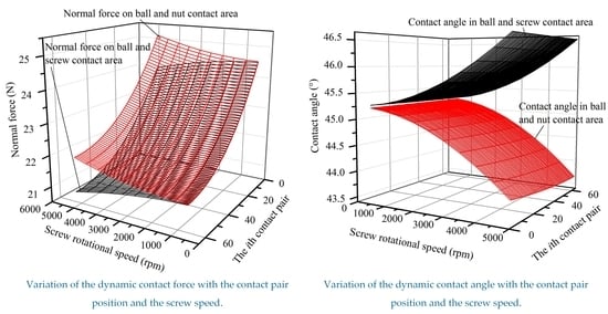
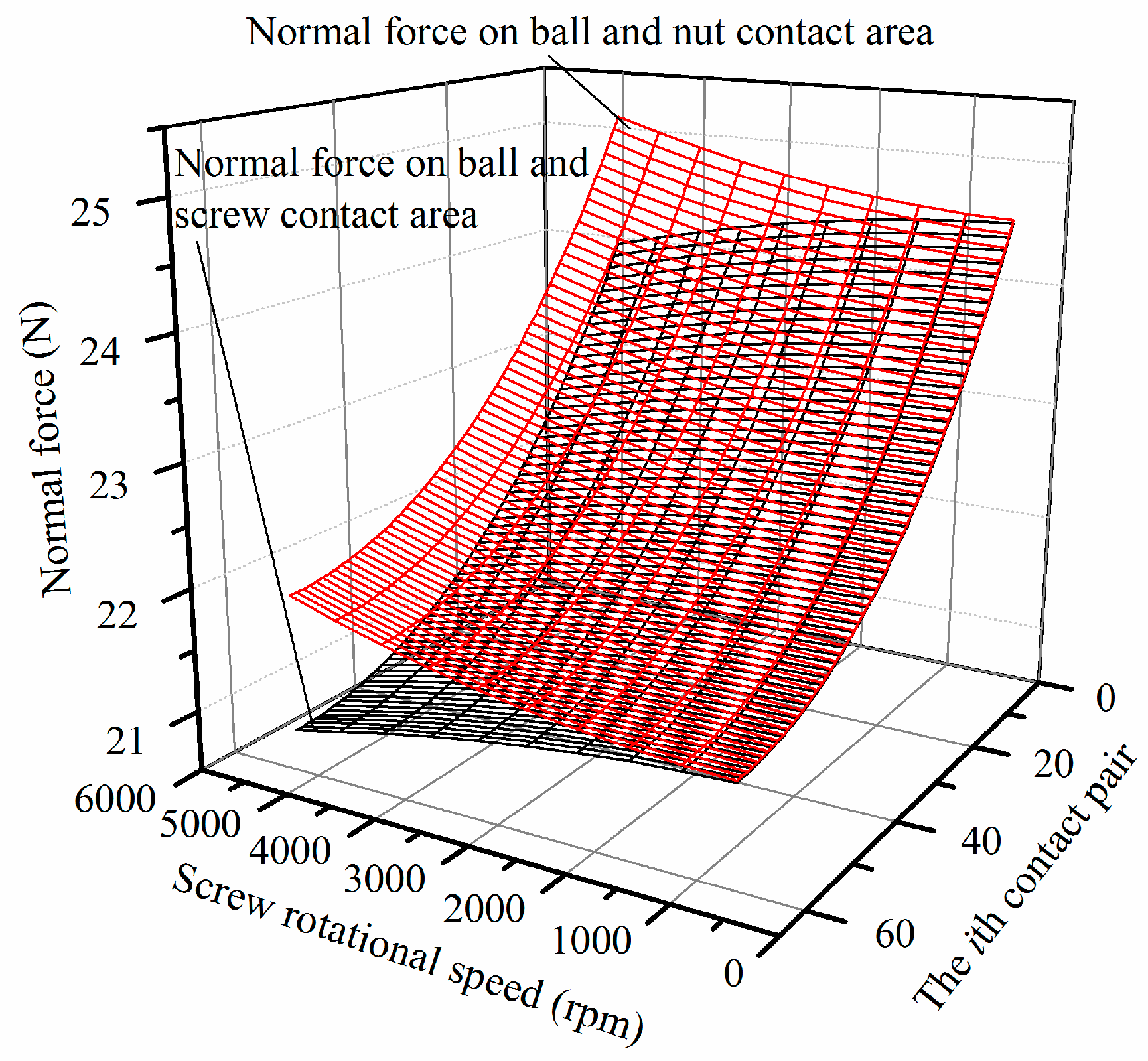
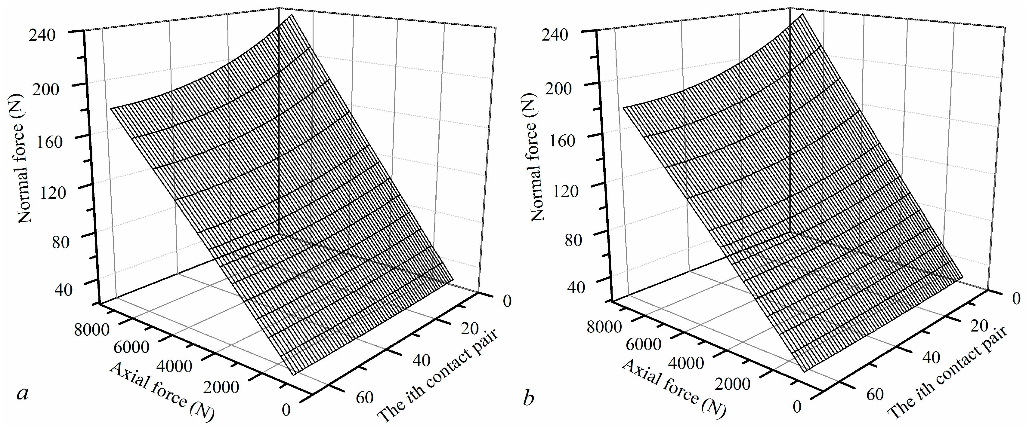
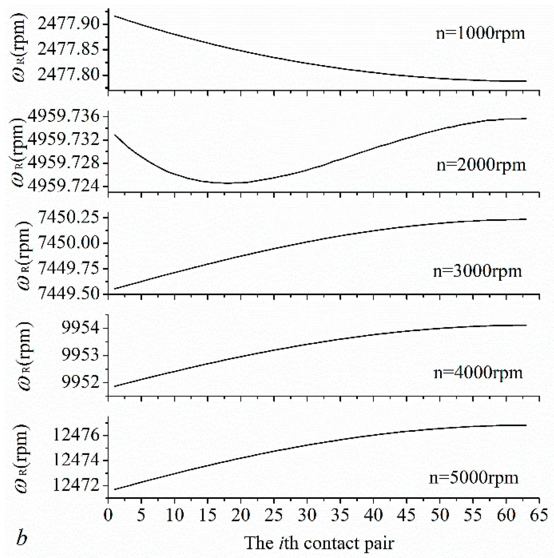
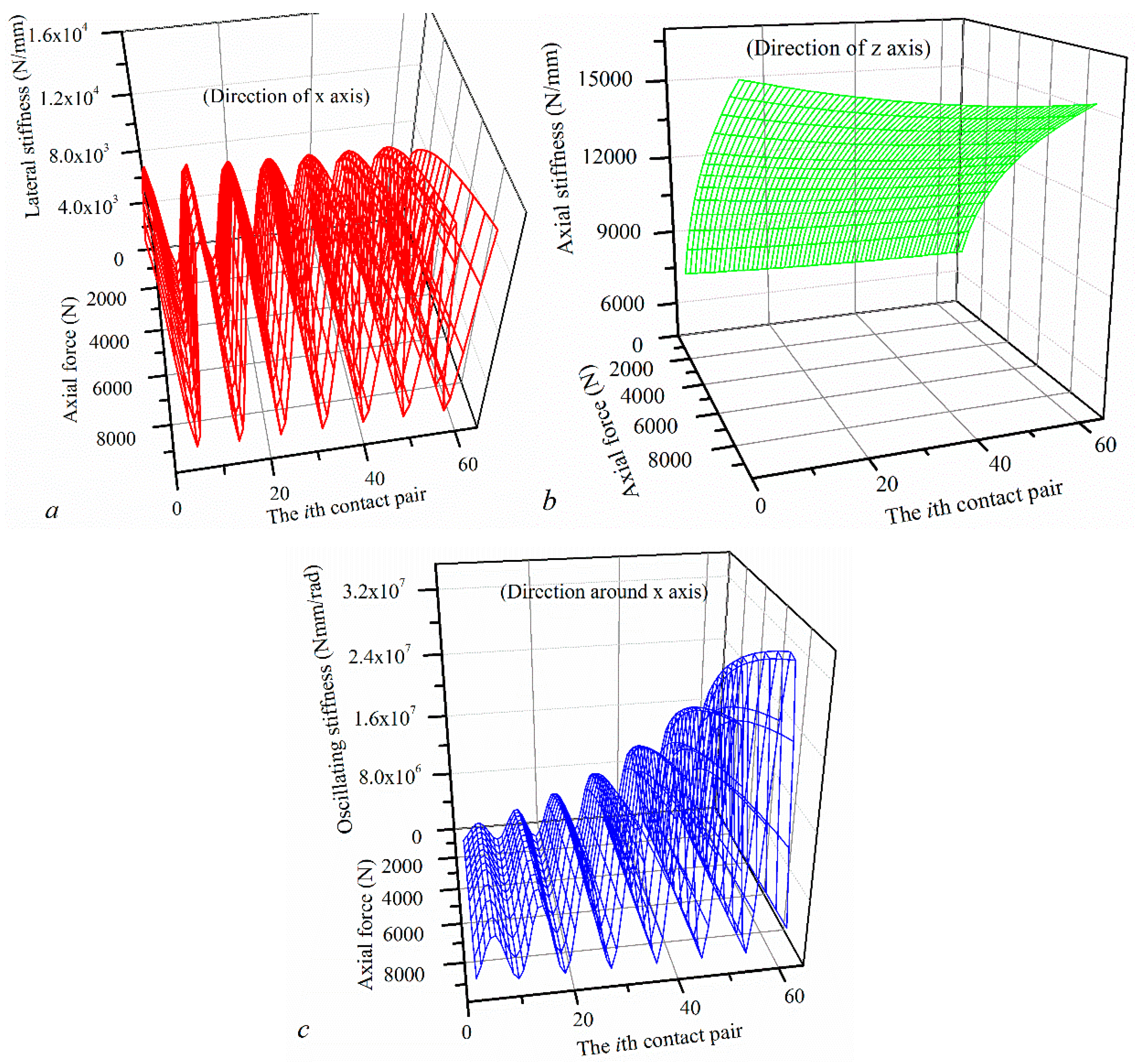
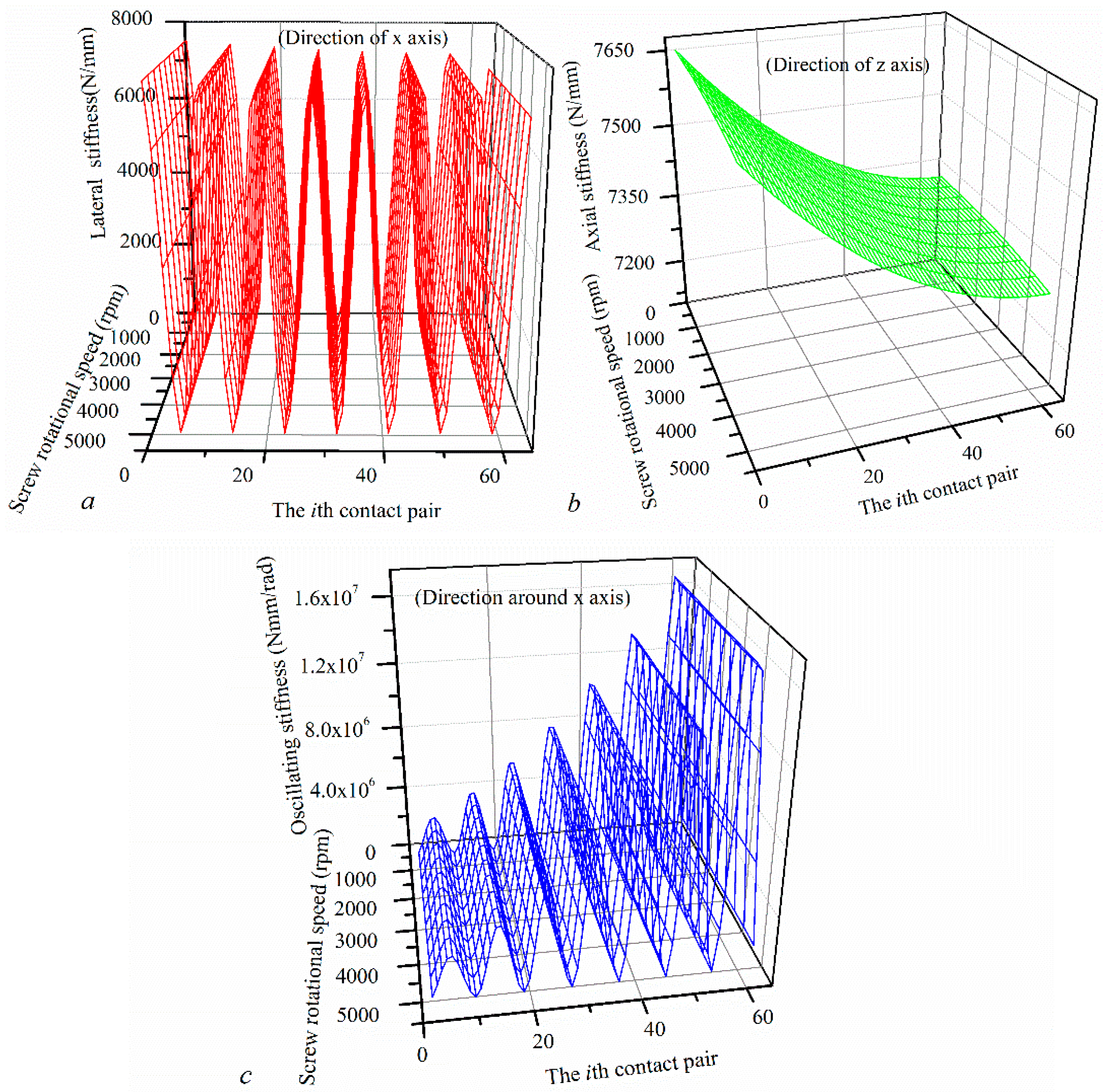
3.2. Variation of Dynamic Contact Normal Force

When the screw speed is 0, friction is not considered, $Q_{Si}=Q_{Ni}=Q_i$. In a previous study, it was shown that the normal forces decrease with the contact pair departing from the load end of the SNBSP. The normal forces of the ball increase simultaneously with axial force increase [12].

However, in the dynamic state, $Q_{Si}\ne Q_{Ni}$. Figure 10 shows the variation of the dynamic contact force with the contact pair position and the screw speed when the axial force is 1000 N. Firstly, it is obvious from Figure 10 that the normal contact force of the nut is greater than that of the screw in the same position, and the higher the screw speed is, the greater the difference is. In different contact position, the contact force difference between the nut and screw is not the same; when the screw speed is below 1500 rpm, with the contact position moving backwards, the contact force difference between the nut and screw gradually decreases. When the screw speed is below 500 rpm, though still conforming to this rule, the relative deviation is less than 0.05%, therefore, it is considered that the screw and nut contact force are approximately the same at the speed below that speed. However, when the screw speed of the screw is higher than 1500 rpm, the contact force difference between the nut and the screw increases gradually as the contact position moves behind. The higher the screw speed, the more obvious this phenomenon.

Secondly, it is consistent with the uneven distribution static contact force that the dynamic contact force decreases from the first contact pair to the last one. When screw speed increases, the level of uneven load distribution of screw increases slightly but that of the nut decreases. When the axial force is 1000 N, the screw speed is 500 rpm, the first and the last contact force ratio of the screw is 1.1422, and that of the nut is 1.1427. When the screw speed reaches 5000 rpm, the ratio of the screw is 1.1427, and that of the nut reduces to 1.1387.

Figure 11a,b exhibit variation of contact normal force with the contact position and the axial force when the screw speed is 2000 rpm. It is clear that, when the axial force increases, the uneven load distribution of both screw and nut are gradually increased.

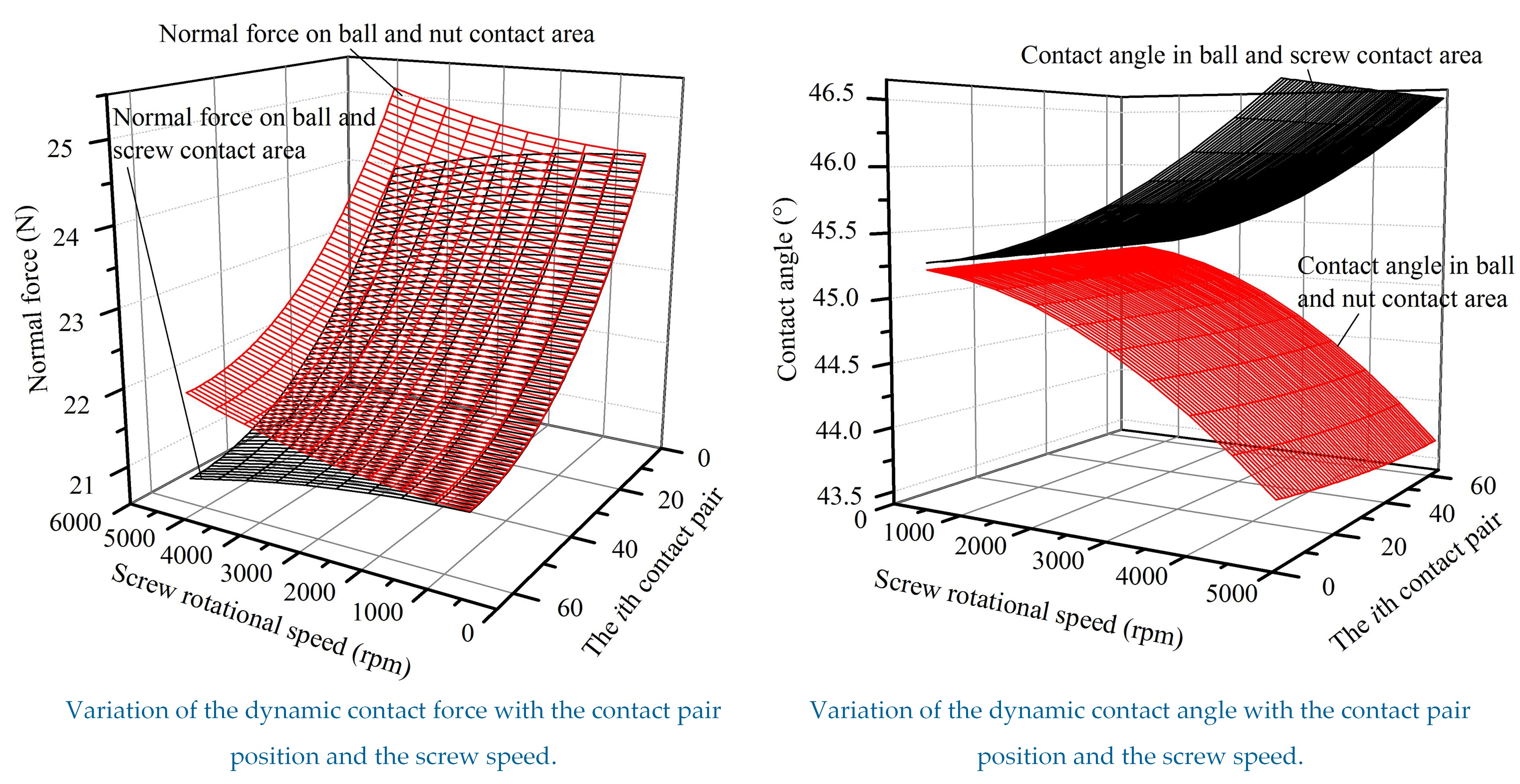
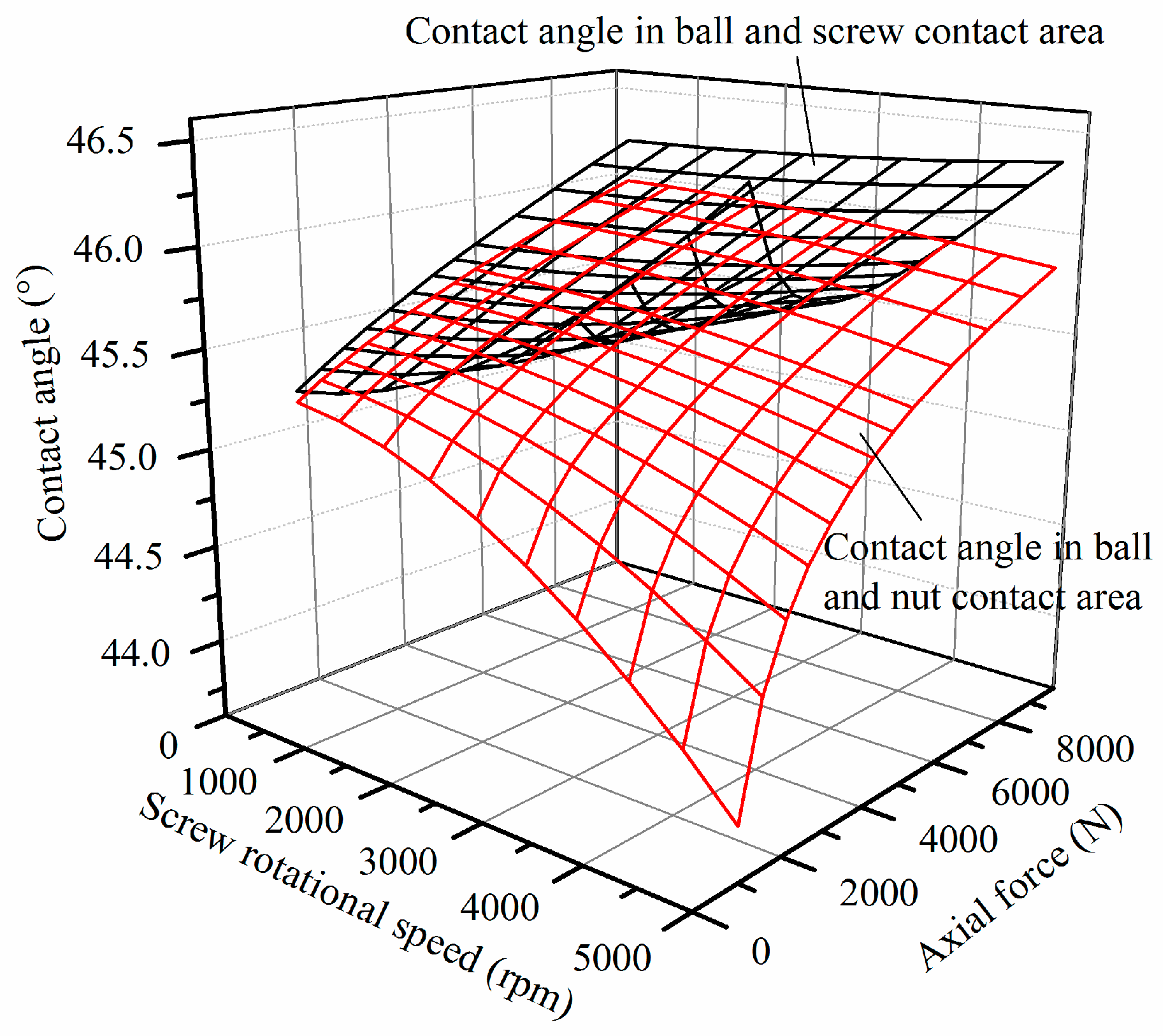
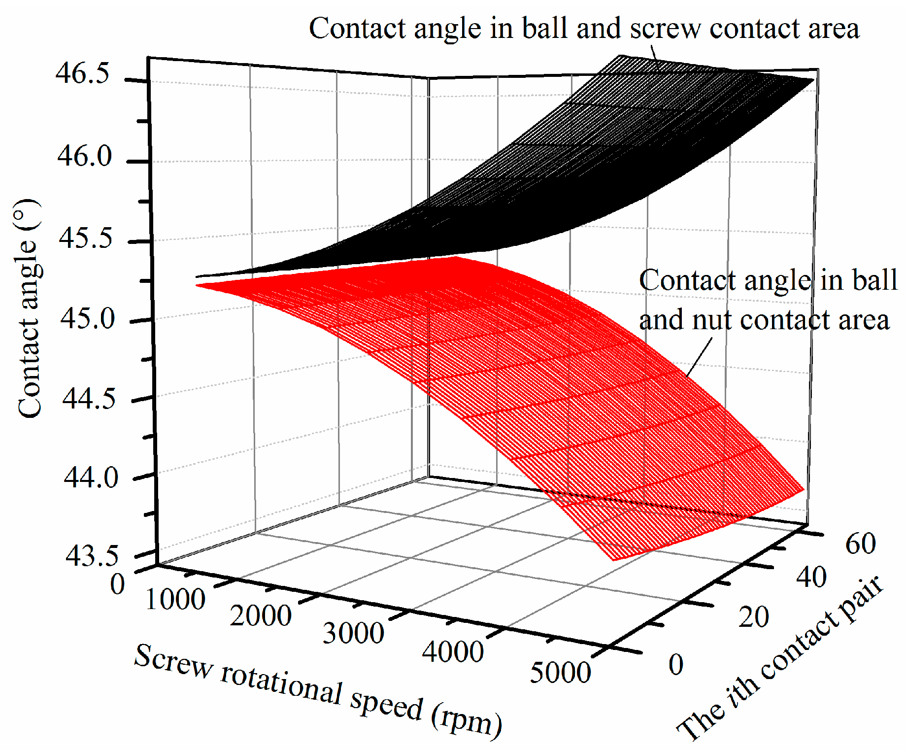
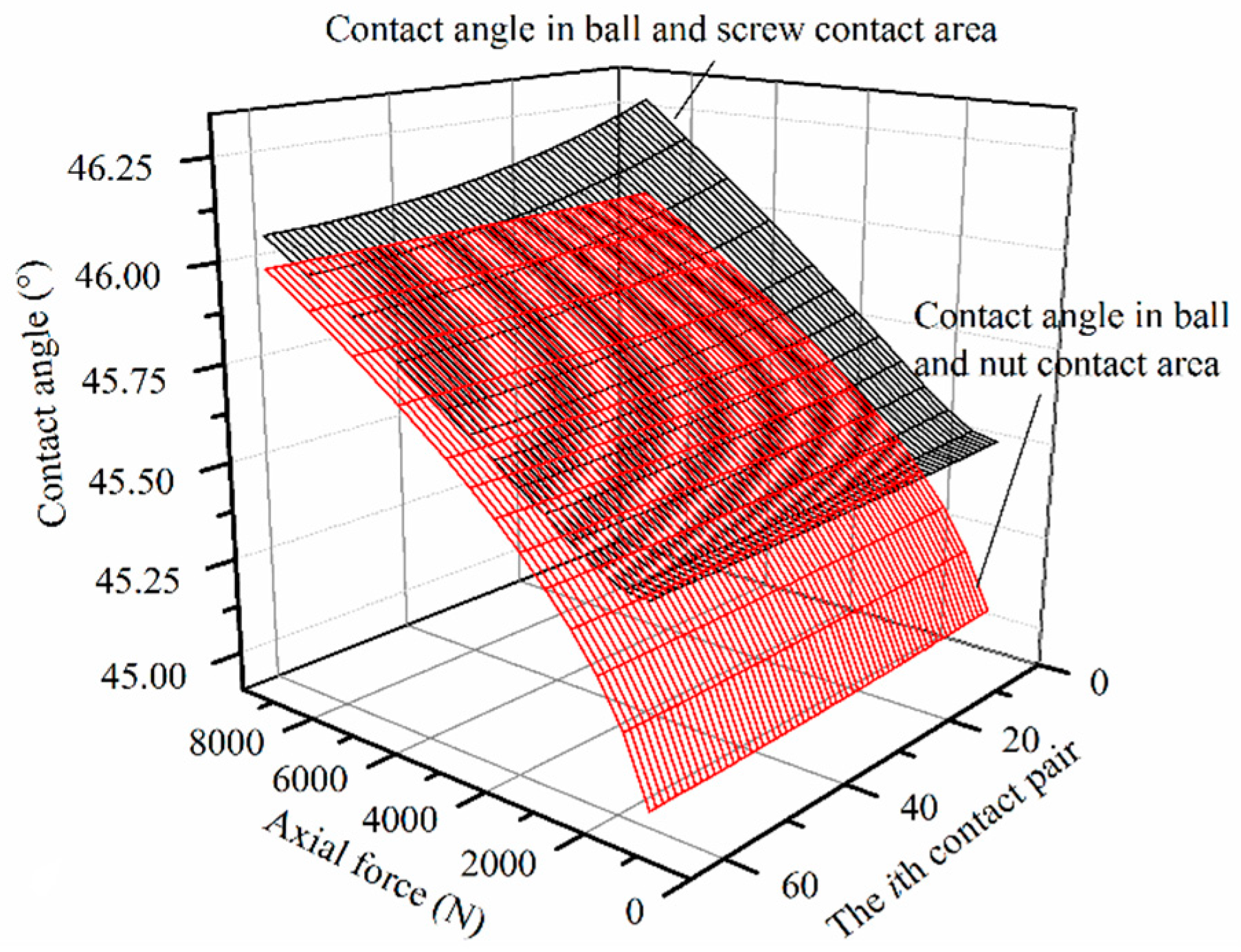
3.3. Variation of Dynamic Contact Angle

Figure 12 illustrates the variation of the dynamic contact angle of the first contact pair with axial force and screw speed.

It is clear that under the same axial force, the screw dynamic contact angle increases with the screw speed increase. However, the variation of dynamic contact angle of the nut is just the opposite. The contact angle of the nut increases with the axial force increase. When the screw speed is lower than 2000 rpm, the contact angle of the screw increases with the increase in axial force. But when the speed of the screw is higher than 2500 rpm, it decreases first and then increases with the increase in axial force. This is because the factor of screw speed has a coupling effect on the dynamic contact angle. At the same time, it can be seen that the higher the screw speed is, and the smaller the axial force is, the greater the difference in the contact angle between the screw and the nut. However, the lower the screw speed is, and the smaller the axial force is, the closer the two dynamic contact angles.

Figure 13 shows the variation of dynamic contact angle with the contact position and the screw speed when the axial force is 1000 N. At the same speed of screw, the dynamic contact angles of screw and nut both decrease from the first contact pair to the last one. However, the characteristics of the two are not the same. The uneven distribution of the dynamic contact angle of the screw is not obvious with the increase in the screw speed, while that of the nut is opposite.

The reason is that the ball’s spinning angle velocity (${\omega }_R$) and revolutional angle velocity (${\omega }_m$) are the two important factors which affect the dynamic contact angle. The bigger the two velocities are, the greater the screw contact angle is and the smaller the nut contact angle is. Figure 14a illustrates the variations of ${\omega }_R$ and ${\omega }_m$ with screw speed under different axial force. It is obvious that both two angle velocities are almost linear with screw speed. The axial force has little effect on the two angular velocities. Figure 14b shows variations of ${\omega }_R$ with the contact position. It is clear that when the screw speed is higher than 2000 rpm, ${\omega }_R$ increases from the first contact pair to the last one. When the screw speed is higher than 4000 rpm, ${\omega }_m$ increases from the first contact pair to the last one. Normal contact force decreases with variation of the contact position, which is also the positive factor that makes the contact angle change with the screw speed. All of these factors make the distribution of the dynamic contact angle of the screw less obvious but that of the nut more obvious.

Figure 15 demonstrates the dynamic contact angle variation of the screw and nut with the contact position and axial force when the screw speed is 2000 rpm, respectively.

For the contact pairs in the same position, both the screw and nut dynamic contact angles increase with the axial force increase. For contact pairs in different position, dynamic contact angle decreases with the contact pair position changing, which presents the phenomenon of uneven distribution. Under the same axial force, the uneven distribution of the screw dynamic contact angle is more significant. However, as the axial force increases, the uneven distribution of the dynamic contact angles of the lead screw will be more and more significant, while that of the nut is contrary.

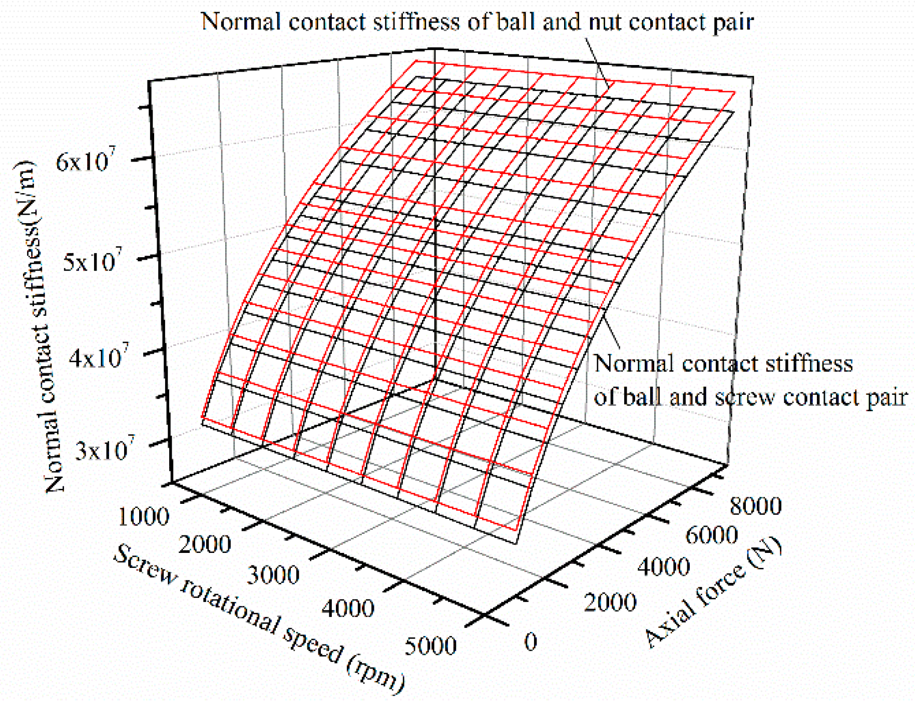
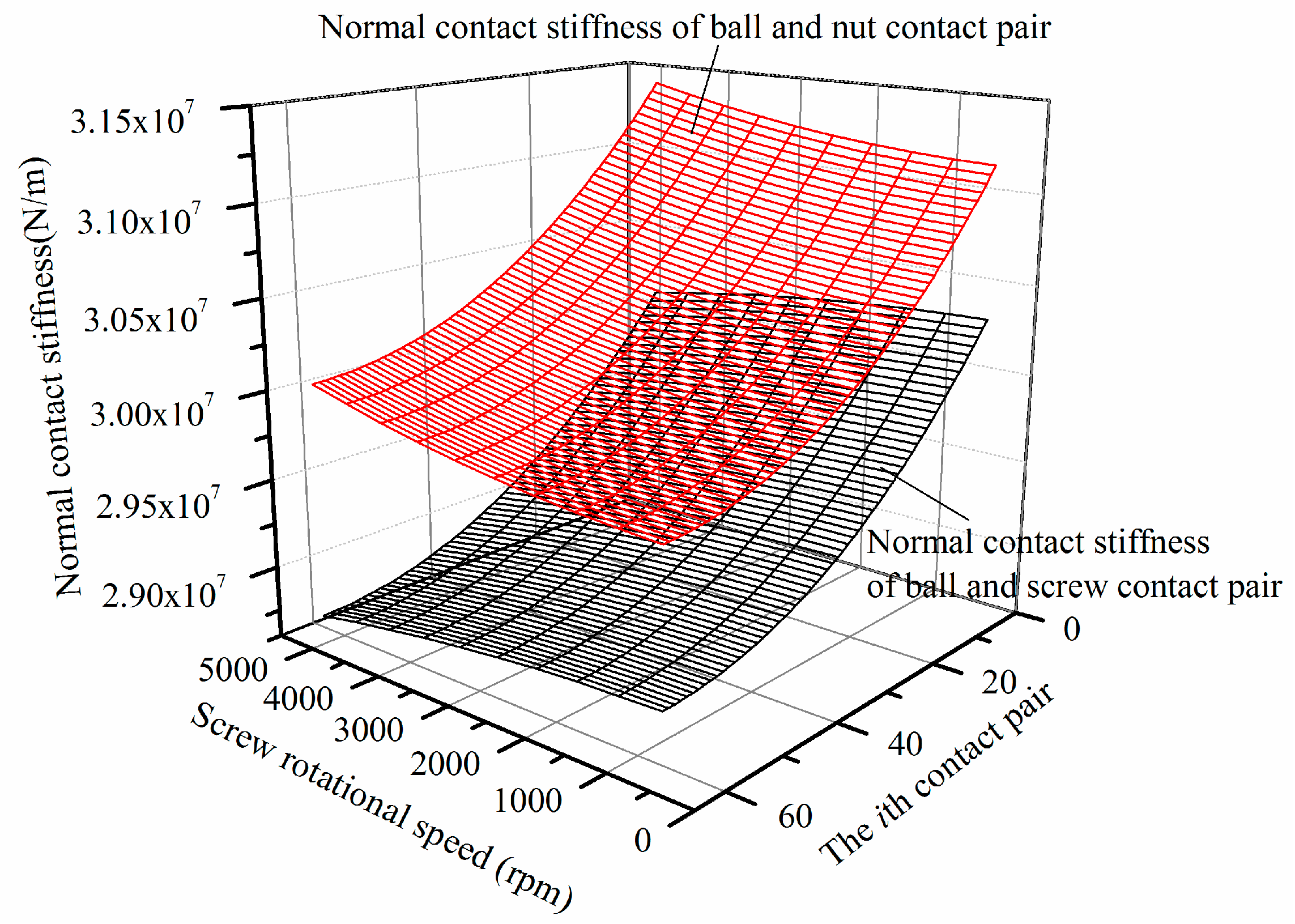
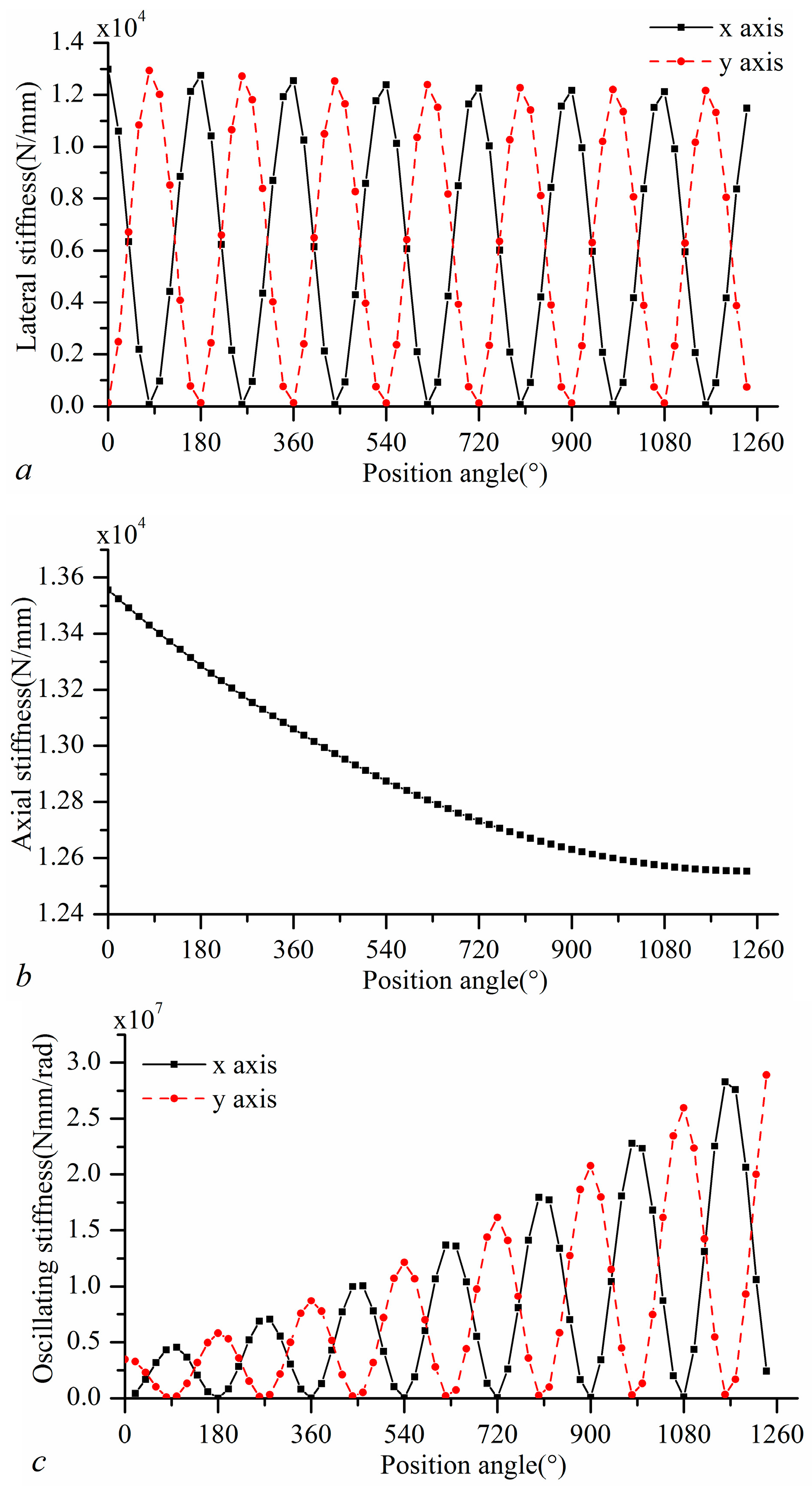
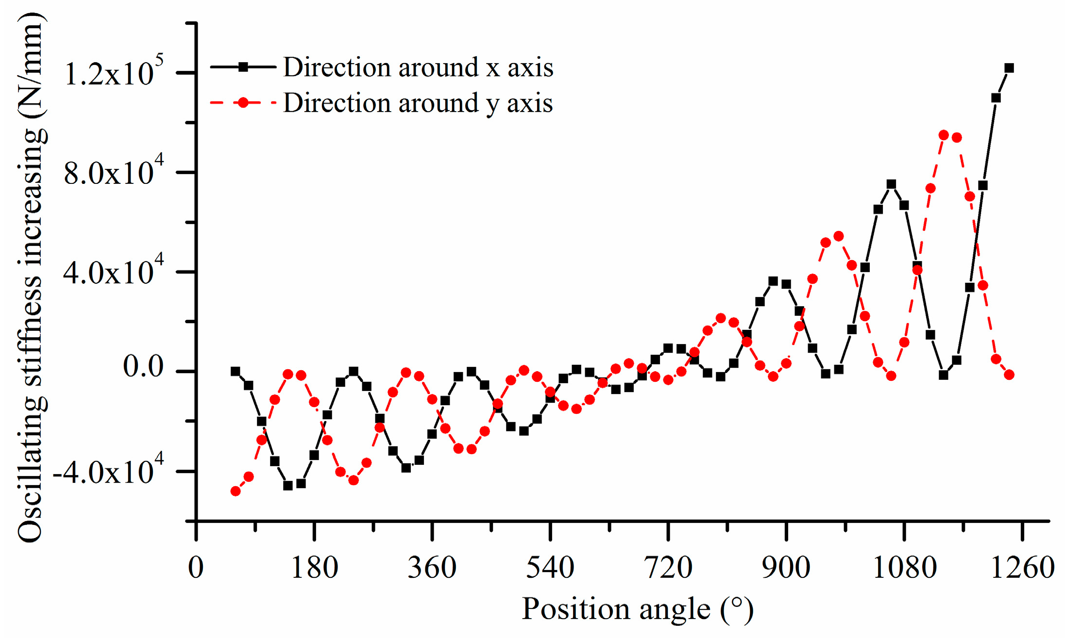
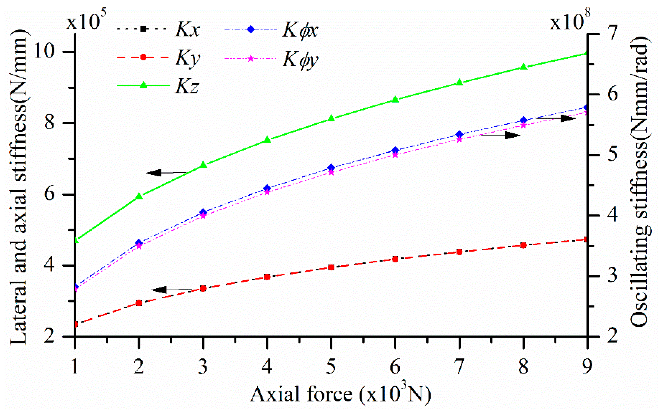
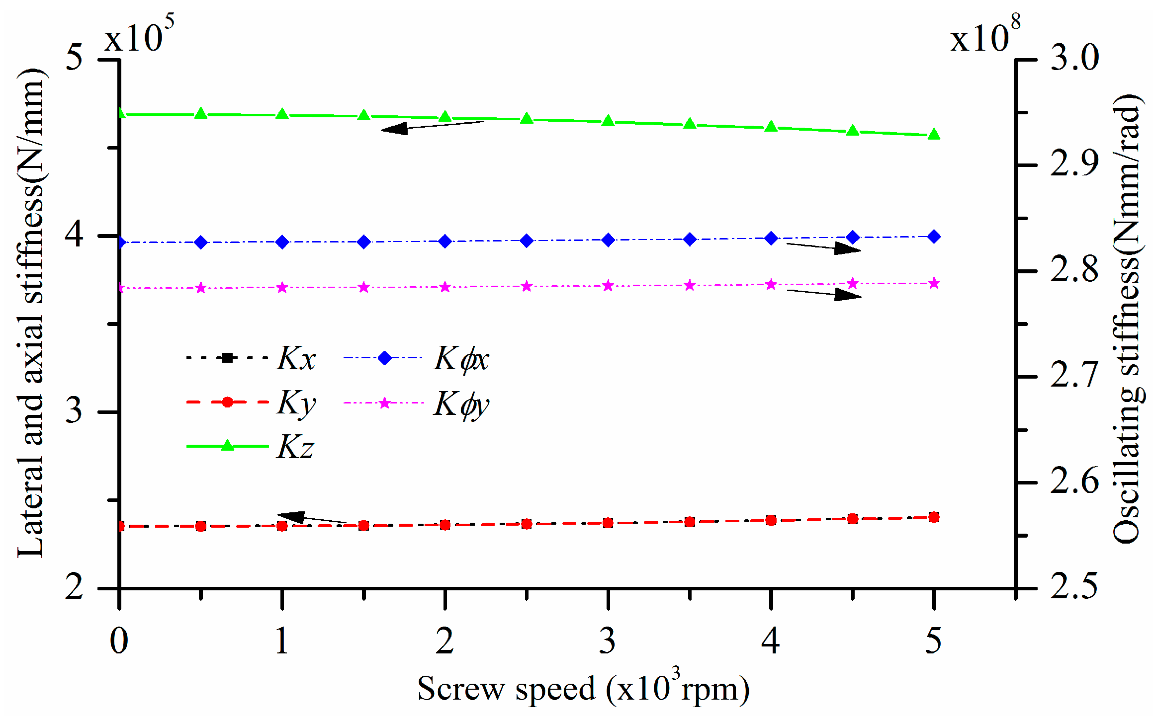
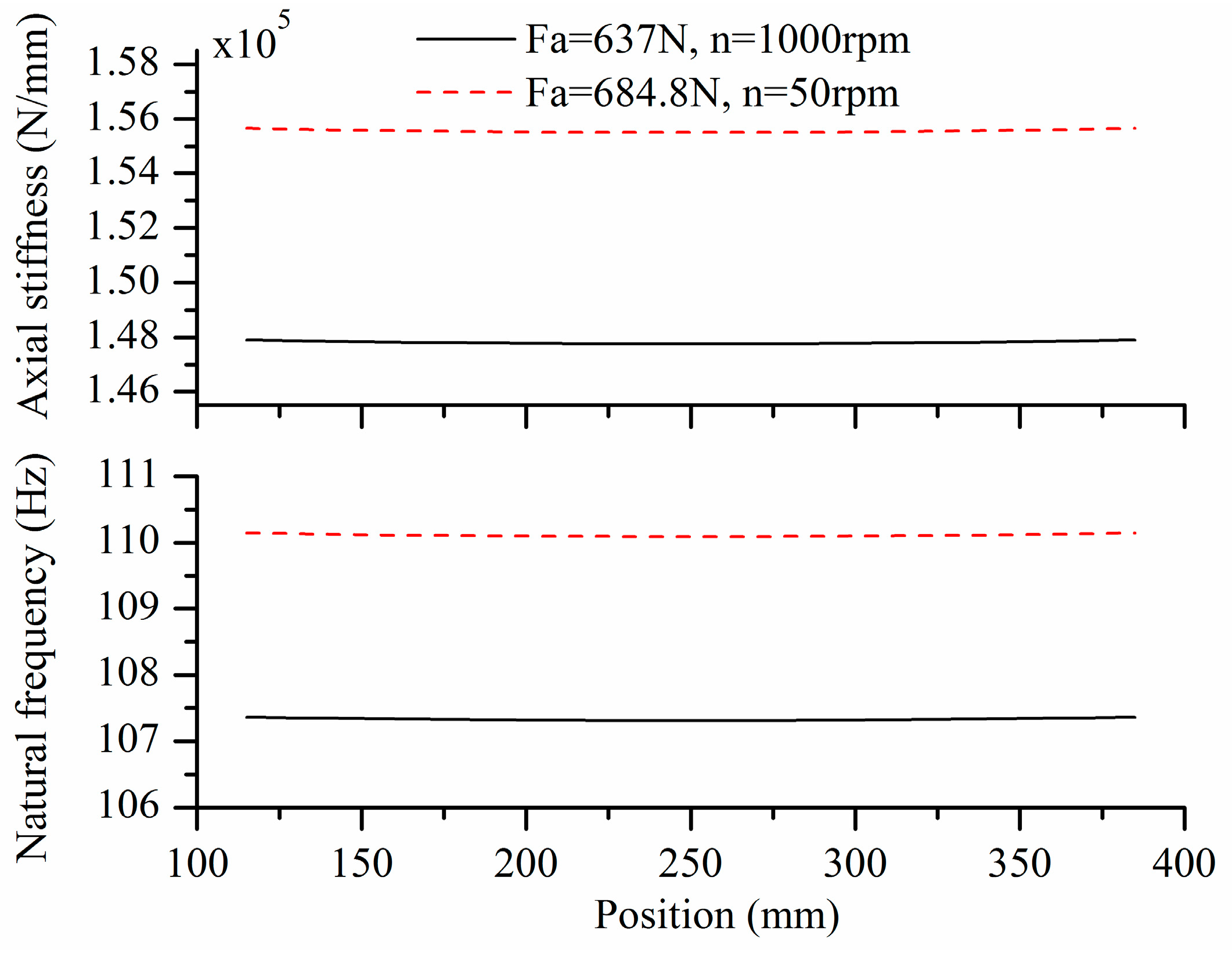
3.4. Variation of Dynamic Contact Stiffness

Substituting $Q_{\varsigma i}^{}$ into Equation (41), normal stiffness $k_{\varsigma i}$ will be calculated. Figure 16 reveals the variation of the normal stiffness of the first contact pair with the axial force and the screw speed, respectively. It can be seen from the figure that the general variation rules of the screw and nut’s normal contact stiffness are consistent. The normal contact stiffness increases as the axial force increases. The normal contact stiffness of the screw is less than that of the nut. With the screw speed increase, the normal contact stiffness decreases gradually, but the influence of the screw speed on the contact stiffness is less than that of the axial force.

Figure 17 exhibits variation of the normal contact stiffness with the screw speed and the contact position when the axial force is 1000 N. It is obvious that as the contact position is moving backward, the normal contact stiffness of both the screw and nut decreases gradually. In the same position, the normal contact stiffness is gradually reduced with the screw speed increase. The nut normal contact stiffness is always greater than screw.

In the static state, the ball screw local contact stiffness in five directions can be calculated through Equations (42), (43) and (45). Figure 18 exhibits the variation of the local stiffness with contact position; the local lateral stiffness and oscillating stiffness fluctuate with the period of π and the phase difference of π/2. The amplitudes of lateral stiffness decrease slightly with the contact pair position far away from the SNBSP load side, but that of oscillating stiffness increases, as illustrated in Figure 18a,c. The load axial stiffness decreases with the contact pair position far away from the SNBSP load side, as shown in Figure 18b.

Figure 19 demonstrates the variation of ball screw dynamic local contact stiffness with contact position and axial force when the speed of the screw rotational is 2000 rpm. The variation of dynamic contact stiffness with the contact position in all directions are consistent with them in A static state. It can be noted that single ball local stiffness depends upon the normal force, hence all of the local stiffness increases with the increase in the axial force.

Figure 20 exhibits the variation of the local contact stiffness with the contact position and the screw speed when the axial force is 1000 N. From Figure 20a, it can be seen that the lateral stiffness increases gradually with the increase in the screw speed. The main reason for this phenomenon is that with the increase in screw rotational speed, the spinning and revolution angular velocities of the ball increase, and the ball moves to the outside gradually, which means that the nut contact angle decreases and the screw contact angle increases slightly. A closer contact state between the ball and the screw and nut raceway is generated, which leads to stronger support ability in the lateral direction. Therefore, lateral stiffness becomes bigger.

Figure 20b illustrates the variation of the local axial stiffness with the screw speed and the contact position. As the contact position moves backwards, the local axial stiffness decreases gradually. However, as the screw speed increases, the axial local stiffness gradually decreases. The reason for this is mainly that the screw and nut’s normal contact stiffness decreases with the screw speed’ increase. On the other hand, because the ball and raceway form a more close contact state which is caused by the changing of the contact angle, it leads to a stronger supporting ability along the lateral direction, and the axial support ability will decrease.

Figure 20c exhibits the variation of the local oscillating stiffness with the screw speed and the position of the contact pair. It is different from lateral and axial stiffness that when the screw speed increases, the oscillating stiffness of the first three turns decreases, but the amplitude of the decrease gradually decreases with the phase fluctuation. The fourth half turn is a transition stage. From the fifth half turn, the contact pair oscillating stiffness increases gradually, and the amplitude of the increase gradually increases with the phase fluctuation. Figure 21 shows the difference value between the local oscillating stiffness of each contact pair at screw speeds of 5000 and 500 rpm when the axial force is 1000 N.

Substituting local stiffness into Equation (46), and the screw-nut pair global stiffness will be calculated. As shown in Figure 22, the global contact stiffness in all directions increased with the increase in the axial force. Compared with the lateral stiffness $K_x$ and $K_y$, the axial stiffness $K_z$ and the oscillating stiffness $K_{\varphi x}$, $K_{\varphi y}$ increase more significantly, which indicates that the effect of the axial force on the latter two is more significant.

Figure 23 exhibits the global stiffness varying with screw speed when the axial force is 1000 N. It is clear that with the rotating speed of the screw increase, the lateral stiffness $K_x$ and $K_y$ increase monotonically, while the axial stiffness $K_z$ decreases monotonically, which is in accordance with variation rule of the local contact stiffness. The oscillating stiffness $K_{\varphi x}$ and $K_{\varphi y}$ increase with screw speed increasing. Although the local oscillating stiffness of the first 1.5 turns decreases with screw speed increasing, it increases with the screw speed, increasing two cycles, and the increment is significant. So the total value of the oscillating stiffness increases monotonically, but it is clear that the amplitude of its increase is not very obvious.

4. Sensorless Stiffness Estimating Method Based on Contact Stiffness Model and Experimental Verification

4.1. Sensorless Stiffness Estimating Method Based on Contact Stiffness Model

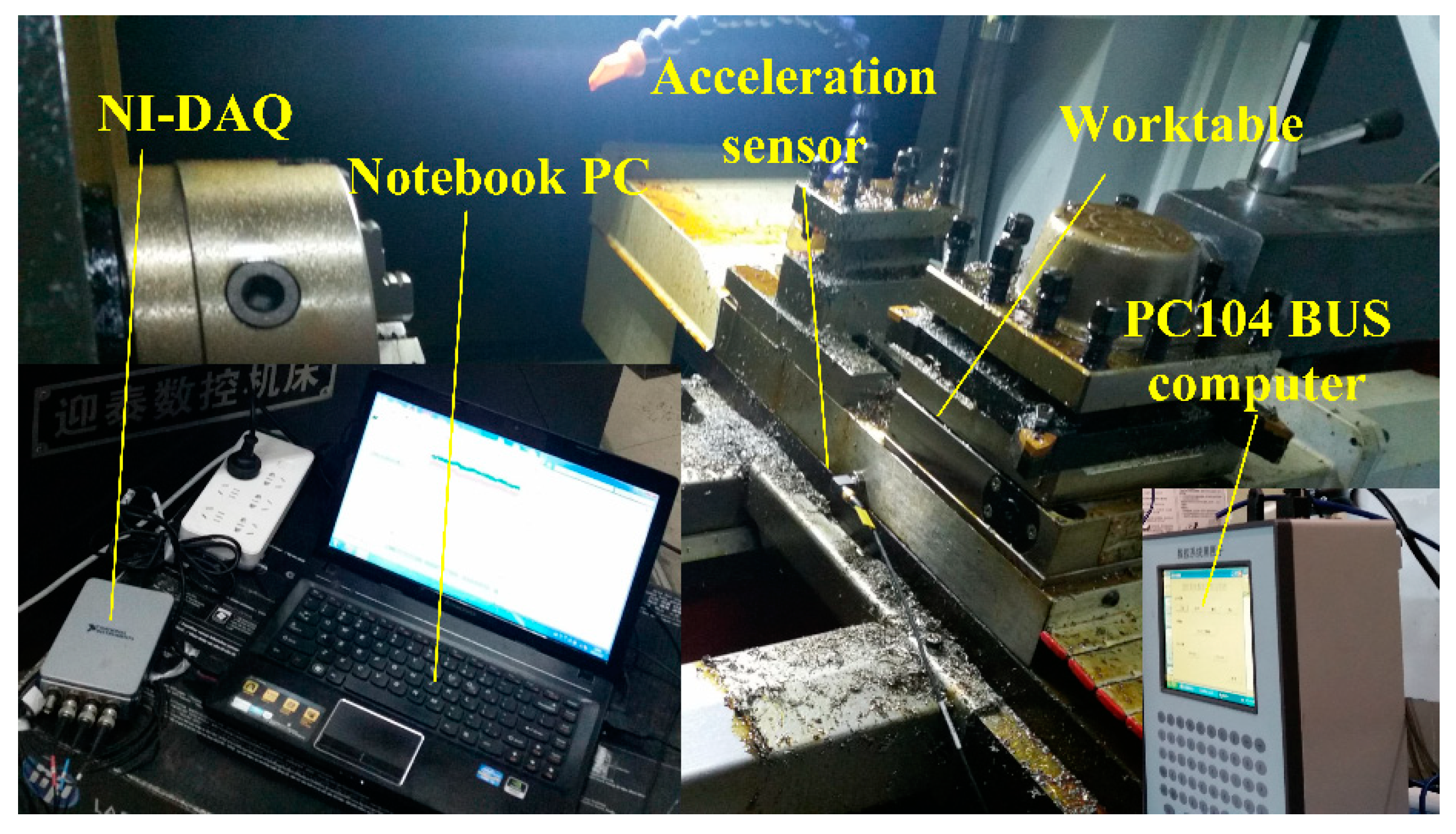
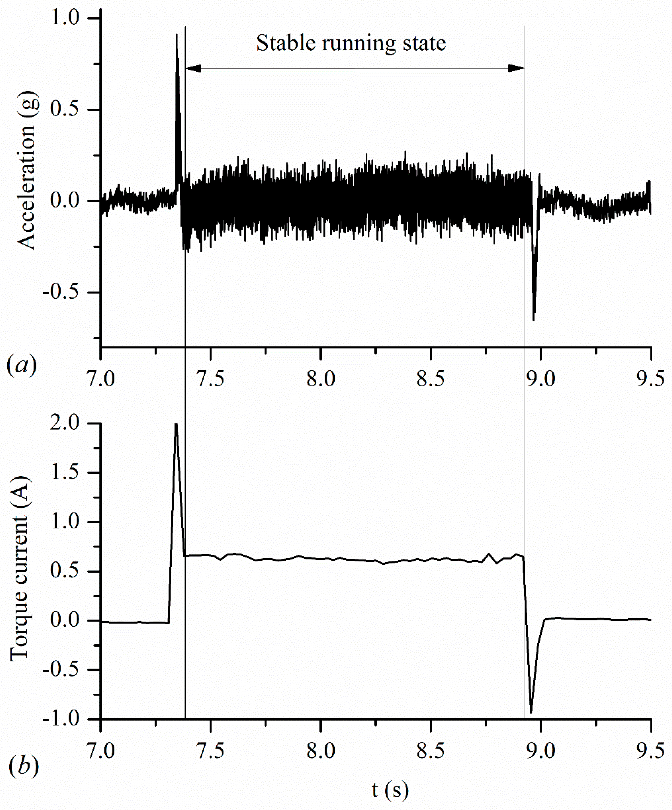
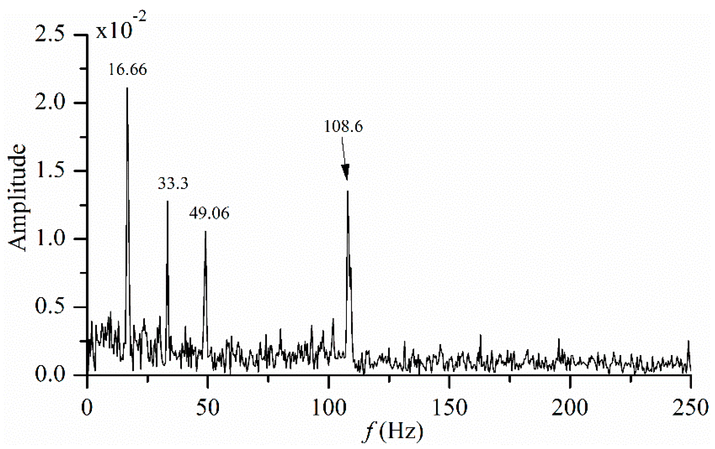
Through the numerical analysis of the dynamic contact model, it is clear that the axial force and the speed of the screw have major influence on the dynamic contact stiffness of the SNBSP. At the same time, they are also important parameters to solve the model. If the values of them can be obtained when the machine tool is running, we can solve the dynamic contact stiffness of SNBSP according to the dynamic model proposed in this paper. It is significant to evaluate the dynamic characteristics of mass production CNC machine tools. The value of screw speed can be obtained through the CNC program. But the capture of axial force needs the help of an external sensor generally. That is why the stiffness analysis can only be carried out on components or a special test bench in references.

The relationship between the axial force of the SNBSP and the screw torque is as follows [21,22]

$$F_a=\frac{2\mathsf{\pi }\eta T_{\mathrm{d}}}{L_p}$$

(47)

where F_a denotes the axial force. $T_{\mathrm{d}}$ is the driving torque. L_p is the lead of the screw. $\eta$ is the transmission efficient of SNBSP. The specific solution process can be seen in the Appendix A.

The relationship between the torque T_d and torque current of servo motor (TCSM) is as follows

$$T_{\mathrm{d}}=k_{\mathrm{e}}\cdot i$$

(48)

where $k_{\mathrm{e}}$ is the servo motor torque constant; i is the TCSM.

In this way, the problem of capturing the axial force is transformed into the problem of capturing the TCSM.

In a previous study, we developed a collection program by using VC + +. The working data of CNC system can be collected in real time through FOCAS1 database [23]. If the same type of data is collected, the sampling frequency can reach 28 Hz. For a more detailed processing, refer to reference [23]. In this way, an Ethernet cable is used to connect the CNC system with the PC, and then the TCSM signals at any time can be captured without the help of any external sensor. (Notes: A notebook PC was used in the earlier stage of study. However, it was replaced by a PC104 BUS computer for other functions.).

The process of estimating the dynamic contact stiffness of ball screw without a sensor can be seen in Figure 24.

4.2. Experiment

In order to verify the numeric results of the dynamic contact model and sensorless stiffness estimating method, an experiment is conducted to measure the axial stiffness of a SNBSP in the Z-axis feed system of a CNC lathe (Shenyang Machine Tool Group, Shenyang, China) with Fanuc Series (Figure 25). The experimental lathe parameters are exhibited in

Table 2. Specific parameters of experimental CNC lathe.

Parameters	Value	Unit
I. Geometric parameters of feed system
orktable mass mt	325	Kg
Axial stiffness of fixed end bearing $K_b$	2 × 108	N/m
The length of the screw	500	mm
The travel of the feed system	300	mm
Motor torque coefficient	1.85	Nm/A
Elastic modulus of screw shaft Es	210	GPa
II. Operating conditions
Feed speed	10,000	mm/min
	500	mm/min
Two end point coordinates
Z0	15	mm
Z1	285	mm

. The parameters of SNBSP(Best Precision, Jining, China) are exhibited in Table 1.

In order to verify this, an external sensor is needed to measure the response signals during the operation of the machine tool. Fast Fourier transform (FFT) is used to process the signals, and the frequency components obtained are compared with the theoretical values to verification.

Hence an acceleration sensor, B&K4520-004 (Brüel & Kjær, Nærum, Denmark), of which the maximum of sampling frequency is 25.6 kHz, was mounted on the worktable and moves together with it. The acceleration sensor was connected to NI-DAQ (National Instruments, Austin, TX, USA) which was connected to Notebook PC. The max travel of the worktable is 300 mm. However, considering the safety of high-speed operation, the travel was set to 270 mm with two end point coordinates 15 mm (denoted by Z0) and 285 mm (denoted by Z1), respectively.

The experimental process is as follows.

• Step 1: Locate the worktable at the given position Z1 by using a NC program.
• Step 2: Run acceleration sensor data acquisition program. Run servo axis data acquisition program to capture the TCSM.
• Step 3: Run the NC program. The worktable moves from Z1 to Z0 at the specified speed.
• Step 4: All the application programs are stopped and the data are saved.

Because the maximum feed speed of the Z feed shaft of the NC lathe is locked to 10,000 mm/min, and the lead of the Z axis screw shaft is 10 mm, that means that the screw speed is 1000 rpm. Hence, the high speed of the screw is selected as 1000 rpm, and 50 rpm is selected as the low speed. Under each rotating speed, the worktable is run three times according to the above test steps, in the forward (Z1–Z0) and reverse (Z0–Z1) direction. Then, the acceleration and TCSM signals are obtained. Figure 26 shows the acceleration and TCSM signals of the first positive feed at the screw speed 1000 rpm. It can be seen from Figure 26a that there are three states in the process: a state of acceleration, stable running and deceleration. The acceleration signals in the stability state can be used for FFT analysis.

It can be seen from Figure 26b that there are also three operation states in TCSM signals. Calculate the average value of the TCSM in the stability state. By substituting the average value of the current into Equations (47) and (48), the axial force of the Z axis screw of the feed system can be obtained as 637 N under the screw speed of 1000 rpm. According to the model presented in this paper, the dynamic axial contact stiffness of the SNBSP can be calculated. When the screw speed is 50 rpm, the axial force is about 684.8 N. Because the speed is very low, the axial stiffness of the SNBSP can be solved by static model, and the result is 3.89 × 10⁵ N/mm.

Figure 27 shows the configuration of the z-axis feed system and the dynamic model. The mounting method of ball screw is fixed-fixed, as shown in Figure 27a. The stiffness values of the frame and worktable of the experimental machine tool are all large. Compared with the worktable mass, the mass of the screw can be neglected. Especially, low screw lead reduces the influence of the torsional stiffness and moments of inertia of the screw and other rotating parts. Therefore, the dynamic model of the worktable is simplified as in Figure 27b.

The stiffness of the system is expressed as follows:

$$\frac{1}{K_f}=\frac{1}{\frac{1}{\frac{1}{K_b}+\frac{1}{K_{s0}}}+\frac{1}{\frac{1}{K_b}+\frac{1}{K_{s1}}}}+\frac{1}{K_p}$$

(49)

where $K_b$ denotes the axial stiffness of fixed end bearing. $K_p$ denotes the axial stiffness of the screw–nut pair, which means that $K_p=K_z$. $K_{s0}$ and $K_{s1}$ denote the axial stiffness of the screw shaft on both sides of the nut, with

$$K_{s\chi }\doteq \frac{\pi {\left(d_m-d_B\right)}^2{E}_s}{L_{\chi }}$$

(50)

where $L_{\chi }$ denotes the distance between the nut and the two fixed ends, $\chi =$0 or 1.

Then the feed system natural frequency is expressed as [24]:

$$f_{\mathrm{n}}=\frac{1}{2\pi }\sqrt{\frac{K_f}{m_t}}$$

(51)

The axial stiffness of the feed system can be determined by numeric iteration of Equations (49) and (50).

It is clear from Equation (50) that the screw shaft axial stiffness varies with the position of the worktable, so the axial stiffness and natural frequency of the feed system are also time-varying. The theoretical value of the axial stiffness and natural frequency of the feed system variation with the position of the worktable under the experimental conditions are shown in Figure 28. It can be seen that although the axial stiffness and natural frequency vary with the position of the worktable, the variation is not obvious. For example, when the screw speed is 1000 rpm, the axial stiffness variation ratio is 0.087%, while the natural frequency variation ratio is only 0.046%. Therefore, the axial stiffness and natural frequency of the Z axis of the feed system can be considered to be approximately the same in different positions.

The feed system natural frequency will be calculated by Equation (51). Herein, the contact stiffness and the natural frequency determined above are considered to be theoretical values of them, respectively.

On the other hand, the FFT algorithm is carried out to investigate the spectrum characteristics of the worktable acceleration. In Figure 29, the FFT results of the worktable acceleration are represented in the stable running state in Figure 26a. It is obvious that the 16.66 Hz and its two and three times harmonic frequency components are the frequency components corresponding to the screw speed of 1000 rpm, and there are several frequency components at the low frequency section. In fact, the feed system has shapes of many modes [10], and so the FFT results of its vibration contain multiple frequencies. However, the first mode of the feed system is generally axial [25]. Herein, the frequency in Figure 29, 108.6 Hz, should be the natural frequency, whose corresponding mode should be the axial vibration of the worktable. Therefore, 108.6 Hz corresponds to the natural frequency $f_{\mathrm{n}}$ in Equation (51).

The theoretical and experiment values of the feed system dynamic parameters under the two screw speeds in Section 4.1 are exhibited in

Table 3. Theoretical and test values of feed system dynamic parameters.

Screw Speed (rpm)	Direction	Theoretical Value				Measured Value
		${\mathit{F}}_{\mathit{a}}\left(\mathbf{N}\right)$	${\mathit{K}}_{\mathit{p}}(\mathbf{N}/\mathbf{m})$	${\mathit{K}}_{\mathit{f}}(\mathbf{N}/\mathbf{m})$	${\mathit{f}}_{\mathbf{n}}\left(\mathbf{Hz}\right)$	$\mathit{f}\left(\mathbf{Hz}\right)$
1000	Z1—Z0	636.8	3.439 × 108	(1.4790~1.4776) × 108	107.31~107.36	108.3
		635.6	3.439 × 108	(1.4790~1.4776) × 108	107.31~107.36	108.6
		637	3.439 × 108	(1.4790~1.4776) × 108	107.31~107.36	108.5
	Z0—Z1	637	3.439 × 108	(1.4790~1.4776) × 108	107.31~107.36	108.4
		635.6	3.439 × 108	(1.4790~1.4776) × 108	107.31~107.36	108.6
		637.5	3.439 × 108	(1.4790~1.4776) × 108	107.31~107.36	108.5
50	Z1—Z0	684.8	3.89 × 108	(1.5551~1.5566) × 108	110.09~110.15	112.1
		683.6	3.89 × 108	(1.5551~1.5566) × 108	110.09~110.15	111.8
		684.8	3.89 × 108	(1.5551~1.5566) × 108	110.09~110.15	112.1
	Z0—Z1	684.8	3.89 × 108	(1.5551~1.5566) × 108	110.09~110.15	112.1
		684.8	3.89 × 108	(1.5551~1.5566) × 108	110.09~110.15	112.2
		685.6	3.89 × 108	(1.5551~1.5566) × 108	110.09~110.15	112.2

. The results show that the theoretical values of natural frequency are consistent with the measured values. This fact verifies the effectiveness of the whole rolling elements dynamic contact model and sensorless stiffness estimating method proposed in this paper. This estimating method can be widely used in the mass production CNC machine tools.

5. Conclusions

In this paper, the dynamic contact mechanics model and dynamic contact stiffness model of all balls of screw–nut pairs are established. Based on this, a sensorless stiffness estimating method is proposed. The following conclusions are obtained:

(1) In the dynamic state, $Q_{Si}\ne Q_{Ni}$. In the same position, the normal contact force of the nut is greater than that of the screw. The higher the speed of the screw, and the larger the axial force, the greater the difference between the two normal forces. When the screw speed is below 500 rpm, it is considered that the contact normal force of the screw and nut are approximately the same. Screw speed has different effects on the uneven distribution of the load of the screw and nut.

(2) In the dynamic state,${\alpha }_{\mathrm{s}i}\ne {\alpha }_{\mathrm{n}i}$. In the same position, the contact angle of the screw is greater than that of the nut. The higher the speed of the screw, and the smaller the axial force, the greater the difference between the two contact angles. Because the spinning and revolutional angle velocities of the ball are different at different contact positions, the coupling influence of the axial force and screw speed have different effects on the uneven distribution of the dynamic contact angle of the screw and nut.

(3) The effect of the screw speed on the lateral stiffness and axial stiffness is more significant, but the influence on the oscillating stiffness is little. However, the influence of the axial force on all the stiffnesses is significant.

(4) A stiffness sensorless estimating method of SNBSP was proposed. The axial force of SNBSP in feed system can be captured without a sensor when the machine tool is running. Then, the stiffness of SNBSP can be obtained. This method is verified by an experiment. Hence it is an effective method which can be used in mass production CNC machine tools.

References

1. Frey, S.; Walther, M.; Verl, A. Periodic variation of preloading in ball screws. Prod. Eng. Res. Devel. 2010, 4, 261–267. [Google Scholar] [CrossRef]
2. Shimoda, H.; Ando, Y.; Izawa, M. Study on the Load Distribution in the Ball Screw (1st Report). Manu. Tech. 1975, 41, 954–959. [Google Scholar] [CrossRef] [Green Version]
3. Bertolaso, R.; Cheikh, M.; Barranger, Y.; Dupre, J.C.; Germaneau, A.; Doumalin, P. Experimental and numerical study of the load distribution in a ball-screw system. J. Mech. Sci. Technol. 2014, 28, 1411–1420. [Google Scholar] [CrossRef]
4. Huang, H.T.T.; Ravani, B. Contact stress analysis in ball screw mechanism using the tubular medial axis representation of contacting surfaces. Physiol. Biochem. Zool. 1997, 119, 374–383. [Google Scholar] [CrossRef]
5. Lin, M.C.; Ravani, B.; Velinsky, S.A. Kinematics of the ball screw mechanism. J. Mech. Design 1994, 116, 849–855. [Google Scholar] [CrossRef]
6. Lin, M.C.; Velinsky, S.A.; Ravani, B. Design of the Ball Screw Mechanism for Optimal Efficiency. J. Mech. Design 1994, 116, 856–861. [Google Scholar] [CrossRef]
7. Wei, C.C.; Lin, J.F. Kinematic Analysis of the Ball Screw Mechanism Considering Variable Contact Angles and Elastic Deformations. J. Mech. Design 2003, 125, 717–733. [Google Scholar] [CrossRef]
8. Xu, N.; Tang, W.; Chen, Y.; Bao, D.; Guo, Y. Modeling analysis and experimental study for the friction of a ball screw. Mech. Mach. Theory 2015, 87, 57–69. [Google Scholar] [CrossRef]
9. Chen, Y.; Tang, W. Dynamic contact stiffness analysis of a double-nut ball screw based on a quasi-static method. Mech. Mach. Theory 2014, 73, 76–90. [Google Scholar] [CrossRef]
10. Okwudire, C.E.; Altintas, Y. Hybrid Modeling of Ball Screw Drives With Coupled Axial, Torsional, and Lateral Dynamics. J. Mech. Design 2009, 131, 70102. [Google Scholar] [CrossRef]
11. Wu, Q.; Rui, Z.; Yang, J. The Stiffness Analysis and Modeling Simulation of Ball Screw Feed System. Adv. Mater. Res. 2010, 97–101, 2914–2920. [Google Scholar] [CrossRef]
12. Chen, Y.; Zhao, C.; Zhang, S.; Meng, X. Analysis on load distribution and contact stiffness of single-nut ball screw based on the whole rolling elements model. Trans. Can. Soc. Mech. Eng. 2019, 43, 344–365. [Google Scholar] [CrossRef]
13. Chen, L.; Wang, Y. Basic Dynamics of Multi-Rigid Body; Press of Harbin Engineering University: Harbin, China, 1995; pp. 45–50. [Google Scholar]
14. You, H.; Zhu, C.; Li, W. Contact analysis on large negative clearance four-point contact ball bearing. Procedia Eng. 2012, 37, 174–178. [Google Scholar] [CrossRef] [Green Version]
15. Wang, H.; Han, Q.; Zhou, D. Output torque modeling of control moment gyros considering rolling element bearing induced disturbances. Mech. Syst. Signal Proc. 2019, 115, 188–212. [Google Scholar] [CrossRef]
16. Greenwood, J.A. Analysis of elliptical Hertzian contacts. Tribol. Int. 1997, 30, 235–237. [Google Scholar] [CrossRef]
17. Wang, H.; Han, Q.; Zhou, D. Nonlinear dynamic modeling of rotor system supported by angular contact ball bearings. Mech. Syst. Signal Proc. 2017, 85, 16–40. [Google Scholar] [CrossRef] [Green Version]
18. Wang, H.; Han, Q.; Luo, R.; Qing, T. Dynamic modeling of moment wheel assemblies with nonlinear rolling bearing supports. J. Sound Vib. 2017, 406, 124–145. [Google Scholar] [CrossRef]
19. Hou, P.; Andrew, L.Y.T.; Ding, H. The elliptical Hertzian contact of transversely isotropic magnetoelectroelastic bodies. Int. J. Solids Struct. 2003, 40, 2833–2850. [Google Scholar] [CrossRef]
20. Zhao, Y.; Wu, H.; Yang, C.; Liu, Z.; Cheng, Q. Interval estimation for contact stiffness of bolted joint with uncertain parameters. Adv. Mech. Eng. 2019, 11, 168781401988370. [Google Scholar] [CrossRef] [Green Version]
21. Wei, C.C.; Lai, R.S. Kinematical analyses and transmission efficiency of a preloaded ball screw operating at high rotational speeds. Mech. Mach. Theory 2011, 46, 880–898. [Google Scholar] [CrossRef]
22. Mei, Z.; Ding, J.; Chen, L.; Pi, T.; Mei, Z. Hybrid Multi-Domain Analytical and Data-Driven Modeling for Feed Systems in Machine Tools. Symmetry 2019, 11, 1156. [Google Scholar] [CrossRef] [Green Version]
23. Chen, Y.; Zhang, S.; Zhang, Y.; Lu, Z.; Zhao, C. Investigation on Sensorless Estimating Method and Characteristics of Friction for Ball Screw System. Appl. Sci. 2020, 10, 3122. [Google Scholar] [CrossRef]
24. Duan, M.; Lu, H.; Zhang, X.; Zhang, Y.; Li, Z.; Liu, Q. Dynamic Modeling and Experiment Research on Twin Ball Screw Feed System Considering the Joint Stiffness. Symmetry 2018, 10, 686. [Google Scholar] [CrossRef] [Green Version]
25. Vicente, D.A.; Hecker, R.L.; Villegas, F.J.; Flores, G.M. Modeling and vibration mode analysis of a ball screw drive. Int. J. Adv. Manuf. Technol. 2012, 58, 257–266. [Google Scholar] [CrossRef]
Figure 1. Rotating and local coordinate systems.
Applsci 10 05795 g001
Figure 2. Coordinate systems.
Applsci 10 05795 g002
Figure 3. The force balance of ball in contact coordinate system.
Applsci 10 05795 g003
Figure 4. Single nut ball screw pair (SNBSP) load condition.
Applsci 10 05795 g004
Figure 5. Contact deformations of two adjacent balls in the raceway.
Applsci 10 05795 g005
Figure 6. Relative position of curvature center of ball screw before and after loading. (a) Position change before and after loading. (b) The relative position of the curvature center of the ball and the inner and outer raceways.
Applsci 10 05795 g006
Figure 7. Formation of slip angle in contact area.
Applsci 10 05795 g007
Figure 8. Simplification of rolling element in stiffness model.
Applsci 10 05795 g008
Figure 9. Numerical solution flow chart of normal contact force and contact angle.
Applsci 10 05795 g009
Figure 10. Variation of the dynamic contact force with the contact pair position and the screw speed.
Applsci 10 05795 g010
Figure 11. Variation of the dynamic contact force with the contact position and the axial force. (a) Dynamic contact normal force of screw. (b) Dynamic contact normal force of the nut.
Applsci 10 05795 g011
Figure 12. Variation of the dynamic contact angle of first ball contact pairs with axial force and screw speed.
Applsci 10 05795 g012
Figure 13. Variation of dynamic contact angle with the contact position and the screw speed.
Applsci 10 05795 g013
Figure 14. Variation of ball’s spinning angle velocity and revolutional angle velocity. (a) Variations of ω R and ω m with screw speed. (b) Variations of ω R with the contact position.
Applsci 10 05795 g014aApplsci 10 05795 g014b
Figure 15. Variation of dynamic contact angle with contact position and axial force.
Applsci 10 05795 g015
Figure 16. Variation of the first contact pair normal contact stiffness with the axial force and the screw speed.
Applsci 10 05795 g016
Figure 17. Variation of the normal contact stiffness with the screw speed and the contact position.
Applsci 10 05795 g017
Figure 18. Local stiffness of contact pairs in static state. (a) Local lateral stiffness of the x and y axis. (b) Local axial stiffness of the z axis. (c) Local oscillating stiffness around the x axis and y axis.
Applsci 10 05795 g018
Figure 19. Variation of the local stiffness with the contact position and the axial force. (a) Local lateral stiffness of the x axis. (b) Local axial stiffness of the z axis. (c) Local oscillating stiffness around the x axis.
Applsci 10 05795 g019
Figure 20. Variation of the local stiffness with the contact position and the screw rotational speed. (a) Local lateral stiffness of the x axis. (b) Local axial stiffness of the z axis. (c) Local oscillating stiffness around the x axis.
Applsci 10 05795 g020
Figure 21. The difference value between the local oscillating stiffness of each contact pair at screw speeds of 5000 and 500 rpm.
Applsci 10 05795 g021
Figure 22. The global stiffness varying with different axial force.
Applsci 10 05795 g022
Figure 23. The global stiffness varying with different screw speed.
Applsci 10 05795 g023
Figure 24. The flow chart of sensorless stiffness estimating method.
Applsci 10 05795 g024
Figure 25. Experimental system.
Applsci 10 05795 g025
Figure 26. Acceleration signal and torque current of servo motor (TCSM) signal. (a) Acceleration signal. (b) TCSM signal.
Applsci 10 05795 g026
Figure 27. Configuration of the z-axis feed system and the dynamic model. (a) Configuration of the z-axis feed system. (b) The dynamic model.
Applsci 10 05795 g027
Figure 28. The theoretical value of the axial stiffness and natural frequency of feed system.
Applsci 10 05795 g028
Figure 29. The Fast Fourier transform (FFT) of the acceleration signal.
Applsci 10 05795 g029