Featured Application
A software defined networking (SDN) application based on a brain-inspired Bayesian attractor model for identification of the current traffic pattern for the supervision and automation of Internet of things (IoT) networks that exhibit a limited number of traffic patterns.
Abstract
One of the models in the literature for modeling the behavior of the brain is the Bayesian attractor model, which is a kind of machine-learning algorithm. According to this model, the brain assigns stochastic variables to possible decisions (attractors) and chooses one of them when enough evidence is collected from sensory systems to achieve a confidence level high enough to make a decision. In this paper, we introduce a software defined networking (SDN) application based on a brain-inspired Bayesian attractor model for identification of the current traffic pattern for the supervision and automation of Internet of things (IoT) networks that exhibit a limited number of traffic patterns. In a real SDN testbed, we demonstrate that our SDN application can identify the traffic patterns using a limited set of fluctuating network statistics of edge link utilization. Moreover, we show that our application can improve core link utilization and the power efficiency of IoT networks by immediately applying a pre-calculated network configuration optimized by traffic engineering with network slicing for the identified pattern.
1. Introduction
In conventional networks, networking devices are basically composed of a data plane, which handles the processing, modifying, and forwarding of packets, and a control plane, which decides the port when forwarding the data. Software defined networking (SDN), which decouples the data and control planes while centralizing the control, enables the configuring of the data plane of networking devices by standards-based and vendor-neutral protocols. In an SDN network, a centralized SDN controller manages the control plane of all networking devices like a brain. This centralized control enables fast and agile supervision and automation of networks, which can greatly reduce OPEX/CAPEX and increase the network efficiency along with the quality of experience (QoE) of the users. Moreover, the centralization of the control plane enables the dynamic creating and controlling of virtual networks by slicing a network with an SDN controller [1]. Furthermore, SDN allows further administrating of the policies of the SDN controller by using applications via application programming interfaces (APIs). In the past, to add a new networking function like a new routing protocol, the network administrators usually had to buy specialized hardware or proprietary software developed by the vendor of the networking hardware in the network. However, SDN enables anyone to develop applications that can replace or extend the functionalities implemented in the firmware of networking devices. Therefore, many novel applications for supervision and automation of networks have been introduced by third party developers.
Recently, networks have become more complex with the deployment of new technologies like 5G, Internet of things (IoT), etc. This increased complexity makes it more difficult to manage and optimize the networks manually [2]. While SDN makes the configuration of networks much easier, it requires rules set up by external supervision for managing a network. Machine learning (ML)-based frameworks are becoming popular for the supervision and automation of networks because they can identify anomalies in the network, project traffic trends, and make smart decisions. SDN has become a popular platform for applying ML algorithms to networks. As SDN decouples and centralizes the control plane, ML applications on SDN can receive and process data from many networking devices, which can increase the accuracy of identification of problems compared to running the algorithm in a stand-alone networking device with only local information. Moreover, the solutions proposed by ML can be applied to all network devices in the network in real-time by the SDN controller [2]. Furthermore, SDN provides a northbound API for applications, which allows the running of the ML algorithm on specialized external hardware instead of the SDN controller or the networking devices. Therefore, many ML-based techniques for SDN have been proposed in the literature [2,3].
Traffic engineering can prevent congestion and increase the quality of service (QoS) in dynamic networks. However, traffic engineering methods usually require up-to-date information about the traffic matrix. SDN provides some tools for collecting traffic statistics from devices, but estimating the traffic matrix in a large-scale network is still challenging. There are many proposals in the literature for estimating the traffic matrix, but they have important trade-offs like training a neural network for a long time, capturing traffic from the interfaces, high bandwidth or CPU usage etc. [4,5,6,7]. The methods with low error rate have tradeoffs like training a neural network for a long time, capturing traffic from the interfaces, high bandwidth or CPU requirements etc.
Unlike the traditional IP networks, where the traffic can vary widely, many IoT networks are only composed of sensors that produce traffic with highly discrete patterns. For example, many sensors switch between on/off duty cycles. When they are on, many sensors produce traffic at a mean rate. For example, many audio and video sensors apply constant bit rate (CBR) or average bitrate (ABR) encoding. CBR ensures that the output traffic rate is fixed, while ABR ensures that the output traffic achieves a predictable long-term average bitrate. The sensors may choose a bitrate depending on the time or the environment conditions. As the traffic sources have a limited number of mean bitrate options, the IoT networks set up with such sensors exhibit a limited number of mean traffic matrices, which can be determined before running the network. To prevent congestion and increase the QoS in IoT networks like the surveillance networks that exhibit a limited number of traffic matrices, we propose an SDN-based traffic engineering framework that uses a different methodology for estimating the traffic matrix. Instead of the traditional way calculating a traffic matrix analytically, we propose identifying the latest traffic matrix from a list of possible traffic matrices that the IoT network may exhibit. We use only the utilization statistics of a limited set of edge links, which can be easily received via SDN. Our method has a number of advantages. First of all, an identification may be simpler with less bandwidth and processing requirements than calculating a traffic matrix. Moreover, the identification is a direct solution. If the identification is correct, it gives the exact mean traffic matrix directly. On the other hand, the traditional matrix calculation methods usually do not give the exact solution because of the noise and the variations in ABR traffic, so a calculated traffic matrix may deviate from all possible traffic matrices that the IoT network may exhibit.
To the best of our knowledge, ours is the first study that tries to identify the traffic matrix from a list of possible traffic matrices. For the identification, we investigated the feasibility of applying a brain-inspired Bayesian attractor model (BAM), which is an ML algorithm that models the decision making process of the brain [8]. Previously, we had applied a BAM for virtual network reconfiguration of optical networks and showed that it can decrease the number of virtual network reconfigurations to find a virtual network suitable for the current traffic situation [9]. In this work, we applied a BAM for identifying the current traffic pattern by checking the utilization statistics of edge links. The reasons for choosing BAM are
- Unlike the neural network proposals in the literature, BAM does not require training.
- Unlike the proposals that require partial measurements of traffic matrix or flows, BAM does not need prior measurements
- BAM is an online algorithm.
- BAM may open the way towards more autonomous networks by adding a more human-like artificial intelligence to the network.
As for the identification time, there may be algorithms that can do identification in fewer steps than BAM, but the experiments in this paper show that BAM can identify the traffic patterns in a reasonable time fast enough for traffic engineering purposes. When a new traffic pattern is identified, our framework optimizes the network by applying a network configuration that is pre-calculated for the identified traffic pattern. Moreover, our framework supports network slicing, which can greatly improve the QoS and security in heterogeneous IoT networks by applying slice-specific traffic engineering and policies [10,11]. We implemented our framework as an SDN application and evaluated it on an IoT testbed. The experiments reveal that our SDN framework can correctly identify a changing traffic pattern by BAM and increase the QoS and the energy efficiency by applying an optimized configuration employing network slicing and traffic engineering.
The paper is organized as follows. Section 2 presents the related works in the literature. Section 3 presents the Bayesian attractor model. Section 4 explains the architecture of our framework. Section 5 introduces the testbed. Section 6 explains the experiment scenario and presents the experiment results. Section 7 concludes the paper.
2. Related Work
The traditional way of measuring a traffic matrix is using NetFlow or sFlow, which collects IP traffic statistics on all interfaces of a router or switch. While this direct measurement gives precise information on the traffic matrix, it has a high cost because it consumes high amount of resources. Therefore, to estimate the traffic matrix many indirect methods, which apply gravity and tomography models, and limited direct methods, which run NetFlow/sFlow for a limited time or on a limited number of switches, and hybrid methods, which use a combination of limited direct and indirect methods, are proposed in the literature.
The initial works [12,13,14] on traffic matrix estimation assume that the entries in the traffic matrix have a Gaussian or Poisson distribution. They are called statistical models. However, it is shown the traffic characteristics change with the new network applications and these models do not capture the spatial and temporal correlations, so they result in a high estimation error [15]. Roughan et al. [16] proposed using a gravity model, which assumes that the traffic from an ingress node to an egress node is proportional to the ratio of traffic exiting the network from the egress node relative to all traffic exiting the network. Zhang et al. [17] enhanced the gravity model with tomographic methods and called the new method as tomogravity method. The tomogravity method improves the gravity method by making use of the routing table and core link utilization information. However, Eum et al. [18] showed that the assumptions of tomogravity method are violated easily in real practical networks, which cause unacceptably high errors.
Lakhina et al. [19] proposed a method based on principal component analysis (PCA). PCA is a dimension reduction technique that reduces the data to a minimum set of new axes while minimizing information loss. Lakhina et al. [19] found that when the aggregated traffic between edge nodes (flows) are examined over long time scales, the flows can be described by 5 to 10 common temporal patterns called eigenflows by PCA. They proposed doing partial measurement of flows (days to weeks) to capture spatial correlations and estimating the traffic matrix later based on the calculated eigenflows. A Kalman filter-based estimation using the partial measurement of flows to capture both spatial and temporal correlations is proposed in Soule et al. [20] for both estimation and prediction of the traffic matrix. Papagiannaki et al. [21] proposed a matrix estimation a method using partial measurements with fanouts, which is the fraction of total traffic sourced at one node and destined to each of the other egress nodes. Performance comparison of PCA, Kalman fanout and previous statistical methods shows that Kalman, PCA and fanout methods yield results much better than previous approaches [22]. Zhao et al. [23] estimates the traffic matrix by statistically correlating the link loads and the partial measurement of flows. Nie et al. [24] proposed a traffic measurement method based on reinforcement learning, which tries to decrease the load of routers and the burden on the network by activating NetFlow/sFlow on a subset of interfaces of a small number of routers. It uses Q-learning to select the interfaces to collect most of the network traffic data. These methods require measuring the traffic matrix by flow monitors like NetFlow/sFlow for days to weeks, which may be difficult even in a subset of interfaces due to the cost of measurement, communication, and processing [25].
The introduction of SDN provided built-in features that can be used for estimating the traffic matrix. SDN applies a flow-based control to the network. The SDN switches keep a flow table, where each entry in the table is composed of a matching field, a destination port and a counter for traffic statistics. The SDN controller can receive the flow statistics periodically or on-demand from the switches. In theory, it is possible to setup a different rule for each flow in the flow table to measure the individual flow statistics to calculate the traffic matrix. However, the flow table is usually stored in a fast ternary content-addressable memory (TCAM), which has a small capacity due to high cost. Therefore, it is not possible to enter an individual entry for each flow when there are many flows. Moreover, periodically sending the statistics of each flow in the network to the SDN controller may use too much bandwidth in a flow-rich network. Furthermore, frequently querying the switches for a estimating a more accurate traffic matrix imposes a high load on the switches. The initial works OpenTM [26] and DCM [27] tried to decrease the load on the switches by evenly distributing the statistic queries among all the switches in the network, for estimating the traffic matrix using SDN. However, they keep track of statistics of each flow on a switch without considering the TCAM limitations, so they have a scalability problem when the number of flows is large. To overcome the limitations of TCAM, iSTAMP [28] proposed using aggregated flows and the most informative flows for the traffic matrix estimation. It applies a sampling algorithm to select only the most informative flows to monitor by using an intelligent Multi-Armed Bandit based algorithm. Similarly, refs. [29,30,31] proposed methods for the aggregation and selection of flows to estimate traffic matric by considering the TCAM limitations. However, the flows selected by these methods may not always give no new information about the traffic matrix. Tian et al. [32] proposed a scheme that guarantees that every selected flow adds new information for estimating the traffic matrix, which improves the TCAM utilization efficiency and the accuracy of the estimation technique.
There are some neural network-based methods proposed for the traffic matrix estimation. Jiang and Hu [33] proposed a back-propagation neural network for estimating the traffic matrix by training the neural network using the link loads as the input and the traffic matrices as the output. However, Casas and Vaton [34] stated that the methods based on statistical learning with artificial neural networks like in [33] are unstable and difficult to calibrate, so proposed using a random neural network instead. Zhou et al. [35] proposed Moore-Penrose inverse based neural network approach with using both the routing matrix and the link loads as the input. Nie et al. [36] proposed using deep learning and deep belief networks and showed that their method performs better than PCA. Emami et al. [37] proposed a new approach, which considers a computer network as a time-varying graph. It estimates the traffic matrix by a convolutional neural network estimator using link load measurements and network topological structure information provided by the time-varying graph.
There are some proposals that target specific network types. Huo et al. [38] proposed a traffic matrix estimation method for IoT networks, which require a different traffic measurement method from traditional Internet network traffic measurement, because the large amount of data in some IoT networks is very short and time sensitive. Their method measures the coarse-grained traffic statistics of flows and fine-grained traffic of links directly by OpenFlow and uses a simulated annealing algorithm to estimate the fine-grained network traffic. Nie et al. [39] proposed using convolutional neural networks in VANET, where the topology changes rapidly due to the quick movement of vehicles. Hu et al. [40] proposed a method based on network tomography for data center networks, where the traffic flows have totally different characteristics than traditional IP networks and there are large number of redundant routes that further complicates the situation.
While there are many methods in the literature that can calculate the traffic matrix in a short time, most of them have requirements like partial measurement of flows, training a neural network, high processing power etc. For IoT networks that exhibit limited set of traffic matrices, identification of a traffic matrix may be simpler than trying to calculate it. In this work, we investigated the feasibility of applying a brain-inspired Bayesian attractor model (BAM) and showed that it can identify the traffic in a reasonable time without such requirements.
3. Bayesian Attractor Model
Bayesian inference-based approaches are widely used in modelling the brain’s cognitive abilities and human behaviors when making decisions. They can model the brain’s ability to extract perceptual information from noisy sensory data. The BAM combines the concept of Bayesian inference and attractor selection, which allows changing decisions based on the changes in real-time noisy sensory data and computes an explicit measure of confidence that can be compared numerically when making decisions. During the accumulation of data by observations, the brain updates the posterior probability of attractors. This part of the model is called the cognitive process. Then, the brain makes a decision among the attractors when the posterior probability (confidence) of a decision (attractor) is high enough. This part of the model is called the decision-making process. Bitzer et al. [8] presents a detailed description of the BAM. Here, we present the basics of the BAM as follows:
The BAM has several fixed points , each of which corresponds to a decision alternative i with the long-term average . The decision state is stored in variable , which is updated according to an internal generative model. When a new observation is made at time t, the BAM calculates the posterior distribution of the state variable denoted by using the observations until time t denoted by where is the step size of the observation time.
The BAM uses a different generative model than the pure attractor model. Unlike the pure attractor model, where there is no feedback from the decision state to the sensory evidence, the decision state in the BAM affects both the internal predictions and gain. The generative model in the BAM, which assumes that the observations are governed by the Hopfield dynamics, updates the decision state at time t by the equation
where is the Hopfield dynamics, and is the Gaussian noise variable with distribution , where is the covariance of the noise process, and q is the parameter for dynamics uncertainty. The noise shows the propensity of the state variables to change. Higher noise means more frequent switches between the decision alternatives.
Given a decision state , the probability distribution over observations is predicted by the generative model with the equation
where is the set of the mean feature vectors, and is the sigmoid function, which maps all state variables to values between 0 and 1. The noise variable has the normal distribution , where is the expected isotropic covariance of the noise on the observations, and r is the sensory uncertainty. A higher r means that higher noise is expected in the observations.
The BAM infers the posterior distribution of state variable by using the unscented Kalman filter (UKF) [41]. While other filters like the extended Kalman filter (EKF) could be used, the UKF was selected as it has a good tradeoff between approximation deviation and computational time. The unscented transform is used to approximate the decision state and the predicted distribution of the corresponding next sensory observation. The prediction error between predicted the mean and the actual observation is calculated by
Then, the decision state prediction and its posterior covariance matrix are updated via a Kalman gain :
The Kalman gain is calculated by
where is the cross-covariance between predicted decision state and predicted observation , and is the covariance matrix of the predicted observations.
Bitzer et al. [8] used posterior density over the decision state evaluated at the stable fixed point , is used as a confidence level metric of each attractor i. However, we used the state value as the confidence metric in this work, because is less oscillatory and more clearly bounded than the posterior density . As for the decision criterion, we used the difference between the state value of attractors. After sorting the state values from highest to the lowest, let’s say the attractor j has the highest and the attractor k has the second highest state value. If the difference between the state values of these two attractors becomes higher than a threshold , then the attractor j is identified as the new state. That is
4. Architecture
We propose the SDN-based network architecture shown in Figure 1. Our BAM-based traffic engineering framework is implemented as an SDN application in the application layer. It runs on top of OpenDaylight SDN controller. By using the REST API of the OpenDaylight controller, our application receives up-to-date information like the network architecture and the traffic statistics. Our framework is implemented as a standalone application that is communicating with the SDN controller via the REST API, so it can be extended to work with other SDN controller software platforms by updating the API library of our application.
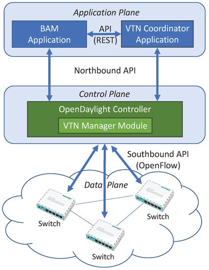
Figure 1.
The proposed SDN-based network architecture.
Concurrent IoT applications may have diverse QoS requirements, which may be difficult to satisfy on the same network. For example, let us assume that there is an IoT network of autonomous cars. If the cars’ high definition video sensors and the control systems are on the same network, a congestion in the network due to video transmission may disrupt control communication and result in a car accident [10]. Network slicing solves this problem by creating separate logical networks upon a shared physical network. By logically separating their networks, network slicing can facilitate IoT services with diverse requirements on the same physical infrastructure while satisfying their QoS requirements. Moreover, network slicing allows the isolation of IoT device communications for security [11]. Our framework supports network slicing through SDN, so it can improve the QoS and security of IoT networks.
To create and manage the network slices on the physical network, we use the SDN-based virtual tenant network (VTN) feature. The VTN feature allows the setting up of multiple isolated virtual networks with different routing tables at each network slice, so it is possible to do slice-specific traffic engineering for optimizing QoS. Moreover, it allows limiting the data traffic to a different subset of links at each VNT slice. The physical links that are not used by any virtual links in slices can be disabled for decreasing the power consumption, which is important for some networks using low-power IoT devices.
The VTN feature is composed of the VTN coordinator application and VTN manager. The VTN coordinator is an external SDN application that realizes VTN provisioning and provides a REST interface to enable the use of OpenDaylight VTN virtualization. The VTN manager is an OpenDaylight module that interacts with other modules to implement the components of the VTN model. The VTN coordinator application translates the REST API commands from other applications and sends them to the VTN manager. The VTN coordinator supports coordinating multiple VTN managers, so virtual networks spanning across multiple OpenDaylight controllers can be created and managed by a single VTN coordinator. By using the REST API of the VTN coordinator, our application can set up and modify the network slices.
Due to the large number of source-destination pairs and large number of flows, estimating the traffic matrix precisely in a large IP network is extremely difficult, and it has been recognized as a challenging research problem [23]. Compared to traditional IP networks, SDN has some important advantages for traffic measurements. First of all, the SDN controller has a global view of the SDN network topology. Second, the SDN controller can collect flow-level and port (link)-level statistics from the SDN switches by using a southbound protocol like OpenFlow [42]. However, the traffic matrix estimation is still challenging even with SDN. Instead of trying to estimate the overall traffic matrix from flow statistics in such networks, our BAM-based traffic engineering framework tries to identify the traffic pattern by using only the utilization level of a set of edge links. The number of ports in a network is usually much lower than the number of flows, so transmitting the link utilization statistics requires much less bandwidth. The OpenDaylight controller automatically collects the port statistics of switches every three seconds by OpenFlow and provides the port statistics to the SDN applications via the northbound REST API.
Initially, a list of possible traffic patterns is given as Bayesian attractors to our application. The BAM assigns stochastic variables to these attractors that indicate the confidence level of each attractor. Together with the traffic patterns, pre-calculated network slice topologies and routing tables optimized for each traffic pattern are given to our application by its API. Our SDN application periodically receives the utilization statistics of a set of edge links from the OpenDaylight controller. The BAM updates the confidence level of attractors each time when there is a new observation of these fluctuating and noisy statistics. By comparing these confidence levels, the application tries to identify the current traffic pattern from a list of stored patterns. In the case of a change in the identified traffic pattern, the application sends the network slice VNT configuration and the routing tables in each network slice, which were pre-optimized for the identified traffic, to the VTN coordinator application via the REST API. The VTN coordinator application translates the requested configuration and sends it to the VTN manager module in the corresponding OpenDaylight controller, which controls the SDN network that is to be modified. The VTN manager module updates the configuration of the OpenDaylight controller for setting up the new logical network. Finally, the OpenDaylight controller pushes down the changes to the switches by the southbound OpenFlow API. In case of a change in the traffic patterns to be identified, the new list of traffic patterns can be given to the application, which restarts the BAM. As BAM is an online algorithm and it does not require training, BAM can identify the new patterns after getting a few samples of utilization statistics.
5. The Testbed
To show that our SDN framework can identify the changing traffic patterns and increase the QoS of an IoT network by immediately applying a pre-calculated network configuration optimized to the new pattern, we implemented our framework as an SDN application on OpenDaylight and tested it on an SDN testbed. A photo of the testbed is shown in Figure 2. A plot of the testbed topology is shown in Figure 3. In the testbed, there were 9 SDN core switches, where eight were MikroTik RouterBOARD 750Gr3 switches with 1 Gbps ports, and the other one was a Pica8 SDN switch with 1 Gbps and 10 Gbps ports. A Spirent hardware traffic generator was used for generating realistic traffic and analyzing the traffic statistics like packet drop rate and delays. The Spirent hardware traffic generator sent the generated traffic to a non-SDN Dell switch through a 10 Gbps optical link. The Dell switch distributed the generated traffic to MikroTik switches. The Pica8 switch forwarded the collected traffic to the sink of the Spirent traffic generator through a 10 Gbps optical link. To make the MikroTik switches SDN-capable, their firmware was replaced with an OpenWRT embedded operating system and Open vSwitch switching software. Our SDN application, the Spirent TestCenter application, the VTN Coordinator application, and the OpenDaylight SDN controller were installed on a computer that communicates with the SDN switches and the traffic generator via a separate network for the out-of-band control of the testbed.
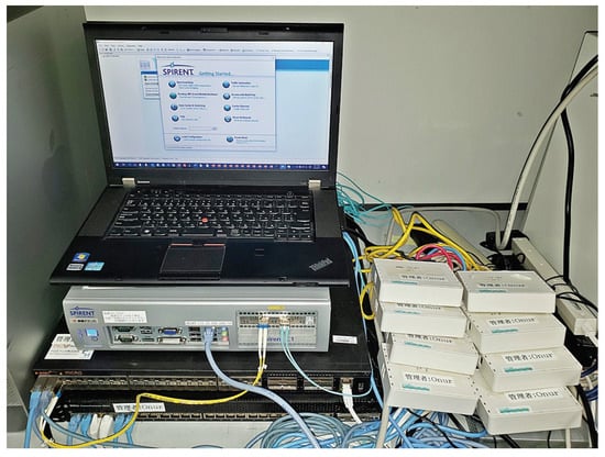
Figure 2.
A photo of the testbed.
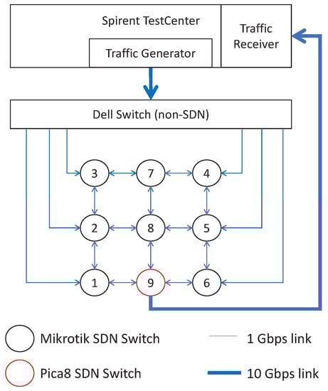
Figure 3.
The topology of the testbed.
6. The Experiment
In the experiment, we emulated an IoT network of a crowd surveillance system around a building using two different types of video sensors generating surveillance data, e.g., visible-light video, infrared video etc. Recently, IoT-based crowd surveillance systems have become popular due to their cost effectiveness in many applications like public safety (against terrorist attacks, demonstrations, natural disasters, etc.) and smart cities [43,44,45,46]. The IoT network topology and the initial traffic rate of sensors is shown in Figure 4. In the IoT network, there were six dumb edge nodes, each carrying two types of sensors, and nine SDN core switches with the same numbering as in Figure 3. The dumb edge nodes were not SDN-capable. The Spirent hardware traffic generator generated realistic sensor traffic by emulating twelve sensors, where six of them are type 1 sensors, and six of them are type 2 sensors. Each sensor generated and sent one-way traffic to an IoT gateway node that forwards the data generated in the IoT domain to the wide-area network (WAN). The IoT gateway node was emulated by the traffic receiver of Spirent TestCenter, which measured the network statistics from the arriving packets.
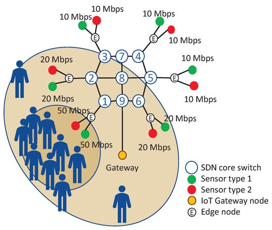
Figure 4.
The IoT network topology and the initial traffic rate of sensors when the crowd was close to the edge of core node 1.
In the experiment scenario, there was a gathering of a crowd around a building. The sensors of the crowd surveillance system were placed at six places around the building. The bitrate of traffic generated by a sensor increased with the number of people in the vicinity of the sensor due to increased activity. For simplicity, we set the generated data rate of both sensor types to be equal to each other in the experiment. Due to the SDN packet processing speed limitations of MikroTik switches, we could not fully utilize the links to cause link congestion. We chose the sensor traffic rates to limit the traffic on the core links to 200 Mbps to prevent crashing of MikroTik switches due to CPU over-utilization. Each of the sensors that were closest to the center of the crowd, like the sensors connected to the edge node of core node 1 in Figure 4, identified fast-paced movement of many people so they generated traffic using an ABR video codec with a high bitrate of 50 Mbps to keep the video quality high. The sensors that were in the vicinity but not so close to the center of the crowd, like the sensors connected to the edge node of core nodes 2 and 6 in Figure 4, identified less movement, so they used a codec that generated 20 Mbps ABR traffic. The sensors that were far away from the crowd did not identify much movement, so they used a codec that generated 10 Mbps ABR traffic.
There were six edge nodes in the network, so we selected six possible traffic patterns where the crowd is closest to one of the six edge nodes. In the experiment, we tested a scenario where a crowd moves back and forth between the edge sensors of core node 1 as in Figure 4 and the edge sensors of core node 5 as shown in Figure 5. The sensors generated random traffic with a lognormal size distribution with a mean as in Figure 4 and Figure 5. OpenDaylight fetched traffic rate information from SDN core devices by OpenFlow every three seconds, and our application fetched these edge link traffic rate statistics from OpenDaylight via the northbound API. Our application tried to identify the latest traffic matrix by using the BAM.
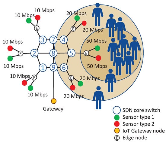
Figure 5.
The traffic rate of sensors after the crowd moved to the edge of core node 5.
The average traffic rate on the edge links in each scenario was stored as a BAM attractor in the application. For example, the BAM attractor of the pattern shown in Figure 4, when the crowd is around the edge of core node 1, was simply an array [100 40 20 20 20 40] in terms of Mbps, where the array index is the core node number where the edge link was connected. As the traffic is entering the SDN network through six core routers and the IoT traffic in the experiment was one-way, the size of each BAM attractor was . It is possible to add more traffic patterns as attractors, but we limited the number of traffic patterns to six in this experiment for a more clear presentation of attractor dynamics.
For each of the selected traffic patterns, we pre-computed the VNT configurations and routing tables of the network slices optimized for the traffic scenario and stored them in our application along with the corresponding BAM attractor. As an example, the VNT configuration of network slices optimized for the traffic pattern in Figure 4 is shown in Figure 6a. VNT configuration of another pattern in Figure 5 is shown in Figure 6b. In the network, the traffic of sensor type 1 was assigned to network slice 1, and the traffic of sensor type 2 was assigned to network slice 2. To minimize the maximum link utilization and maximize the power efficiency in the experiment, we optimized the VNT configuration in two steps. In the first step, for a selected traffic pattern, the set of routing tables at each network slice that minimizes the maximum link utilization in the physical network was found. Then, among the solutions of the first step, a solution that uses the minimum number of physical links when routing the aggregate traffic is selected to minimize the power consumption as the links that are unused in all slices can be set to idle. For example, four physical links in Figure 6a were set to idle because none of the VNTs used them. While VNT was the same in both slices in Figure 6a, the slices had different routing tables to minimize the overall maximum link utilization of the physical network. For example, the traffic from the edge of core node 1 to the edge of core node 9 followed the path 1→9 on slice 1, while the traffic between the same edge nodes followed the path 1→2→8→9 on slice 2 as shown with arrows. The VNTs on slices may also differ depending on the placement of sensors and the traffic matrix on each slide.
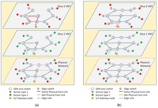
Figure 6.
The VNTs in the network slices and the active/idle link configuration in the physical topology optimized for the initial traffic matrix when the crowd was close to (a) the edge of core node 1 and (b) the edge of core node 5.
The edge link traffic rate statistics fetched by our application via the northbound of SDN controller in the experiment are shown in Figure 7. The edge links are numbered according to the number of the core node that they are connected to. The traffic of sensors started in the first 3 s. The first edge link traffic statistic were fetched at time 3 s. Initially, the crowd was around the sensors connected to core 1, so those sensors were producing the highest traffic and the edge link 1 had the highest link utilization as seen in Figure 4. Figure 8 shows the traffic rate on the link from core node 6 to core node 9 and the link from core node 1 to core node 9, which are the most congested core links in the network. Initially, the network configuration was not optimized for this traffic pattern, so the link from core node 1 to core node 9 started to carry high amount of traffic at time 10 s. The BAM algorithm in our application tried to identify the traffic pattern by using the traffic rate statistics of the edge links. Each time a new observation of statistics was fetched, BAM updated the confidence level of the attractors. The confidence level of the attractors calculated by BAM during the experiment is shown in Figure 9. Initially, the confidence level of all attractors were zero. After getting only two traffic statistics, the confidence level of attractor 1 became the highest and the confidence difference between the highest and the second highest attractors passed the threshold set to 0.5, so attractor 1 was correctly identified as the new state. The attractor identified as the current traffic pattern by BAM is shown in Figure 10. The attractors number 1 and number 5 denote the traffic patterns when the crowd is around the edge sensors of core node 1 and core node 5, respectively. The time when BAM identified a new traffic pattern is denoted by IT (Identified Traffic) and shown with blue dashed lines in the experiment results.
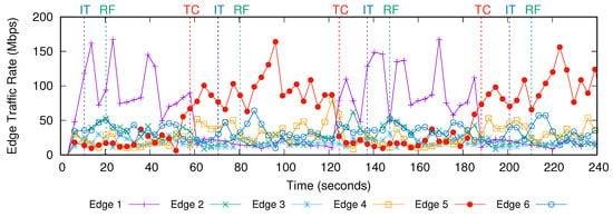
Figure 7.
The edge link traffic rate statistics fetched by our application from OpenDaylight.
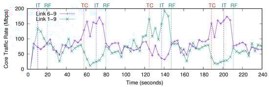
Figure 8.
The traffic rate on the links from core node 6 to core node 9 and core node 1 to core node 9.
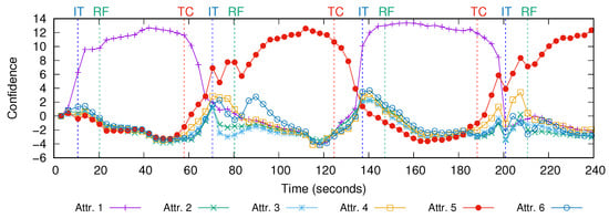
Figure 9.
The confidence level of the attractors.
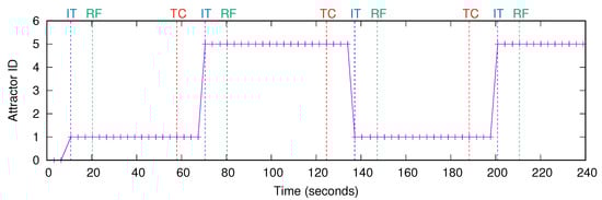
Figure 10.
The identified traffic pattern by the decision algorithm.
After identifying the new traffic pattern, our SDN application sent the VNT and routing table configuration optimized for traffic pattern 1 to the VTN coordinator by using its REST API. The VTN coordinator translated the configuration request of the application, updated its VTN configuration database, and sent it the OpenDaylight controller via the VTN manager. Finally, the OpenDaylight controller applied the new configuration to the SDN network by updating the flow tables of the switches by OpenFlow. This network reconfiguration process took around 10 s and finished at time 20 s, which is denoted by RF (Reconfiguration Finished) and shown with green dashed lines in the experiment results. After RF, the network started to run using a configuration optimized for this identified traffic matrix, so the maximum link utilization in the network decreased as seen in Figure 8.
Later, the crowd moved near the edge sensors of core node 5 and the traffic rate of the sensors changed as shown in Figure 5. As a result, there was an abrupt change in the traffic of edge and core links at time 58 s, which is denoted by TC (Traffic Changed) and shown with red dashed lines in the experiment results. The traffic rate on the edge link 5 became the highest as seen in Figure 7. The utilization of core link from node 9 to node 1 increased around two times as seen in Figure 8 because the network configuration was not optimized for the new traffic matrix. After the traffic change, the confidence level of attractor 1 started to decrease and the confidence level of attractor 5 started to increase as seen in Figure 9. At time 70 s, the confidence of attractor 5 passed that of attractor 1, and the BAM identified the traffic pattern of attractor 5 as the new traffic pattern as seen in Figure 10. Therefore BAM required fetching edge link traffic statistics only 5 times to identify the new traffic matrix. After identifying the new traffic pattern, our SDN application reconfigured the network to a configuration optimized for the identified traffic matrix, which took around 10 s and finished at time 80 s. After the reconfiguration finished, the maximum link utilization in the network decreased by two times.
We repeated the traffic changes by moving the crowd to near the edge sensors of core node 1 at time 125 and then core node 5 at time 188 s. Again, BAM correctly identified the new traffic matrices after 5 iterations of fetching traffic statistics and our framework decreased the maximum link utilization by two times by reconfiguring the network via SDN.
Our SDN application was run on a laptop with an Intel i7-3820QM CPU. Even though our BAM implementation was not so optimized, the application used less than 10% of the single core of the laptop CPU produced in year 2012, which can be considered as a low CPU usage. Due to the budget constraints we couldn’t set up a bigger testbed and we couldn’t find a reference in the literature that evaluates the processing requirements of BAM, so the processing requirements of BAM on larger networks is not clear. In case the computation cost of the BAM becomes high, it may be decreased by replacing UKF with EKF, which is known to have a lower computational cost than UKF [47,48], in the BAM implementation. Bitzer et al. [8] says that they used the UKF in the BAM, because it provides a suitable tradeoff between the precision and computational efficiency. However, Bitzer et al. [8] states that EKF, which is faster but less precise than UKF, can also be used in the BAM.
7. Conclusions
In this paper, we presented a framework based on the Bayesian attractor model and SDN for optimizing the IoT networks that exhibit a limited number of traffic patterns. We implemented the framework as an SDN application and investigated its feasibility on an SDN testbed. The experiment results showed that our application can identify the traffic pattern with a few observations of edge link traffic statistics, which should be fast enough for most networks, and can apply an optimized network configuration for the identified traffic pattern by SDN. To the best of our knowledge, ours is the first work that tries to directly identify a traffic matrix from a known list of traffic matrices using only link utilization statistics, so we could not find another algorithm in the literature for direct comparison in the experiments. There may be even faster identification algorithms, but using the BAM for the identification has important merits like the BAM is an online algorithm and it does not require training or partial measurements of traffic matrix. Moreover, the BAM-based application had a low CPU utilization in the experiment. Furthermore, the BAM may open the way towards more autonomous networks by adding a more human-like artificial intelligence to the network. We showed that our application can apply network slicing-based traffic engineering for optimizing the utilization and power efficiency of core links. As a possible limitation, the CPU requirements and the identification time may increase with increasing number of nodes and limit the size of the controllable network. For future work, we will set up a bigger testbed to evaluate the performance of the framework on large networks. Moreover, we will work on adding support for using other SDN controller software platforms like ONOS. As other areas of application, the framework may be also applied to other types of networks like cellular networks. We will investigate its applicability to other networks in our future work.
Author Contributions
Conceptualization, O.A., S.A. and M.M.; methodology, O.A., S.A. and M.M.; software, O.A.; validation, O.A.; formal analysis, O.A., S.A. and M.M.; investigation, O.A.; resources, O.A. and S.A.; data curation, O.A.; writing—original draft preparation, O.A.; writing—review and editing, O.A.; visualization, O.A.; supervision, S.A. and M.M.; project administration, S.A. and M.M.; funding acquisition, S.A. and M.M. All authors have read and agreed to the published version of the manuscript.
Funding
This research and development work was supported by Ministry of Internal Affairs and Communications of Japan.
Conflicts of Interest
The authors declare no conflict of interest. The funders had no role in the design of the study; in the collection, analyses, or interpretation of data; in the writing of the manuscript, or in the decision to publish the results.
References
- Jain, R.; Paul, S. Network virtualization and software defined networking for cloud computing: A survey. IEEE Commun. Mag. 2013, 51, 24–31. [Google Scholar] [CrossRef]
- Xie, J.; Yu, F.R.; Huang, T.; Xie, R.; Liu, J.; Wang, C.; Liu, Y. A Survey of machine learning techniques applied to software defined networking (SDN): Research issues and challenges. IEEE Commun. Surv. Tutor. 2019, 21, 393–430. [Google Scholar] [CrossRef]
- Latah, M.; Toker, L. Artificial intelligence enabled software-defined networking: A comprehensive overview. IET Netw. 2019, 8, 79–99. [Google Scholar] [CrossRef]
- Queiroz, W.; Capretz, M.A.; Dantas, M. An approach for SDN traffic monitoring based on big data techniques. J. Netw. Comput. Appl. 2019, 131, 28–39. [Google Scholar] [CrossRef]
- Hsu, C.Y.; Tsai, P.W.; Chou, H.Y.; Luo, M.Y.; Yang, C.S. A flow-based method to measure traffic statistics in software defined network. In Proceedings of the Asia-Pacific Advanced Network, Bandung, Indonesia, 20–24 January 2014; Volume 38, p. 19. [Google Scholar] [CrossRef]
- Li, M.; Chen, C.; Hua, C.; Guan, X. CFlow: A learning-based compressive flow statistics collection scheme for SDNs. In Proceedings of the 2019 IEEE International Conference on Communications (ICC), Shanghai, China, 20–24 May 2019; pp. 1–6. [Google Scholar] [CrossRef]
- Malboubi, M.; Peng, S.M.; Sharma, P.; Chuah, C.N. A learning-based measurement framework for traffic matrix inference in software defined networks. Comput. Electr. Eng. 2018, 66, 369–387. [Google Scholar] [CrossRef]
- Bitzer, S.; Bruineberg, J.; Kiebel, S.J. A Bayesian attractor model for perceptual decision making. PLoS Comput. Biol. 2015, 11, e1004442. [Google Scholar] [CrossRef]
- Ohba, T.; Arakawa, S.; Murata, M. Bayesian-based virtual network reconfiguration for dynamic optical networks. IEEE/OSA J. Opt. Commun. Netw. 2018, 10, 440–450. [Google Scholar] [CrossRef]
- Kafle, V.P.; Fukushima, Y.; Martinez-Julia, P.; Miyazawa, T.; Harai, H. Adaptive virtual network slices for diverse IoT services. IEEE Commun. Stand. Mag. 2018, 2, 33–41. [Google Scholar] [CrossRef]
- Esaki, H.; Nakamura, R. Overlaying and slicing for IoT era based on Internet’s end-to-end discipline. In Proceedings of the 2017 IEEE International Symposium on Local and Metropolitan Area Networks (LANMAN), Osaka, Japan, 12–14 June 2017; pp. 1–6. [Google Scholar] [CrossRef]
- Vardi, Y. Network tomography: Estimating source-destination traffic intensities from link data. J. Am. Stat. Assoc. 1996, 91, 365–377. [Google Scholar] [CrossRef]
- Tebaldi, C.; West, M. Bayesian inference on network traffic using link count data. J. Am. Stat. Assoc. 1998, 93, 557–573. [Google Scholar] [CrossRef]
- Cao, J.; Davis, D.; Wiel, S.V.; Yu, B. Time-varying network tomography: Router link data. J. Am. Stat. Assoc. 2000, 95, 1063–1075. [Google Scholar] [CrossRef]
- Medina, A.; Taft, N.; Salamatian, K.; Bhattacharyya, S.; Diot, C. Traffic matrix estimation: Existing techniques and new directions. In Proceedings of the ACM SIGCOMM 2002 Conference on Applications, Technologies, Architectures, and Protocols for Computer Communication, Pittsburgh, PA, USA, 19–23 August 2002; Volume 32, pp. 161–174. [Google Scholar] [CrossRef]
- Roughan, M.; Greenberg, A.; Kalmanek, C.; Rumsewicz, M.; Yates, J.; Zhang, Y. Experience in measuring backbone traffic variability: Models, metrics, measurements and meaning. In Proceedings of the 2nd ACM SIGCOMM Workshop on Internet Measurment, Marseille, France, 6–8 November 2002; Association for Computing Machinery: New York, NY, USA, 2002; pp. 91–92. [Google Scholar] [CrossRef]
- Zhang, Y.; Roughan, M.; Duffield, N.; Greenberg, A. Fast accurate computation of large-scale IP traffic matrices from link loads. In Proceedings of the International Conference on Measurements and Modeling of Computer Systems, SIGMETRICS 2003, San Diego, CA, USA, 9–14 June 2003; pp. 206–217. [Google Scholar] [CrossRef]
- Eum, S.; Murphy, J.; Harris, R.J. A failure analysis of the tomogravity and EM methods. In Proceedings of the TENCON 2005—2005 IEEE Region 10 Conference, Melbourne, Australia, 21–24 November 2005; pp. 1–6. [Google Scholar]
- Lakhina, A.; Papagiannaki, K.; Crovella, M.; Diot, C.; Kolaczyk, E.D.; Taft, N. Structural analysis of network traffic flows. In Proceedings of the Joint International Conference on Measurement and Modeling of Computer Systems, New York, NY, USA, 12–16 June 2004; Volume 32, pp. 61–72. [Google Scholar] [CrossRef]
- Soule, A.; Salamatian, K.; Nucci, A.; Taft, N. Traffic matrix tracking using Kalman filters. In Proceedings of the 2005 ACM SIGMETRICS International Conference on Measurement and Modeling of Computer Systems, Banff, AB, Canada, 6–10 June 2005; Volume 33, pp. 24–31. [Google Scholar] [CrossRef]
- Papagiannaki, K.; Taft, N.; Lakhina, A. A distributed approach to measure IP traffic matrices. In Proceedings of the 2004 ACM SIGCOMM Internet Measurement Conference, Taormina, Italy, 25–27 October 2004; pp. 161–174. [Google Scholar] [CrossRef]
- Soule, A.; Lakhina, A.; Taft, N.; Papagiannaki, K.; Salamatian, K.; Nucci, A.; Crovella, M.; Diot, C. Traffic matrices: Balancing measurements, inference and modeling. In Proceedings of the 2005 ACM SIGMETRICS International Conference on Measurement and Modeling of Computer Systems, Banff, AB, Canada, 6–10 June 2005; Volume 33, pp. 362–373. [Google Scholar] [CrossRef]
- Zhao, Q.; Ge, Z.; Wang, J.; Xu, J. Robust traffic matrix estimation with imperfect information: Making use of multiple data sources. In Proceedings of the Joint International Conference on Measurement and Modeling of Computer Systems, Saint Malo, France, 26–30 June 2006; Volume 34, pp. 133–144. [Google Scholar] [CrossRef]
- Nie, L.; Wang, H.; Jiang, X.; Guo, Y.; Li, S. Traffic measurement optimization based on reinforcement learning in large-scale ITS-oriented backbone networks. IEEE Access 2020, 8, 36988–36996. [Google Scholar] [CrossRef]
- Kumar, A.; Vidyapu, S.; Saradhi, V.V.; Tamarapalli, V. A multi-view subspace learning approach to Internet traffic matrix estimation. IEEE Trans. Netw. Serv. Manag. 2020, 17, 1282–1293. [Google Scholar] [CrossRef]
- Tootoonchian, A.; Ghobadi, M.; Ganjali, Y. OpenTM: Traffic Matrix Estimator for OpenFlow Networks. In Passive and Active Measurement; Krishnamurthy, A., Plattner, B., Eds.; Springer: Berlin/Heidelberg, Germany, 2010; pp. 201–210. [Google Scholar]
- Yu, Y.; Qian, C.; Li, X. Distributed and collaborative traffic monitoring in software defined networks. In Proceedings of the Third Workshop on Hot Topics in Software Defined Networking, Chicago, IL, USA, 17–22 August 2014; Association for Computing Machinery: New York, NY, USA, 2014; pp. 85–90. [Google Scholar] [CrossRef]
- Malboubi, M.; Wang, L.; Chuah, C.; Sharma, P. Intelligent SDN based traffic (de)aggregation and measurement paradigm (iSTAMP). In Proceedings of the IEEE INFOCOM 2014—IEEE Conference on Computer Communications, Toronto, ON, Canada, 27 April–2 May 2014; pp. 934–942. [Google Scholar]
- Gong, Y.; Wang, X.; Malboubi, M.; Wang, S.; Xu, S.; Chuah, C.N. Towards accurate online traffic matrix estimation in software-defined networks. In Proceedings of the 1st ACM SIGCOMM Symposium on Software Defined Networking Research, Santa Clara, CA, USA, 17–18 June 2015; Association for Computing Machinery: New York, NY, USA, 2015. [Google Scholar] [CrossRef]
- Liu, C.; Malboubi, A.; Chuah, C. OpenMeasure: Adaptive flow measurement inference with online learning in SDN. In Proceedings of the 2016 IEEE Conference on Computer Communications Workshops (INFOCOM WKSHPS), San Francisco, CA, USA, 10–14 April 2016; pp. 47–52. [Google Scholar]
- Polverini, M.; Baiocchi, A.; Cianfrani, A.; Iacovazzi, A.; Listanti, M. The power of SDN to improve the estimation of the ISP traffic matrix through the flow spread concept. IEEE J. Sel. Areas Commun. 2016, 34, 1904–1913. [Google Scholar] [CrossRef]
- Tian, Y.; Chen, W.; Lea, C. An SDN-based traffic matrix estimation framework. IEEE Trans. Netw. Serv. Manag. 2018, 15, 1435–1445. [Google Scholar] [CrossRef]
- Jiang, D.; Hu, G. Large-scale IP traffic matrix estimation based on backpropagation neural network. In Proceedings of the 2008 First International Conference on Intelligent Networks and Intelligent Systems, Wuhan, China, 1–3 November 2008; pp. 229–232. [Google Scholar]
- Casas, P.; Vaton, S. On the use of random neural networks for traffic matrix estimation in large-scale IP networks. In Proceedings of the 6th International Wireless Communications and Mobile Computing Conference, Caen, France, 28 June–2 July 2010; Association for Computing Machinery: New York, NY, USA, 2010; pp. 326–330. [Google Scholar] [CrossRef]
- Zhou, H.; Tan, L.; Zeng, Q.; Wu, C. Traffic matrix estimation: A neural network approach with extended input and expectation maximization iteration. J. Netw. Comput. Appl. 2016, 60, 220–232. [Google Scholar] [CrossRef]
- Nie, L.; Jiang, D.; Guo, L.; Yu, S. Traffic matrix prediction and estimation based on deep learning in large-scale IP backbone networks. J. Netw. Comput. Appl. 2016, 76, 16–22. [Google Scholar] [CrossRef]
- Emami, M.; Akbari, R.; Javidan, R.; Zamani, A. A new approach for traffic matrix estimation in high load computer networks based on graph embedding and convolutional neural network. Trans. Emerg. Telecommun. Technol. 2019, 30, e3604. [Google Scholar] [CrossRef]
- Huo, L.; Jiang, D.; Lv, Z.; Singh, S. An intelligent optimization-based traffic information acquirement approach to software-defined networking. Comput. Intell. 2020, 36, 151–171. [Google Scholar] [CrossRef]
- Nie, L.; Li, Y.; Kong, X. Spatio-temporal network traffic estimation and anomaly detection based on convolutional neural network in vehicular ad-hoc networks. IEEE Access 2018, 6, 40168–40176. [Google Scholar] [CrossRef]
- Hu, Z.; Qiao, Y.; Luo, J. ATME: Accurate traffic matrix estimation in both public and private datacenter networks. IEEE Trans. Cloud Comput. 2018, 6, 60–73. [Google Scholar] [CrossRef]
- Wan, E.A.; Van Der Merwe, R. The unscented Kalman filter for nonlinear estimation. In Proceedings of the IEEE 2000 Adaptive Systems for Signal Processing, Communications, and Control Symposium, Lake Louise, AB, Canada, 4 October 2000; pp. 153–158. [Google Scholar] [CrossRef]
- McKeown, N.; Anderson, T.; Balakrishnan, H.; Parulkar, G.; Peterson, L.; Rexford, J.; Shenker, S.; Turner, J. OpenFlow: Enabling innovation in campus networks. In Proceedings of the SIGCOMM 2018, Seattle, WA, USA, 17–22 August 2008; Volume 38, pp. 69–74. [Google Scholar] [CrossRef]
- Pathan, A.S.K. Crowd Assisted Networking and Computing; CRC Press: Boca Raton, FL, USA, 2018. [Google Scholar]
- Motlagh, N.H.; Bagaa, M.; Taleb, T. UAV-based IoT platform: A crowd surveillance use case. IEEE Commun. Mag. 2017, 55, 128–134. [Google Scholar] [CrossRef]
- Memos, V.A.; Psannis, K.E.; Ishibashi, Y.; Kim, B.G.; Gupta, B. An efficient algorithm for media-based surveillance system (EAMSuS) in IoT smart city framework. Future Gener. Comput. Syst. 2018, 83, 619–628. [Google Scholar] [CrossRef]
- Gribaudo, M.; Iacono, M.; Levis, A.H. An IoT-based monitoring approach for cultural heritage sites: The Matera case. Concurr. Comput. Pract. Exp. 2017, 29, e4153. [Google Scholar] [CrossRef]
- St-Pierre, M.; Gingras, D. Comparison between the unscented Kalman filter and the extended Kalman filter for the position estimation module of an integrated navigation information system. In Proceedings of the 2004 IEEE Intelligent Vehicles Symposium, Parma, Italy, 14–17 June 2004; pp. 831–835. [Google Scholar]
- Fiorenzani, T.; Manes, C.; Oriolo, G.; Peliti, P. Comparative Study of Unscented Kalman Filter and Extended Kalman Filter for Position/attitude Estimation in Unmanned Aerial Vehicles; Technical Report; The Institute for Systems Analysis and Computer Science: Rome, Italy, 2008. [Google Scholar]
© 2020 by the authors. Licensee MDPI, Basel, Switzerland. This article is an open access article distributed under the terms and conditions of the Creative Commons Attribution (CC BY) license (http://creativecommons.org/licenses/by/4.0/).