Abstract
In real engineering scenarios, it is difficult to collect adequate cases with faulty conditions to train an intelligent diagnosis system. To alleviate the problem of limited fault data, this paper proposes a fault diagnosis method combining a generative adversarial network (GAN) and stacked denoising auto-encoder (SDAE). The GAN approach augments the limited real measured data, especially in faulty conditions. The generated data are then transformed into the SDAE fault diagnosis model. The GAN-SDAE approach improves the accuracy of the fault diagnosis from the vibration signals, especially when the measured samples are few. The usefulness of this method is assessed through two condition-monitoring cases: one is a classic bearing example and the other is a more general gear failure. The results demonstrate that diagnosis accuracy for both cases is above 90% for various working conditions, and the GAN-SDAE system is stable.
1. Introduction
Fault diagnosis is necessary for mechanical equipment in modern industries [1,2,3]. Through condition monitoring, the signals of various sensors are extracted and analyzed for fault diagnosis. Because of the inconstancy and enrichment of the response signals under harsh operating conditions, it is difficult to identify the failure mode of mechanical systems.
Deep learning algorithms for diagnosing machinery faults have become prevalent owing to their robustness and capacity for adaptation. Deep architectures of computational layers and neurons are the foundation of deep learning. Roozbeh et al. [4] proposed a semi-supervised and deep ladder network (SSDLN); with few labeled samples, the model is trained through a high-dimensional feature space to diagnose gear failures. Zhang et al. [5] presented a novel unsupervised learning algorithm based on the generalized norm of the feature matrix for intelligent fault diagnosis. The feature sparsity was successfully measured by optimizing the objective function. However, in real engineering scenarios, it is difficult to identify useful details in the recorded fault signal. Therefore, it is necessary to reduce the feature dimensions. Khare et al. [6] proposed a spider monkey optimization (SMO)-based deep neural network (DNN) model. Compared to the classic DNN model, the SMO-DNN achieved a dimensionality reduction and accurate classification. As another classic deep learning model, the deep belief network conducts information fusion through data reduction [7]. Wang et al. [8] presented an unsupervised fault-diagnosis model using the sparse-filtering algorithm. The model uses the learned fault features to classify different fault types.
Current deep learning is inherently challenged by an unstable network structure. It is necessary to analyze the robust stability of deep neural networks [9]. Compared to other deep learning methods, the sparse denoising auto-encode (SDAE) model is established by a series of auto-encoders and has a stable deep network structure with a layer-by-layer nature [10]. The SDAE is widely used in fault diagnosis of rotating machinery. Typical examples are gears and bearings [11,12]. Another problem of deep learning is that many training samples are required. Deep learning models are traditionally big data driven and an obvious lack of sufficient training affects the accuracy of the model [13]. Based on a relatively small dataset, Sulikowski et al. [14] presented a deep learning-enhanced framework that had a satisfactory accuracy. However, in practice, there are very few fault samples affected by cost. In traditional mathematical statistics, the definition of small sample data is that of samples of size n ≤ 30 [15]. Obviously, most of the fault samples are small sample data, which lead to limitations in the data [16]. This data limitation results in poor model performance, as shown in Figure 1 [17]. The deep learning model of fault diagnosis is trained by a few training samples. Given the limited fault data, the model training is often insufficient, resulting in an inaccurate fault diagnosis. Therefore, data limitation is a huge challenge for deep-learning model training. So, we propose the generative adversarial network (GAN) data-augmentation to effectively solve the data-limitation problem. In the current era of fierce artificial intelligence, GAN can productively solve the problem of small-sample data with insufficient data volumes. Based on artificial intelligence theory, GAN provides enough data for deep learning training.
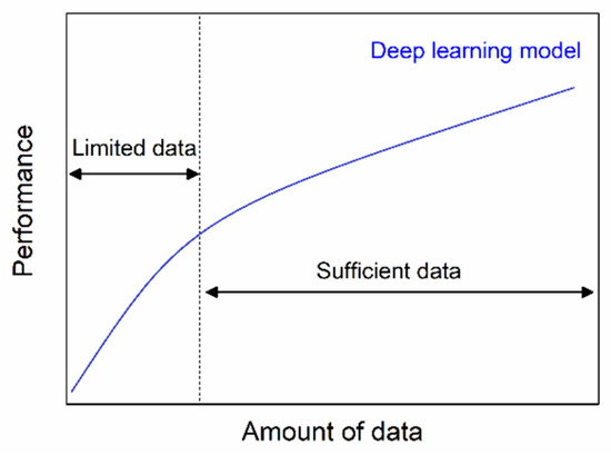
Figure 1.
The relationship between performance and data volume.
The GAN is a data-augmentation model proposed by Goodfellow [18]. It has been proverbially applicable to image processing. Wang et al. [19] proposed a new method called 3D GAN to calculate the full-dose images with low-dose ones. The conclusion showed that the 3D GAN method outperformed the benchmark methods. Similarly, Ma et al. [20] presented a GAN method to fuse the images with different resolutions. The results demonstrated that the strategy generated clear, clean fused images, without the noise caused by up-sampling of infrared information. In the GAN approach, the joint distribution of latent representations was sought by adversarial layers [21,22]. After adversarial learning, the trained latent representations were well-aligned to explain the co-occurrence configurations of the fused images.
Ghorban et al. [23] presented a multichannel GAN for generating traffic signs. In contrast to other existing approaches, the proposed method processed multiple channels with different textures and resolutions. Similarly, the principle of GAN has been applied to fault diagnosis. Usually, the testing data from different machine-fault conditions are unavailable for training; however, deep generative neural networks can provide reliable diagnoses by artificially generating training samples [24]. In practical working conditions with data-acquisition equipment, the achievable fault data are really limited. Furthermore, the problem of fault types being unevenly distributed also restricts the diagnostic accuracy. To solve these problems, Mao et al. [25] presented an imbalanced fault diagnosis method using GAN. Moreover, a detailed comparative study is provided in this paper. Considering the mode collapse of GAN, Wen et al. [26] presented a deep learning method to identify different failure modes of gears. However, the study did not consider the robustness of the model under different operating and faulty conditions, such as different workloads and fault sizes. In addition, the quality of the generated data needs to be analyzed. Mode collapse is another challenge of the GAN model [27]. A novel GAN model with a gradient penalty term was designed to avoid model collapse, thereby ensuring model performance.
This paper combines the results of deep learning network applications in other fields with the characteristics of a vibration signal. The SDAE [28] was used to mine implied feature information from complex vibration signals. Compared to the prime deep learning for complex fault diagnosis, the superiority of SDAE is that it uses the depth structure to mine the essential information. In addition, SDAE is robust, which reduces the influence of noise on the recognition results to enhance their accuracy. Furthermore, GAN solves the problem of insufficient SDAE training samples.
We built a novel deep learning system with data augmentation called GAN-SDAE based on waterfall model fusion. For fault diagnosis of complex vibration signals, a single method is not continuously accurate or effective in considering the limitation of the fault samples. Model fusion includes the combination of models that realize different functions and has been widely used in different fault diagnosis fields [29,30]. The fault diagnosis method based on model fusion can complement the advantages of different models and make up for the shortcomings. The GAN model solves the limited fault samples and the SDAE model analyzes the fault types. So, the GAN and SDAE models are integrated and optimized. The GAN-SDAE system for fault diagnosis can greatly improve the ability and accuracy of fault diagnosis. Moreover, the uncertainty of the GAN-SDAE system is analyzed to assure the system stability.
In this paper, we first review the fault diagnosis, which is the basis for building a new model. Secondly, we introduce the GAN data augmentation, and the generated training data are used in the SDAE model training. This process actually constructs the GAN-SDAE system. The accuracy of the GAN-SDAE system is then analyzed and the system is repetitively tested to analyze the system uncertainty. Finally, the usefulness of the proposed system is demonstrated using two examples of bearings and gears. Based on the above introductions, the novelties and highlights of this paper are as follows:
- (1)
- The existing GAN model is improved, by designing a gradient penalty term to avoid model collapse.
- (2)
- Based on waterfall model fusion, the GAN and SDAE models are merged to construct a novel GAN-SDAE system.
- (3)
- The performance and uncertainty of the GAN-SDAE system are fully analyzed.
- (4)
- The GAN-SDAE system is applied to the fault diagnosis of bearings and gears, which proves the effectiveness and versatility of the proposed system.
2. Methodologies
2.1. Fault Diagnosis
Critical machines regularly have permanently installed vibration sensors and transducers, and the acquired vibration signal is used to diagnose the machine for maintenance [31,32]. Many vibrations are directly linked to cyclical events in the machine equipment’s operation, such as rotating shafts gear-teeth. Such events occur often and give a direct indication of the source from the frequency; hence, many powerful diagnostic techniques are usually using frequency analysis.
However, critical industrial machinery always has a complicated configuration and operates under mixed non-stationary modes. The various vibration signals of these machines are complex and are often contaminated by other interference and noises. The collected signals are analyzed with traditional signal-processing methods, such as wavelet analysis and envelope spectrum analysis [33]. More importantly, the traditional fault-diagnosis accuracy is low considering the massive and multiple data. Therefore, it remains a challenge to accurately and intelligently diagnose machine faults using the recorded vibration signals.
2.2. GAN Approach
The GAN approach was inspired by a zero-sum game, and it is able be used to generate many fault signals to achieve data augmentation. The GAN approach consists of two models, namely the generative model (G model) and the discriminant model (D model). Usually, both the G and D models apply a neural network structure, such as the typical multilayer perception network.
The input of the G model is a stochastic noise signal Z = (z1, z2, …, zm) with a data distribution Pz. The output of the G model is the generated signals or samples G(z), with a data distribution Pg that resemble the true distribution Pdata of the original experiment signal. The relationships among the Pz, Pg and Pdata are shown in Figure 2. For example, the generative model can convert a random-noise signal into multiple new signals and transform the data in generated data space to the true data space through the loss.
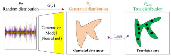
Figure 2.
Relationships among the Pdata. Pz, Pg and Pdata.
The input of the D model is the generated samples G(z) and the true and fault samples X = (x1, x2, …, xn). The output of D model is the probability that the generated fault samples are true samples. The likelihood function L(D, G) of G and D is given by
During the training procedure in GAN, G is first initialized and fixed; then, D is trained by maximizing the loss function in Equation (2). D is upgraded using the stochastic gradient ascending.
The trained D is fixed, and then G is promoted by minimizing the loss function in Equation (3) with the descending stochastic gradient.
The basis of generating vibration fault samples is to ensure their accuracy. Under this premise, the target of D is to recognize the true or false fault samples by exporting the logical value. The G and D models are alternately trained until the GAN model reaches the Nash equilibrium [34]. By combining Equations (2) and (3), the cross-entropy loss of L(D, G) is calculated as follows:
With many peaks, the data distribution of the vibration signals is highly complex and multi-modal. Each peak is called a mode, and each mode represents the concentration of similar failure samples. Mode collapse means that G only exports part of multiple failure modes, and misses other failure modes. In mode collapse, the generated failure samples belongs to a limited set of modes, when G thinks it can fool D by locking a single mode. D eventually finds that the samples in the single mode are fake. However, G is just locked into the single mode, which fundamentally limits the generated samples’ diversity to affect the GAN model performance.
According to the manifold distribution law [35], high-dimensional data of the same category is often concentrated near a low-dimensional manifold. The ideal situation for G is to map the input noise to the manifold where the training data is located, and correspond to the probability distribution of the training data. For example, the probability distribution of a training data set is a simple one-dimensional Gaussian mixture distribution, including two peaks, as shown in Figure 3.
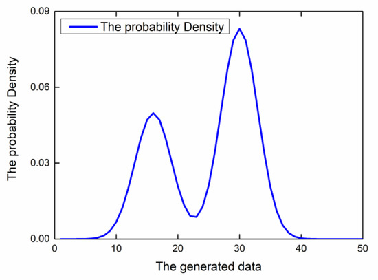
Figure 3.
The one-dimensional Gaussian mixture distribution.
Ideally, the generated samples are as shown in Figure 4 (marked in green). The positions of the generated samples are almost under the two peaks, and the samples conform to the probability distribution of the training set.

Figure 4.
The one-dimensional Gaussian mixture distribution.
However, the ideal situation is almost impossible. In fact, most of the time, there are many generated low-quality samples (marked as red), as shown in Figure 5.
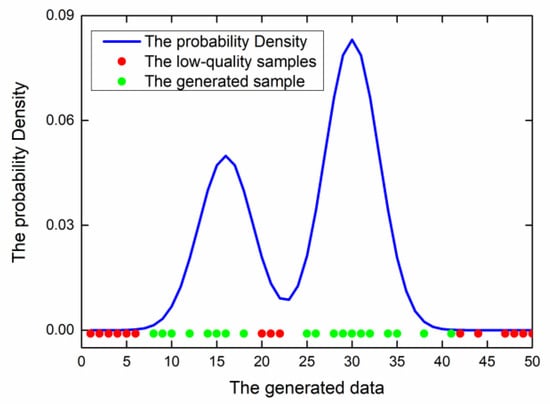
Figure 5.
The low-quality samples in actual situations.
The target of a GAN is to generate green samples instead of red samples. On the other hand, mode collapse restricts the diversity of the generated samples; that is, the generated samples are repetitive, similar, and lack modes, as shown in Figure 6.
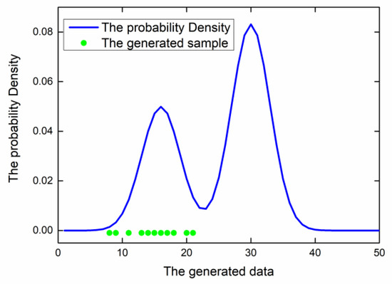
Figure 6.
The duplicate samples and missing modes.
Because there are many regional Nash equilibrium states in a GAN, the parameter optimization is not a convex majorization problem. Even if a GAN enters a certain Nash equilibrium state and the loss function appears to converge, mode collapse may still occur. Mode collapse is usually accompanied by such a phenomenon: when the discriminator updates the parameters near the training samples, the gradient value is so large. Therefore, the solution of mode collapse is that the discriminator is near the training sample to impose a gradient penalty term δ, which is given by
The proposed method attempts to construct a linear function near the training samples, because the linear function is a convex function and has a global optimal solution. The gradient penalty term is designed to improve GAN model and avoid mode collapse.
By way of the reciprocal adversarial learning between D and G, the capability of D and G is progressive. It has been proven that when Pg = Pdata, the distribution of the sample generated by G ideally matches the original fault-sample distribution. Moreover, the cross-entropy loss value converges to the Nash equilibrium when the output of D equals 0.5 [36]. Algorithm 1 shows the training algorithm of the GAN approach for generating new samples to augment the number of faulty samples.
| Algorithm 1. Training process of the generative adversarial network (GAN). Minibatch stochastic gradient descent (SGD) training for the GAN approach. The number of steps to apply to D was a hyper parameter (k). In the data augmentation experiments, k = 1 was used, which was the least expensive option. |
|
| end for |
| Any normal gradient-based learning regulation was used by the gradient-based updates, and the momentum was also used in the data augmentation experiments. |
As mentioned earlier, it is necessary to check the uncertainty of the generated samples. Therefore, a Gaussian-distribution cloud model was integrated into the GAN approach to evaluate this uncertainty. The mean and variance S2 of the generated samples are easily obtained. The entropy En of the generated samples is calculated as follows:
where Ex refers to the expectation of the generated samples and is given by . In the next step, the hyper entropy term (He) is the uncertainty index of En. It incarnates the dispersion degree of the cloud droplets that make up the cloud model. The He value is given by
In the cloud model, we suppose l is satisfied: , where . The degree of membership function for the fuzziness of the generated samples is written as follows:
The calculated membership function is fed back to the GAN approach and can reduce the uncertainty of the generated samples. The GAN approach is improved to generate samples by integrating into the Gaussian-distribution cloud model for data quality. The cloud model is demonstrated in Section 3. In Section 2.3, the samples generated by the GAN and the cloud model analysis provide high-quality training samples for the SDAE model.
2.3. Stacked Denoising Auto-Encoder
The SDAE consists of multiple denoising auto-encoders (DAE) through stacking [37]. The SDAE can provide extensive and vigorous fault-feature extraction from raw-input vibration data. The structure of the SDAE is composed of neural networks, as shown in Figure 7.
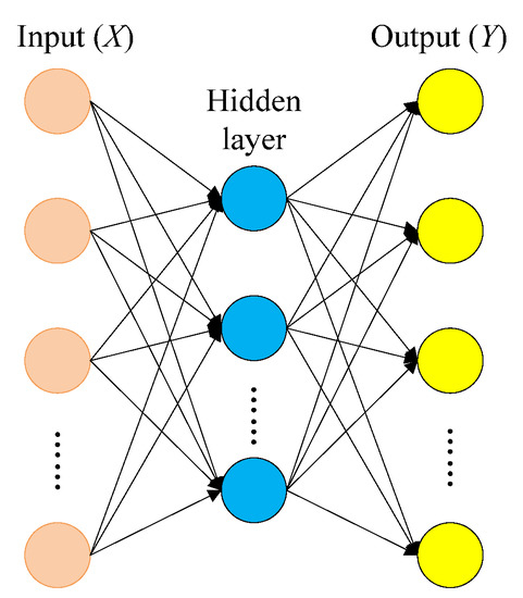
Figure 7.
Neural networks of the stacked denoising auto-encoder (SDAE).
The auto-encoder includes an encoding network and a decoding network. The encoding network maps the input vector X = {x1, …, xi} to the encoded vector, which is subsequently remapped to the output vector Y by the decoding network. The encoded vector is the characteristic representation of the input vector, whereas the output vector is the reconstruction representation of the input vector. The dimension of the output vector is equal to the input vector. The output of the encoding network is expressed as
where W = {w1, w2, …, wn} and B = {b1, b2, …, bn} are the weight matrix and the bias matrix, respectively, from the input layer to the hidden layer; and W and B constitute the parameter θ = {W, B}. Generally, the activation function S is a sigmoid function. The function of W and B is able to be summarized as the encoding of original data. SDAE decodes the output of the hidden layer using the following equation:
Constructing the SDAE model mainly determines the model parameters. The equation to solve the optimal parameters θ and θT is as follows:
To obtain the features of the input data, the loss function of SDAE must be reduced as much as possible. Like the traditional auto-encoder, the SGD algorithm is used to minimize the model error of SDAE. The loss function L(X, Z) is expressed by
The principle of SDAE is shown in Figure 8. As a typical deep learning method, SDAE has its own shortcomings. When the training vibration-fault samples are inadequate, the training on the SDAE model is also insufficient and the model cannot accurately obtain the parameter θ. This means that the SDAE-based fault diagnosis is inaccurate. However, as mentioned above, the GAN can generate many training samples after the data augmentation, and this can compensate for the shortcomings of the SDAE. A joint model combining GAN and SDAE—a GAN-SDAE system—is the best solution to improve the accuracy of the fault diagnosis.
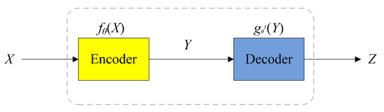
Figure 8.
Working principle of the SDAE.
2.4. Model Fusion and Evaluation
Model fusion merges multiple weak models into a strong model, which reduces the tendency of a single model to be overfitted. The fusion of multiple models can improve the normalization ability. It avoids the case wherein the single model is unstable with a low fault diagnosis ability. Multiple models can often improve the fault diagnosis ability and the robustness of the model significantly.
Waterfall model fusion uses a method of connecting multiple models in series. Each recommendation algorithm is regarded as a model. Waterfall model fusion connects models with different functions back and forth, as shown in Figure 9.
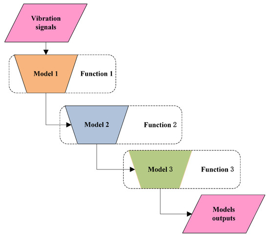
Figure 9.
Waterfall model fusion.
In the waterfall fusion, the target result achieved by the previous recommendation method can be used as the input of the latter method, progressively step by step. The function of the fusion model is gradually enhanced, and finally a result set with a low quantity and high quality is obtained. It is usually used to implement the recommended scenarios for different model functions. In designing a waterfall model-fusion method, the model functions are usually sequenced and gradually transitioned to achieve the final goal. In the face of a large number of candidate recommendation objects, but few valuable recommendation results, high accuracy requirements and limited computing time, it is often suitable.
The small fault-sample regeneration model (GAN) and SDAE model are a series of two single models, adopting the waterfall-type in model fusion. The GAN-SDAE structure is shown in Figure 10. The GAN-SDAE system based on waterfall model fusion strengthens the model’s fault tolerance rate and improves the accuracy of the integrated learning.
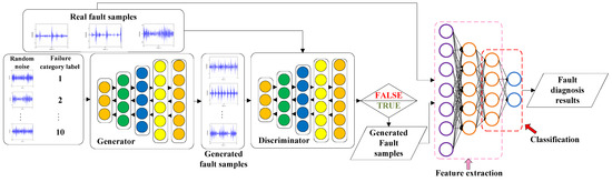
Figure 10.
Waterfall model fusion for the GAN-SDAE system.
For the GAN-SDAE system, the number of neurons is more significant than the layer thickness in the case of small fault samples [38]. The number of layers for both GAN and SDAE is three or four each. To construct an optimal GAN-SDAE system structure, a reconstruction error in the deep networks is proposed [39]. The reconstruction errors of each sample from the GAN-SDAE were obtained in a training process for a fault diagnostic task. Because the real fault diagnosis result (C) for each sample is known, the diagnostic error can be calculated. The output result from the GAN-SDAE system is Z, and the reconstruction error Ɛ in the training process is given by Ɛ = |C − Z|.
Different reconstruction errors for different network structures were calculated. The network structure having the least reconstruction error was finally selected as the optimal structure (the various network structures of GAN-SDAE and corresponding reconstruction errors are analyzed in Section 3). Combining the analyses in Section 2.2 and Section 2.3 provides an overall flow chart of using GAN-SDAE for machine fault diagnosis; this is shown in Figure 11.

Figure 11.
Flow chart of the GAN-SDAE system for fault diagnosis.
Evaluation indicators are regarded as developers showing the results to users and making standardized comparisons. Moreover, evaluation indicators can illustrate the appropriate expression of needs and scientific information. Over the years, due to the practice of fault diagnosis methods in various disciplines, various index sets have been established in the field of fault diagnosis to evaluate model performance [40]. The metric sets are mainly designed to verify the performance of the GAN-SDAE system’s applications. Therefore, evaluation indicators are particularly important in the model development phase, which can be used to improve the fault diagnosis program.
The error is basically expressed as a deviation from the desired target. Most of the accuracy-based metrics are derived directly or indirectly from the error term. The error is expressed as
where is the estimated value and yi is the expected output value. According to the error definition, the absolute error (AE) is given by
Considering that there are multiple instances, the mean absolute error (MAE) calculates the average of the absolute error term. The quantity is used to measure how close the estimate is to the final result. MAE is expressed by
The mean square error (MSE) is a hazard function that calculates the average of the squared error. MSE can be estimated in the following way:
The mean absolute deviation from the sample median (MAD), which is an estimate of the resistance to changes in the result errors, is given by
Root mean square error (RMSE) is a measure of the deviation between the observed value and the true value. It is often used as a standard for measuring the output results of machine learning models. RMSE is expressed by
The performance evaluation indexes are completely used to provide accurate verification of the GAN-SDAE system, especially in vibration signals, to accurately evaluate the fault diagnosis performance.
2.5. Analysis of Uncertainty in a GAN-SDAE
In Section 2.2, a Gaussian-distributed cloud model was built to analyze the uncertainty of the samples generated by the GAN approach. Similarly, it was important to check the uncertainty of the GAN-SDAE system. This system contains a neural network structure, whose calculation method is essentially a black box; hence, the system has inherent instability. The reliability of a GAN-SDAE for machine fault diagnosis can be ensured by analyzing the uncertainty of the system [41]. As previously demonstrated [42], the system uncertainty can be analyzed through repetitive experiments. For the diagnostic result Z, n independent observations are repeatedly performed under reproducible conditions. Subsequently, the standard deviation S(Zi) of the fault diagnoses yielded by GAN-SDAE can be calculated. The term represents the standard uncertainty outcome for the GAN-SDAE system, scilicet, the A standard uncertainty, uA. The standard deviation is given by
Using non-statistical methods to evaluate the standard uncertainty of the proposed system yields B standard uncertainty (uB). In line with engineering experience and information related to the system, we analyzed the interval in which the fault diagnosis results were within [ − a, + a]. The a denotes the half-width of the confidence interval. With confidence level p, the inclusion factor k is calculated. The uB can be expressed by uB = a/k. The synthetic standard uncertainty (uC), which characterizes the degree of the dispersion from GAN-SDAE system experiments, is written as
where the sensitivity coefficients of uA and uB are severally k1 and k2.
3. Experimental Validation
3.1. Vibration Data Description
The vibration data of the ball bearings were collected from a motor-driven test rig [43]. The test instruments mostly are composed of an induction motor (Reliance Electric 2HP IQPreAlert), a dynamometer, a torque sensor, an accelerometer, and other components.
The ball bearings have four conditions and the fault diameters with their labels are in Table 1. In the fault diagnosis experiment, ten distinct fault types, under loads of 1, 2, or 3 hp, were divided into datasets A, B, C, and D. Each type of each dataset contained 600 training samples and 200 test samples. Dataset D contained all three loads. Four datasets were tested by the fault diagnosis model under different load conditions.

Table 1.
Datasets for the ball-bearing faults.
Each sample contained 2048 data points; hence, it was appropriate to implement a fast Fourier transformation (FFT) on the samples. All the test and training data in datasets A, B, C, and D were normalized to render the vibration data comparable with each other. Due to the limited amount of original vibration data with bearing faults, GAN data augmentation was applied to the training data.
3.2. Parameters of the GAN-SDAE
The training samples were inputted into the training network of the GAN-SDAE system. When the system was trained to a stable condition, the test samples were inputted into the GAN-SDAE system to test the system. The system output was the fault type; the fault-diagnosis accuracy was also calculated. As mentioned earlier, the accuracy of fault diagnosis depends on the structure of the GAN-SDAE network, containing many layers and neurons. The reconstruction errors were analyzed to determine the optimal network structure. The calculated reconstruction errors are shown in Table 2. In addition, we found a new phenomenon: training the same network structure of G and D performed better than using different network structures. The same-network training results ensured the quality of the generated samples and a high accuracy in the fault diagnosis. On the basis of the reconstruction error, the network structures of G and D have three layers, which respectively have four, four, and one neuron(s). The structure of the SDAE network is four layers, which respectively have three, three, two, and one neuron(s).
Table 2.
Reconstruction error of the different network structures.
3.3. Data Augmentation
Like other deep learning methods, there are many parameters in the SDAE model. A vast number of training samples are necessary for training the SDAE so as to avoid overfitting and improve the generalization. In addition, training samples are balanced or imbalanced, which can cause differences in the diagnostic results [44,45]. The accuracy of fault diagnosis is usually affected by the imbalance of datasets. However, datasets A, B, C, and D were all balanced.
According to the previous introduction (Section 2.2), we needed to check the Nash balance point to verify whether G and D were in the trained convergence state. The result for all data reached the Nash equilibrium point. The calculation result, based on the Label 2 type of Dataset A, is shown in Figure 12 as an example. This method was applicable to other datasets.

Figure 12.
Probability value of the D output.
Figure 13 shows the original vibration sample of the Label 2 type of Dataset A and its corresponding generated samples. Other fault-type generated samples were similar. The generated samples differed from the original sample and the original training samples were extended by the generated ones.
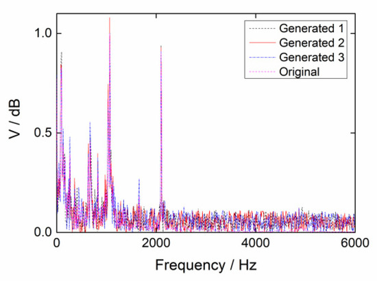
Figure 13.
Original and generated samples.
The uncertainty analysis for the generated samples of the Label 2 type of Dataset A is shown in Figure 14. The analysis of other generated fault samples was similar. We concluded that the generated samples conformed to the 3δ principle and that the membership function obeyed a Gaussian distribution using the cloud model. Therefore, the generated samples were feasible for SDAE training.
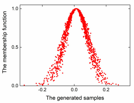
Figure 14.
The membership function of the generated samples.
Enough training samples were obtained to investigate how many training samples were sufficient and how well the SDAE performed. Different numbers of training samples as generated by the GAN approach were fed into the SDAE to test its performance. These amounts were selected as 700, 750, 800, 850, 900, 950, 1000, 1050, and 1100 samples in the experiment. The results with varying amounts of training samples are shown in Figure 15.
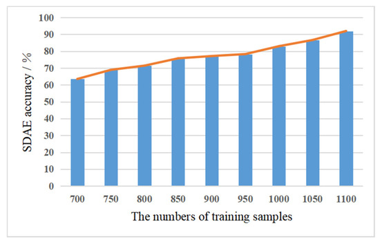
Figure 15.
Fault diagnosis results with varying amounts of training samples.
It is evident that the performance of the SDAE for fault diagnosis improved as the volume of the training samples increased, with an increase of 30% in accuracy from 700 samples to 1100 samples. With 1000 training samples, the accuracy of the fault diagnosis was above 80%. When the samples were increased to 1100, the accuracy of the SDAE peaked at 92.01%. Considering the cost of the calculation, we made a compromise by expanding the sample size to 1100 without increasing the amount of data. The random-noise data were inputted into the GAN for data augmentation and were converted into vibration fault data, based on adversarial learning. This approach makes up for the shortcomings of other methods, such as oversampling. Because GAN data augmentation expands the count of the training samples, the training performance of the SDAE is intensified and the generalization of the SDAE is further increased.
3.4. Performance of the GAN-SDAE System
Deep learning can adaptively mine vibration-fault features from the signal spectra. To examine the feature-mining capability of the GAN-SDAE, we used t-SNE to extract the features from the output of the last layer of the GAN-SDAE. The details of the t-SNE algorithm have been documented [46]. Visual analysis of the categories for Label 1 to Label 10 based on the t-SNE is shown in Figure 16. It is evident that the t-SNE was able to group the faults according to their types and that this method accurately distinguished ten types.
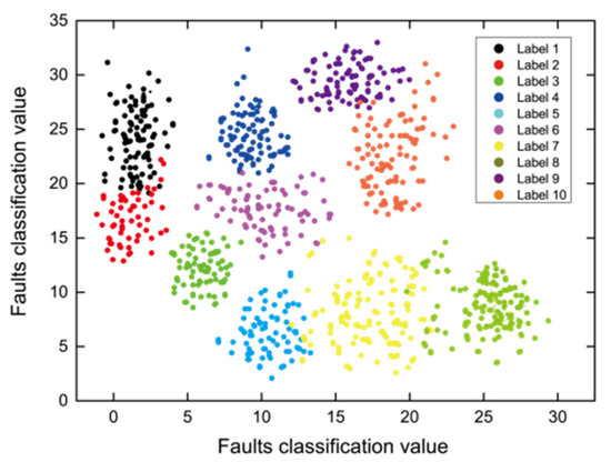
Figure 16.
Feature visualization through t-SNE.
The performance of the GAN-SDAE was tested using four datasets in different load domains. The diagnostic results from the proposed GAN-SDAE were compared with those from SDAE. They were also compared with the results from classic machine learning algorithms, namely support vector machine (SVM), back propagation networks (BPN), and DAE. The comparisons are shown in Figure 17.

Figure 17.
Accuracy of different fault diagnosis methods.
It is evident that the accuracy of GAN-SDAE for all four loads was above 90% and was higher than the accuracy of the other four methods. The accuracy from SDAE was above 80%, which was higher than other traditional machine learning methods. The SVM performed worst in the comparison, with an average accuracy below 75%. In summary, with the support of GAN, the capability of the SDAE was markedly increased.
3.5. Baselines and Evaluation
The baselines for bearing fault diagnosis were set as per References [47,48,49]. The effect of vibration signal fault diagnosis is shown in Figure 18. Obviously, the GAN-SDAE system proposed in this paper has a higher average accuracy rate than the baselines in the references, so it improved the accuracy of the fault diagnosis.
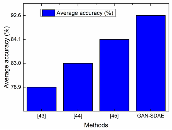
Figure 18.
The results of comparing GAN-SDAE with the methods.
The MAE, MSE, MAD, RMSE for the GAN-SDAE system are shown in Table 3. The proposed method evaluation is satisfactory. By using improved data enhancement methods, the SDAE model can complete learning and training on demand, while significantly improving the performance.
Table 3.
GAN-SDAE system evaluation indexes.
As mentioned previously, all current deep learning algorithms inherently face the problem of system uncertainty; furthermore, non-convergence may happen during network training. Therefore, besides the accuracy requirement for fault diagnosis, the stability of the system must be checked. The uncertainty analysis was performed to ensure the stability of the GAN-SDAE. The GAN-SDAE system was used to conduct repetitive experiments in various load domains. The synthetic standard uncertainty uC for the four datasets (four loads) is illustrated in Figure 19. Overall, the value of uC decreased as the number of repetitive experiments increased. When the number of repetitive experiments was above 40, uC reached a stable condition at a 0.2 float.
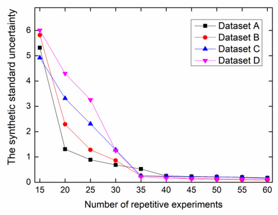
Figure 19.
The synthetic standard uncertainty, uC.
3.6. Versatility of GAN-SDAE System
The usefulness of the GAN-SDAE system was confirmed by the classic bearing fault diagnosis. However, in the actual industry, gear fault diagnosis is also common. To verify the applicability of GAN-SDAE, we applied this system to gear fault diagnosis. The gear fault signals were obtained by the drive-train dynamic simulator (DDS). The different types of faults in the gears are shown in Table 4 [50].
Table 4.
Description of gear fault types.
The process of data augmentation for the gears was similar to the bearing experiment. The number of samples in the training set increased from 900 to 1200, which achieved the purpose of expanding the training samples. Visual analysis of categories Label 1 to Label 5 based on t-SNE is shown in Figure 20. It is evident that the t-SNE for the GAN-SDAE grouped the same gear fault types together and accurately distinguished five gear types. The cluster analysis for the gears had the same effect as in the bearing experiment and these results confirmed that the gear-fault features extracted by the GAN-SDAE were separable.

Figure 20.
Feature visualization through t-SNE.
A comparison of gear fault diagnosis was conducted using the same comparison method as in Experiment A, including SVM, BPN, DAE, SDAE, and GAN-SDAE. The experimental results of the different methods are shown in Figure 21.

Figure 21.
The results of the gear fault diagnosis.
The results indicate that both SVM and BPN were less than 80% accurate. The accuracy of the DAE fault diagnosis was 80.23%, and the effect is common. The accuracy of the SDAE was 86.93%, and data augmentation by GAN increased this result to 90.35% for the proposed system. The uC of the GAN-SDAE for gears is shown in Figure 22. With above 40 repetitive experiments, uC was below 0.6. This result reflects the stability of the GAN-SDAE system for gear fault diagnosis.
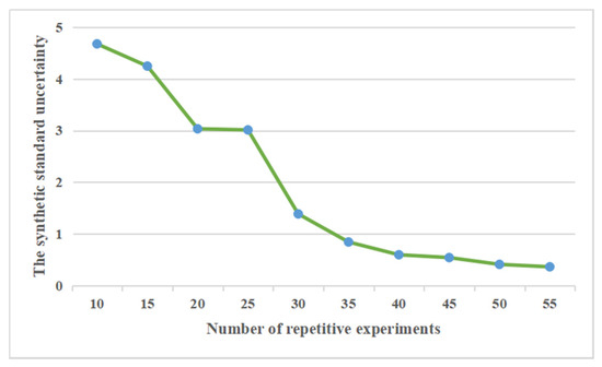
Figure 22.
The synthetic standard uncertainty.
4. Conclusions
A novel fault diagnosis method is proposed, based on a GAN-SDAE system. This proposed system combines the advantages of GAN, which is to learn an original sample distribution, and SDAE, which is to accurately diagnose faults. We drew conclusions from the experimental results for two cases of bearings and gears:
- (1)
- The optimal network structures of the bearing and gear fault diagnostic systems are determined by the reconstruction errors. We established two GAN-SDAE systems for bearings and gears, respectively. It is feasible to apply a GAN-SDAE to fault diagnosis.
- (2)
- As a result of the adversarial learning process, the generator and the discriminator of the GAN approach are trained in turn. We improved the GAN approach using a cloud model analysis, which improved the data augmentation. The data augmentation in turn improved the classification ability of the GAN-SDAE system.
- (3)
- The system uncertainty of the GAN-SDAE was analyzed by repetitive experiments. The synthetic standard uncertainty uC remained at a 0.2 float for bearing fault diagnosis and below 0.6 for the gear fault diagnosis. These results reflect the stability of the GAN-SDAE system.
- (4)
- The GAN-SDAE system was compared with other fault diagnosis models (SVM, BPN, DAE, and SDAE). The proposed system is obviously advanced.
- (5)
- The GAN-SDAE was showed an accuracy higher than 90% for both bearing and gear faults. This result reflects the adaptability of the proposed method.
Author Contributions
Conceptualization, Q.F. and H.W.; methodology, Q.F.; software, Q.F.; validation, Q.F.; formal analysis, Q.F.; investigation, Q.F.; resources, H.W.; data curation, H.W.; writing: original draft preparation, Q.F.; writing: review and editing, Q.F.; visualization, Q.F.; supervision, Q.F.; project administration, H.W.; funding acquisition, H.W. All authors have read and agreed to the published version of the manuscript.
Funding
This research was funded by the Natural Science Foundation of China, grant number U1833110.
Conflicts of Interest
The authors declare no conflict of interest.
References
- Thatoi, D.N.; Das, H.C.; Parhi, D.R. Review of Techniques for Fault Diagnosis in Damaged Structure and Engineering System. Adv. Mech. Eng. 2012, 4, 327569. [Google Scholar] [CrossRef]
- Agrawal, V.; Panigrahi, B.; Subbarao, P. Review of control and fault diagnosis methods applied to coal mills. J. Process. Control. 2015, 32, 138–153. [Google Scholar] [CrossRef]
- Choudhary, A.; Goyal, D.; Shimi, S.L.; Akula, A. Condition Monitoring and Fault Diagnosis of Induction Motors: A Review. Arch. Comput. Methods Eng. 2018, 26, 1221–1238. [Google Scholar] [CrossRef]
- Razavi-Far, R.; Hallaji, E.; Farajzadeh-Zanjani, M.; Saif, M.; Kia, S.H.; Henao, H.; Capolino, G.-A. Information Fusion and Semi-Supervised Deep Learning Scheme for Diagnosing Gear Faults in Induction Machine Systems. IEEE Trans. Ind. Electron. 2018, 66, 6331–6342. [Google Scholar] [CrossRef]
- Zhang, Z.; Li, S.; Wang, J.; Xin, Y.; An, Z. General normalized sparse filtering: A novel unsupervised learning method for rotating machinery fault diagnosis. Mech. Syst. Signal Process. 2019, 124, 596–612. [Google Scholar] [CrossRef]
- Khare, N.; Devan, P.; Chowdhary, C.L.; Bhattacharya, S.; Singh, G.; Singh, S.; Yoon, B. SMO-DNN: Spider Monkey Optimization and Deep Neural Network Hybrid Classifier Model for Intrusion Detection. Electron 2020, 9, 692. [Google Scholar] [CrossRef]
- Liang, J.; Zhang, Y.; Zhong, J.-H.; Yang, H. A novel multi-segment feature fusion based fault classification approach for rotating machinery. Mech. Syst. Signal Process. 2019, 122, 19–41. [Google Scholar] [CrossRef]
- Wang, J.; Li, S.; Xin, Y.; An, Z. Gear Fault Intelligent Diagnosis Based on Frequency-Domain Feature Extraction. J. Vib. Eng. Technol. 2019, 7, 159–166. [Google Scholar] [CrossRef]
- Arik, S. A New Lyapunov Analysis of Robust Stability of Neural Networks with Discrete Time Delays. In Proceedings of the 21st EANN (Engineering Applications of Neural Networks) 2020 Conference, Porto Carras Grand Resort, Halkidiki, Greece, 5–7 June 2020; Springer Science and Business Media: Berlin, Germany, 2020; pp. 523–534. [Google Scholar]
- Lu, C.; Wang, Z.-Y.; Qin, W.-L.; Ma, J. Fault diagnosis of rotary machinery components using a stacked denoising autoencoder-based health state identification. Signal Process. 2017, 130, 377–388. [Google Scholar] [CrossRef]
- Guo, X.; Shen, C.; Chen, L. Deep Fault Recognizer: An Integrated Model to Denoise and Extract Features for Fault Diagnosis in Rotating Machinery. Appl. Sci. 2016, 7, 41. [Google Scholar] [CrossRef]
- Xia, M.; Li, T.; Liu, L.; Xu, L.; De Silva, C.W. Intelligent fault diagnosis approach with unsupervised feature learning by stacked denoising autoencoder. IET Sci. Meas. Technol. 2017, 11, 687–695. [Google Scholar] [CrossRef]
- Sengupta, S.; Basak, S.; Saikia, P.; Paul, S.; Tsalavoutis, V.; Atiah, F.; Ravi, V.; Peters, A. A review of deep learning with special emphasis on architectures, applications and recent trends. Knowl.-Based Syst. 2020, 194, 105596. [Google Scholar] [CrossRef]
- Sulikowski, P.; Zdziebko, T. Deep Learning-Enhanced Framework for Performance Evaluation of a Recommending Interface with Varied Recommendation Position and Intensity Based on Eye-Tracking Equipment Data Processing. Electronics 2020, 9, 266. [Google Scholar] [CrossRef]
- Rosenshield, G.; Prokhorov, A.M. The Great Soviet Encyclopedia. Slav. East Eur. J. 1975, 19, 366. [Google Scholar] [CrossRef]
- Dai, Z.; Wang, Z.; Jiao, Y. Bayes Monte-Carlo Assessment Method of Protection Systems Reliability Based on Small Failure Sample Data. IEEE Trans. Power Deliv. 2014, 29, 1841–1848. [Google Scholar] [CrossRef]
- Roh, Y.; Heo, G.; Whang, S.E. A Survey on Data Collection for Machine Learning: A Big Data—AI Integration Perspective. IEEE Trans. Knowl. Data Eng. 2019, 1. [Google Scholar] [CrossRef]
- Goodfellow, I.; Pouget-Abadie, J.; Mirza, M.; Xu, B.; Warde-Farley, D.; Ozair, S.; Courville, A.; Bengio, Y. Generative Adversarial Networks. arXiv 2014, arXiv:1406.2661. [Google Scholar]
- Wang, Y.; Yu, B.; Wang, L.; Zu, C.; Lalush, D.S.; Lin, W.; Wu, X.; Zhou, J.; Shen, D.; Zhou, L. 3D conditional generative adversarial networks for high-quality PET image estimation at low dose. NeuroImage 2018, 174, 550–562. [Google Scholar] [CrossRef]
- Ma, J.; Yu, W.; Liang, P.; Li, C.; Jiang, J. FusionGAN: A generative adversarial network for infrared and visible image fusion. Inf. Fusion 2019, 48, 11–26. [Google Scholar] [CrossRef]
- Zhang, C.; Wu, L.; Wang, Y.; Long, J. Crossing generative adversarial networks for cross-view person re-identification. Neurocomputing 2019, 340, 259–269. [Google Scholar] [CrossRef]
- Liu, S.; Yu, M.; Li, M.; Xu, Q. The research of virtual face based on Deep Convolutional Generative Adversarial Networks using TensorFlow. Phys. A: Stat. Mech. its Appl. 2019, 521, 667–680. [Google Scholar] [CrossRef]
- Ghorban, F.; Milani, N.; Schugk, D.; Roese-Koerner, L.; Su, Y.; Muller, D.; Kummert, A. Conditional multichannel generative adversarial networks with an application to traffic signs representation learning. Prog. Artif. Intell. 2018, 8, 73–82. [Google Scholar] [CrossRef]
- Li, X.; Zhang, W.; Ding, Q. Cross-Domain Fault Diagnosis of Rolling Element Bearings Using Deep Generative Neural Networks. IEEE Trans. Ind. Electron. 2019, 66, 5525–5534. [Google Scholar] [CrossRef]
- Mao, W.; Liu, Y.; Ding, L.; Li, Y. Imbalanced Fault Diagnosis of Rolling Bearing Based on Generative Adversarial Network: A Comparative Study. IEEE Access 2019, 7, 9515–9530. [Google Scholar] [CrossRef]
- Wen, W.; Bai, Y.; Cheng, W. Generative Adversarial Learning Enhanced Fault Diagnosis for Planetary Gearbox under Varying Working Conditions. Sensors 2020, 20, 1685. [Google Scholar] [CrossRef]
- Liu, K.; Qiu, G.; Tang, W.; Zhou, F. Spectral Regularization for Combating Mode Collapse in GANs. In Proceedings of the 2019 IEEE/CVF International Conference on Computer Vision (ICCV), Seoul, Korea, 27 October–3 November 2019; Institute of Electrical and Electronics Engineers (IEEE): Piscataway, NJ, USA, 2019; pp. 6381–6389. [Google Scholar]
- Lei, Y. A Deep Learning-based Method for Machinery Health Monitoring with Big Data. Chin. J. Mech. Eng. 2015, 51, 49–56. [Google Scholar] [CrossRef]
- Yang, J.; Xie, G.; Yang, Y. An improved ensemble fusion autoencoder model for fault diagnosis from imbalanced and incomplete data. Control. Eng. Pr. 2020, 98, 104358. [Google Scholar] [CrossRef]
- Wang, T.; Dong, J.; Xie, T.; Diallo, D.; Benbouzid, M. A Self-Learning Fault Diagnosis Strategy Based on Multi-Model Fusion. Information 2019, 10, 116. [Google Scholar] [CrossRef]
- Komatsu, A. Vibration transducer. J. Acoust. Soc. Am. 2003, 114, 1214. [Google Scholar]
- Drahm, W.; Rieder, A. Transducer of the vibration type, such as an electromechanical transducer of the coriollis type. J. Acoust. Soc. Am. 2005, 117, 1698. [Google Scholar] [CrossRef]
- Lei, Y. Individual intelligent method-based fault diagnosis. In Intelligent Fault Diagnosis and Remaining Useful Life Prediction of Rotating Machinery; Elsevier: Amsterdam, The Netherlands, 2017; pp. 67–174. [Google Scholar]
- Wang, K.F.; Gou, C.; Duan, Y.J.; Lin, Y.-L.; Zheng, X.H.; Wang, F.Y. Generative Adversarial Networks: The State of the Art and Beyond. Acta Autom. Sinica 2017, 43, 321–332. [Google Scholar]
- Zhang, P.; Qiao, H.; Zhang, B. An improved local tangent space alignment method for manifold learning. Pattern Recognit. Lett. 2011, 32, 181–189. [Google Scholar] [CrossRef]
- Ratliff, L.J.; Burden, S.A.; Sastry, S.S. Characterization and computation of local Nash equilibria in continuous games. In Proceedings of the 51st Annual Allerton Conference on Communication, Control, and Computing, Monticello, IL, USA, 2–4 October 2013; pp. 917–924. [Google Scholar]
- Tong, C.; Li, J.; Lang, C.; Kong, F.; Niu, J.; Rodrigues, J.J.P.C. An efficient deep model for day-ahead electricity load forecasting with stacked denoising auto-encoders. J. Parallel Distrib. Comput. 2018, 117, 267–273. [Google Scholar] [CrossRef]
- Coates, A.; Lee, H.; Ng, A. An analysis of single-layer networks in unsupervised feature learning. J. Mach. Learn. Res. 2011, 15, 215–223. [Google Scholar]
- Jiang, J.; Zhang, J.; Zhang, L.; Ran, X.; Jiang, J.; Wu, Y. DBN Structure Design Algorithm for Different Datasets Based on Information Entropy and Reconstruction Error. Entropy 2018, 20, 927. [Google Scholar] [CrossRef]
- Goebel, K.; Saha, B.; Saxena, A.; Celaya, J.; Christophersen, J. Prognostics in Battery Health Management. IEEE Instrum. Meas. Mag. 2008, 11, 33–40. [Google Scholar] [CrossRef]
- Samli, R.; Yucel, E. Global robust stability analysis of uncertain neural networks with time varying delays. Neurocomputing 2015, 167, 371–377. [Google Scholar] [CrossRef]
- Fernández, M.S.-B.; Calderón, J.M.A.; Díez, P.M.B. Implementation in MATLAB of the adaptive Monte Carlo method for the evaluation of measurement uncertainties. Accredit. Qual. Assur. 2008, 14, 95–106. [Google Scholar] [CrossRef]
- Lou, X.; Loparo, K.A. Bearing fault diagnosis based on wavelet transform and fuzzy inference. Mech. Syst. Signal Process. 2004, 18, 1077–1095. [Google Scholar] [CrossRef]
- Villa, L.F.; Reñones, A.; Perán, J.R.; Miguel, L.J. Angular resampling for vibration analysis in wind turbines under non-linear speed fluctuation. Mech. Syst. Signal Process. 2011, 25, 2157–2168. [Google Scholar] [CrossRef]
- Santos, P.; Maudes, J.M.; Bustillo, A. Identifying maximum imbalance in datasets for fault diagnosis of gearboxes. J. Intell. Manuf. 2015, 29, 333–351. [Google Scholar] [CrossRef]
- Dhalmahapatra, K.; Shingade, R.; Mahajan, H.; Verma, A.; Maiti, J. Decision support system for safety improvement: An approach using multiple correspondence analysis, t-SNE algorithm and K-means clustering. Comput. Ind. Eng. 2019, 128, 277–289. [Google Scholar] [CrossRef]
- Melin, P.; Amezcua, J.; Valdez, F.; Castillo, O. A new neural network model based on the LVQ algorithm for multi-class classification of arrhythmias. Inf. Sci. 2014, 279, 483–497. [Google Scholar] [CrossRef]
- Karabadji, N.E.I.; Seridi, H.; Khelf, I.; Azizi, N.; Boulkroune, R. Improved decision tree construction based on attribute selection and data sampling for fault diagnosis in rotating machines. Eng. Appl. Artif. Intell. 2014, 35, 71–83. [Google Scholar] [CrossRef]
- Sakthivel, N.; Sugumaran, V.; Babudevasenapati, S. Vibration based fault diagnosis of monoblock centrifugal pump using decision tree. Expert Syst. Appl. 2010, 37, 4040–4049. [Google Scholar] [CrossRef]
- Shao, S.; McAleer, S.; Yan, R.; Baldi, P. Highly Accurate Machine Fault Diagnosis Using Deep Transfer Learning. IEEE Trans. Ind. Inform. 2019, 15, 2446–2455. [Google Scholar] [CrossRef]
© 2020 by the authors. Licensee MDPI, Basel, Switzerland. This article is an open access article distributed under the terms and conditions of the Creative Commons Attribution (CC BY) license (http://creativecommons.org/licenses/by/4.0/).