Figure 1.
Graph of the hidden Markov model.
Figure 1.
Graph of the hidden Markov model.
Figure 2.
Initial log-diffusivity field with observation locations , monitoring locations ×, and heat source ∆.
Figure 2.
Initial log-diffusivity field with observation locations , monitoring locations ×, and heat source ∆.
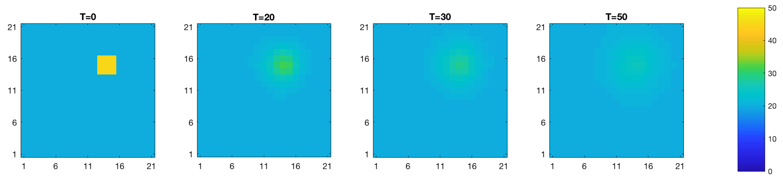
Figure 3.
True temperature (C) field evolution over time.
Figure 3.
True temperature (C) field evolution over time.
Figure 4.
Data collected over time () and true temperature evolution (line) at the data collection points.
Figure 4.
Data collected over time () and true temperature evolution (line) at the data collection points.
Figure 5.
Realizations from the initial selection-Gaussian distribution of the log diffusivity at time (upper panels) and associated spatial histogram (lower panels). Lower panels: the horizontal axes represent the log-diffusivity, the vertical axes represent the relative prevalence of each log-diffusivity value for the realization in the panel right above.
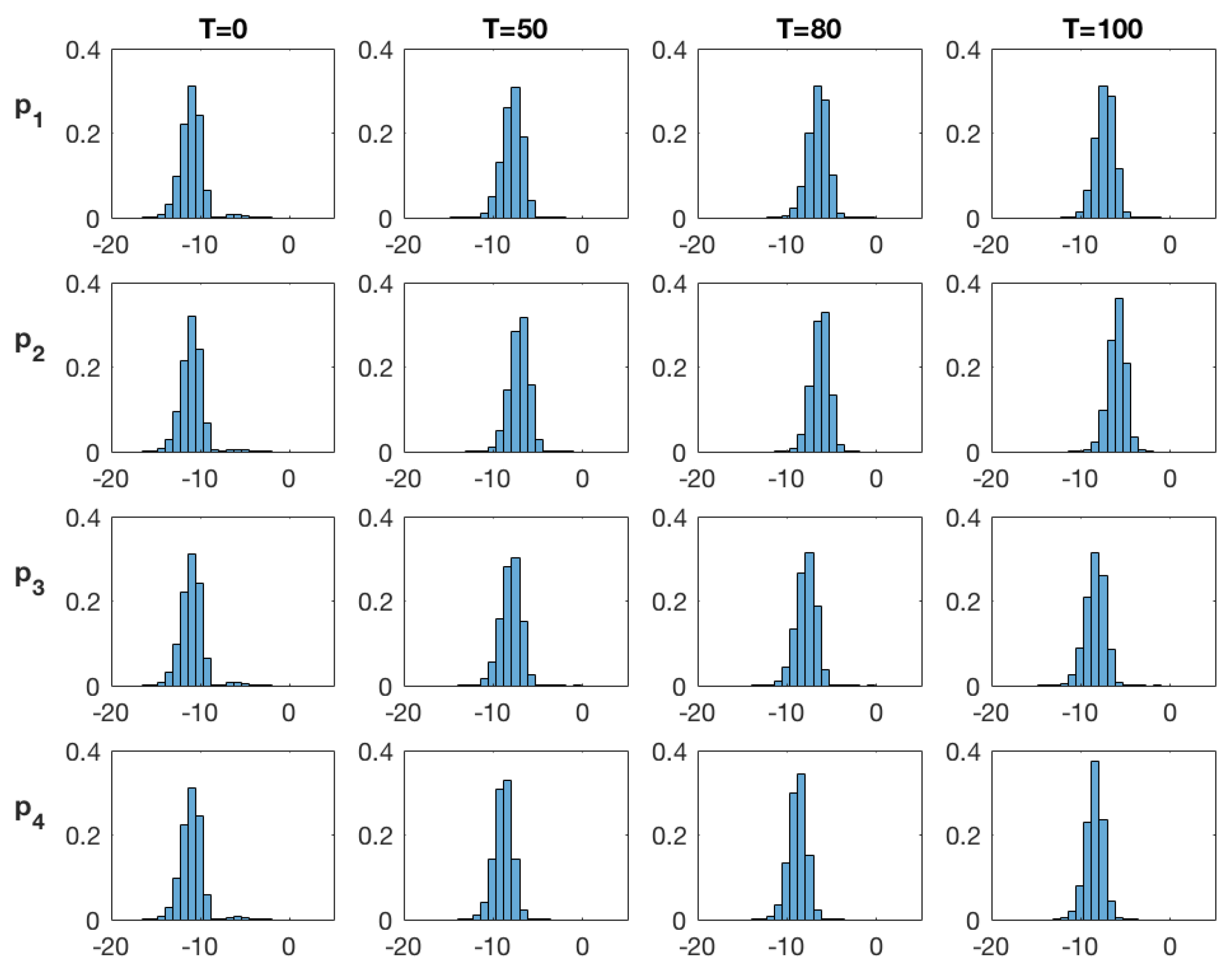
Figure 6.
SEnKF approach: Marginal posterior distribution of the log diffusivity at time at the monitoring locations () denoted ().
Figure 6.
SEnKF approach: Marginal posterior distribution of the log diffusivity at time at the monitoring locations () denoted ().
Figure 7.
EnKF approach: Marginal posterior distribution of the log diffusivity at time at the monitoring locations () denoted ().
Figure 7.
EnKF approach: Marginal posterior distribution of the log diffusivity at time at the monitoring locations () denoted ().
Figure 8.
MMAP predictions of the log diffusivity field at time (upper panels—SEnKF approach, lower panels—EnKF approach).
Figure 8.
MMAP predictions of the log diffusivity field at time (upper panels—SEnKF approach, lower panels—EnKF approach).
Figure 9.
MMAP predictions of the log diffusivity field with HDI in cross section B-B’ at time with SEnKF (left) and with EnKF (right).
Figure 9.
MMAP predictions of the log diffusivity field with HDI in cross section B-B’ at time with SEnKF (left) and with EnKF (right).
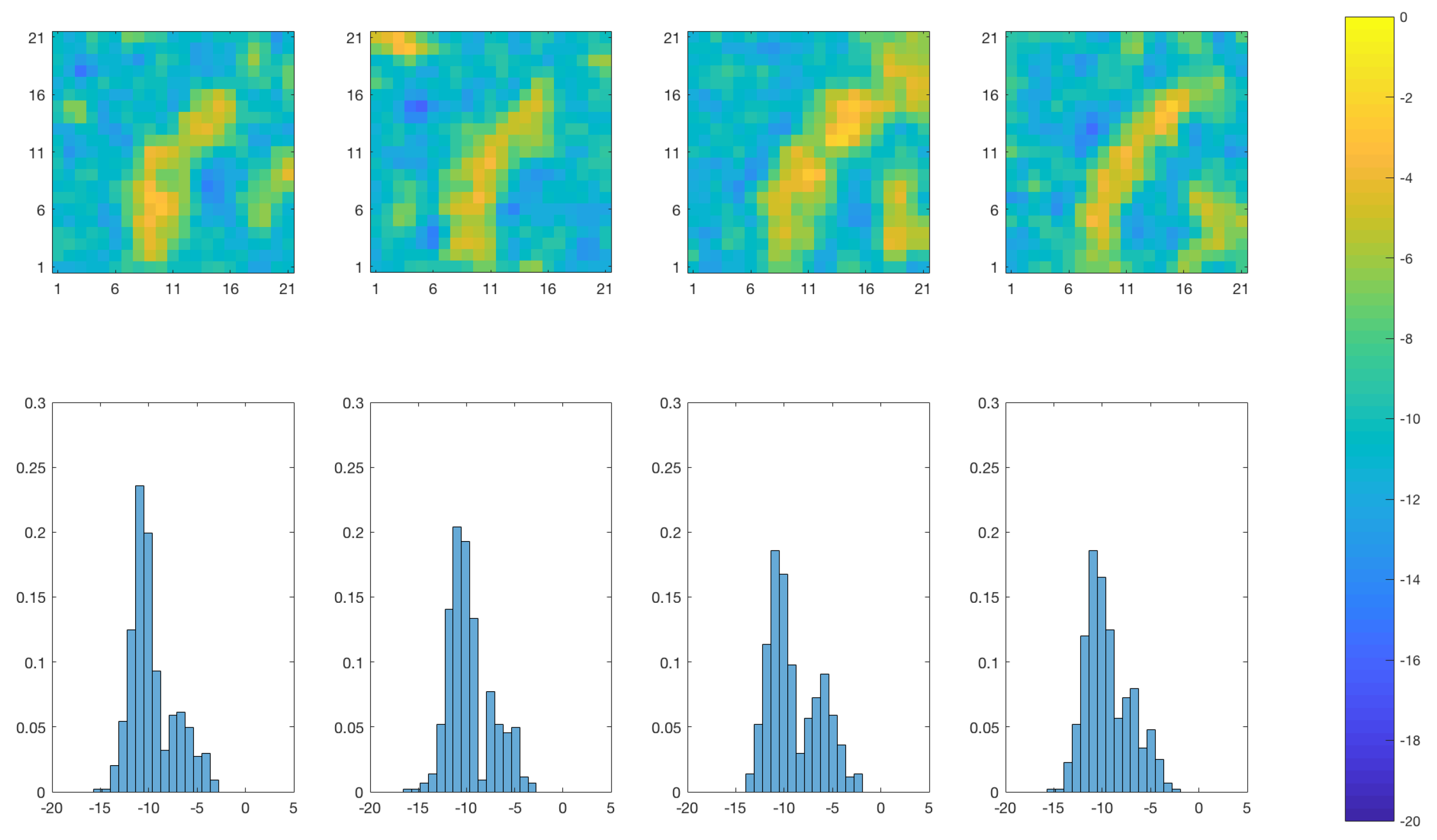
Figure 10.
SEnKF approach: Realizations of the posterior distribution of the log diffusivity at time (upper panels) and associated spatial histogram (lower panels). Lower panels: the horizontal axes represent the log-diffusivity, the vertical axes represent the relative prevalence of each log-diffusivity value for the realization in the panel right above.
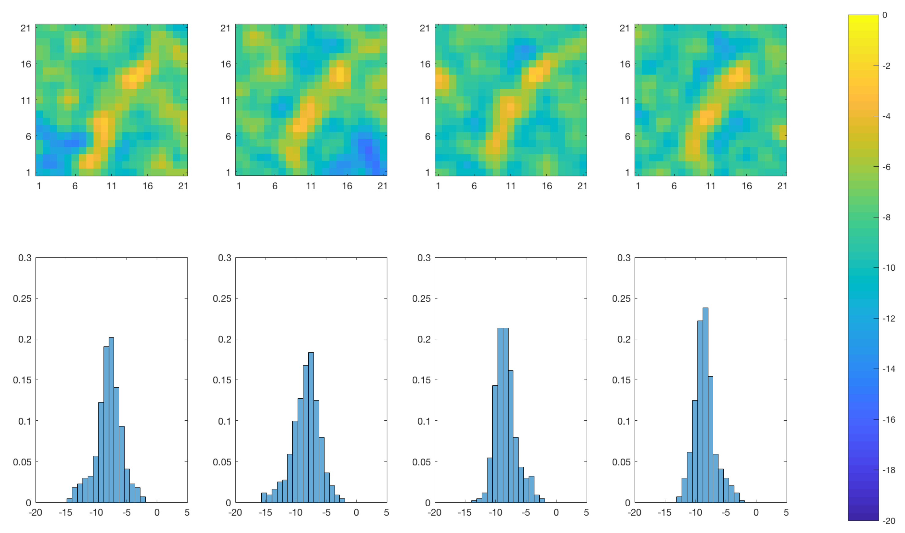
Figure 11.
EnKF approach: Realizations of the posterior distribution of the log diffusivity at time (upper panels) and associated spatial histogram (lower panels). Lower panels: the horizontal axes represent the log-diffusivity, the vertical axes represent the relative prevalence of each log-diffusivity value for the realization in the panel right above.
Figure 12.
Initial temperature (C) field (left) with data collection points and monitoring locations × and reference log-diffusivity field (right).
Figure 12.
Initial temperature (C) field (left) with data collection points and monitoring locations × and reference log-diffusivity field (right).
Figure 13.
True temperature (C) field evolution over time.
Figure 13.
True temperature (C) field evolution over time.
Figure 14.
Data collected over time (points) and true temperature (C) evolution at the data collection points (line).
Figure 14.
Data collected over time (points) and true temperature (C) evolution at the data collection points (line).
Figure 15.
Realizations from the selection-Gaussian initial distribution of the initial temperature field at time (upper panels) and associated spatial histogram (lower panels). Upper panels: the colorbar gives the temperature in C. Lower panels: the horizontal axes represent the temperature (C), the vertical axes represent the relative prevalence of each temperature value for the realization right above.
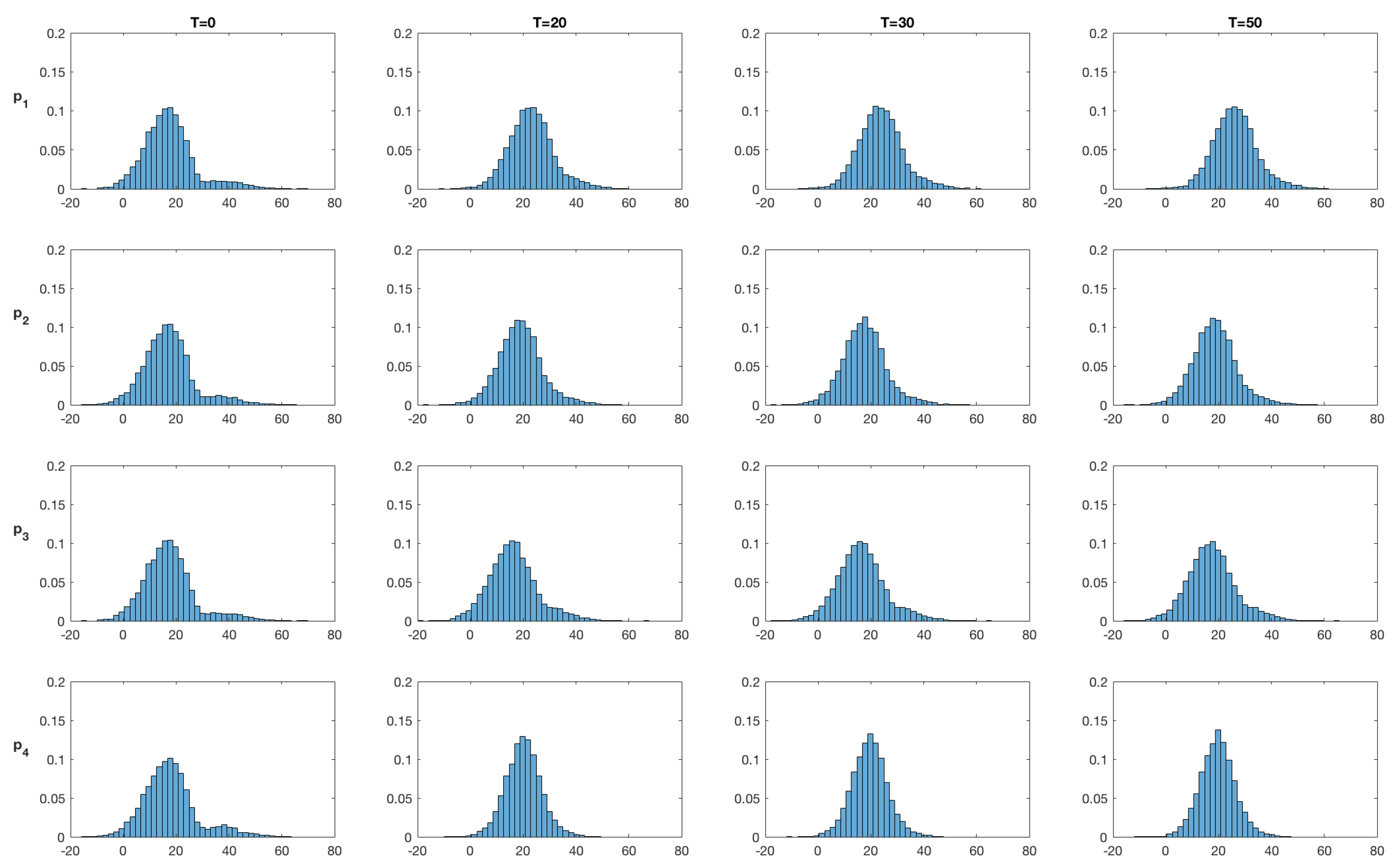
Figure 16.
SEnKS approach: Marginal posterior distributions of the initial temperature at time at monitoring locations () denoted (). The horizontal axes representing temperature are expressed in C.
Figure 16.
SEnKS approach: Marginal posterior distributions of the initial temperature at time at monitoring locations () denoted (). The horizontal axes representing temperature are expressed in C.
Figure 17.
EnKS approach: Marginal posterior distributions of the initial temperature at time at monitoring locations () denoted (). The horizontal axes representing temperature are expressed in C.
Figure 17.
EnKS approach: Marginal posterior distributions of the initial temperature at time at monitoring locations () denoted (). The horizontal axes representing temperature are expressed in C.
Figure 18.
MMAP predictions of the initial temperature (C) field at time for the SEnKS approach (upper) and the EnKS approach (lower).
Figure 18.
MMAP predictions of the initial temperature (C) field at time for the SEnKS approach (upper) and the EnKS approach (lower).
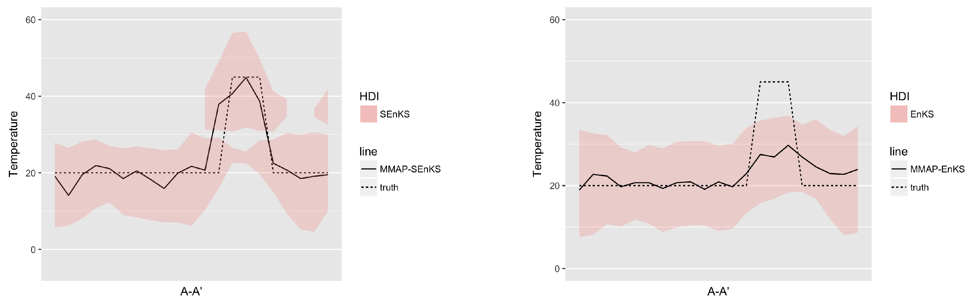
Figure 19.
MMAP predictions of the initial temperature (C) field with HDI in cross section A-A’ at time with SEnKS (left) and with EnKS (right).
Figure 19.
MMAP predictions of the initial temperature (C) field with HDI in cross section A-A’ at time with SEnKS (left) and with EnKS (right).
Figure 20.
SEnKS approach: Realizations from the posterior distribution of the initial temperature field at time . Upper panels: the colorbar gives the temperature in C. Lower panels: the horizontal axes represent the temperature (C), the vertical axes represent the relative prevalence of each temperature value for the realization right above.
Figure 21.
EnKS approach: Realizations from the posterior distribution of the initial temperature field at time . Upper panels: the colorbar gives the temperature in C. Lower panels: the horizontal axes represent the temperature (C), the vertical axes represent the relative prevalence of each temperature value for the realization right above.
Table 1.
Parameter values for the selection-Gaussian initial distribution for the initial log-diffusivity field.
Table 1.
Parameter values for the selection-Gaussian initial distribution for the initial log-diffusivity field.
| Parameters | Values |
|---|
| |
| 0 |
| |
| |
| A | |
Table 2.
RMSE comparing the MMAP prediction and the true log diffusivity field at time .
Table 2.
RMSE comparing the MMAP prediction and the true log diffusivity field at time .
| | SEnKF | ENKF |
|---|
| 2.72 | 3.76 |
Table 3.
Parameter values for the selection-Gaussian initial distribution for the initial temperature prior model.
Table 3.
Parameter values for the selection-Gaussian initial distribution for the initial temperature prior model.
| Parameters | Values |
|---|
| |
| 0 |
| |
| |
| A | |
Table 4.
RMSE comparing the MMAP prediction of the initial temperature field and the initial temperature field at time .
Table 4.
RMSE comparing the MMAP prediction of the initial temperature field and the initial temperature field at time .
| | SEnKS | ENKS |
|---|
| 2.92 | 3.72 |


