Behaviour of Uniform Drava River Sand in Drained Condition—A Critical State Approach

Abstract

Numerous triaxial tests on sand and sand-like materials have been performed worldwide during the past several decades. Their results provided a development of the advanced soil constitutive models and laboratory testing devices, as well as the establishment of a worldwide database of different types of uniform sandy materials. From such research, the critical state and steady state theory has emerged as one of the most useful tool for the modelling of a soil behaviour. This paper presents the results of static drained tests performed on the uniform Drava River sand from the Osijek region in Croatia. The main aim was to determine the shear behaviour and critical state, given that these characteristics are mostly unknown for the tested sand material. A series of detail triaxial tests were performed in drained conditions for three different initial relative densities, $D_R$, and two different loading directions; e.g., axial compression and axial extension. In total, 18 drained tests were performed. The study indicated that the value of ${33.75}^{\circ }$ is the critical friction angle for the tested sand. The relative density of 57% is determined as the critical relative density. Additionally, the study confirmed the difference in critical state for compression and extension loading. In addition, the results indicate that the sample preparation procedure has an important impact on the critical state of loosely prepared sandy samples. These results give the first insights into the behaviour of the Drava River sand, which can generally contribute to the worldwide sand behaviour knowledge base.

1. Introduction

One of the most useful tools and theories for the modelling of soil behaviour is the critical state and steady state theory [1,2,3,4,5,6,7]. The critical state theory has been a subject of soil investigation during the last several decades and was started with the research done by Casagrande [2]. As a theoretical framework, the critical state of soil was defined by Schofield and Wroth [5]. The critical state parameters have an important role in the geotechnical structure design, i.e., design of the stability of retaining walls, bearing capacity of spread foundation, etc. [8]. A soil, by definition, has reached its critical state when the shear strains ($\gamma$) or deviatoric strains (${ϵ}_q$) are developing without changes in mean effective stress ($p^{\prime }$), deviatoric stress (q) and specific volume (v). The critical state of a soil is such a state at which the plastic yielding can constantly develop without the change in deviatoric stress and specific volume at constant mean normal stress ($p^{\prime }$) [5,6,9]. Such yielding changes an initial soil fabric and structure, by destroying the initial contacts between the grains and rearranging them. Over the several past decades, there have been numerous research of triaxial tests on sand and sand-like materials. Extensive drained and undrained strength tests of uniform sands became an important research subject particularly after Niigata earthquake in 1964 [10,11]. The results lead to the development of the advanced soil constitutive models and laboratory testing devices, as well as to the establishment of a worldwide database of different types of uniform sandy materials.

Advanced drained and undrained triaxial tests and simple shear tests on uniform sands, which provided important insights into the critical state of sandy materials, have been performed on the Toyoura sand [12,13,14,15,16,17,18], Nevada sand [7,19,20], Ottawa sand [7,21,22,23], Monterey sand, e.g., [22,24,25,26] and Erksak sand, e.g., [9,27,28]. In addition to the fact that the above have established a database of the shear behaviour of uniform sands, they have also pointed out the difficulties and issues that may arise with the use of a triaxial device in laboratory research. Kang et al. [29] gave an overview of the main factors (i.e., sample size, particle size, void ratio and initial state) that can affect the behaviour of sand and its critical state.

In Eastern Croatia, which is a part of the European Pannonian Basin [30], uniform sands occur in the wider area of the City of Osijek. The City of Osijek is the largest economic centre of the Eastern Croatia and is the fourth largest city in Croatia, with a population of approximately 110,000. It is located on the right bank of the Drava River and has been constantly expanding in the last several years. The expansion of the city means that more and more geotechnical and structural work will take place on these uniform sandy deposits. Unfortunately, there is a lack of data on shear strength properties of this uniform sand. Several other cities and settlements are also situated close to the Drava River bank, on this type of sand. Cities such as Osijek are constantly widening with little or no knowledge of the soil material beneath. This type of sand has its use in constructions of sidewalks, as a fill material and a base for stone slab pavement or as a part of road construction [31,32,33]. The main aim of this study was to define critical state parameters of the uniform Drava River sand, by static drained triaxial tests. The sand was sampled in the area of Drava River bank, in the wider city centre of Osijek, from an excavation pit which is a part of Osijek Port Tranzit complex. Beside the critical state parameters, physical properties of the Drava River sand (i.e., specific gravity, grain size distribution, minimum and maximum void ratio) are also determined in this study. The findings from this study certainly contribute to the general knowledge of the sand materials in the studied area, as well as to the behaviour of uniform sandy materials in drained condition. This will also allow using Drava River sand, as a locally available sand, in preparation of small-scale models for experimental studies of soil-structure interaction.

2. Physical Properties of Tested Material

2.1. Origin of Drava River Sands

The Drava River sand tested in this study originates from the wider area of the City of Osijek, located in Eastern Croatia, which is a part of the European Pannonian Basin [30]. The City of Osijek belongs to the Drava depression zone, characterized by the lowland relief and complex geological settings [34]. The city area is predominantly composed of heterogeneous mixtures of Quaternary deposits, among which the Pleistocene continental, marshy and lacustrine loess sediments and Holocene Drava River terrace sediments are generally distinguished. The Drava River sand belongs to the multiphase flooded lithological complex of the Holocene terrace, formed at the right bank of the Drava River. The thickness of the river terrace sediments ranges between 2 and 6 m, and the maximum terrace width is approximately 3.3 km [34]. Sands and sandy silts prevail, with subordinate silty clays. Quartz (approx. 50%), feldspar (approx. 25%) and carbonates (approx. 25%) are the main minerals in the sands, with subordinate muscovite and rock fragments. A high magnification image of tested sand was made and presented in Figure 1, magnified 30 times. For this purpose, an EOL scanning electron microscope with maximum resolution of 0.8 nm was used with the acceleration charge of 10 kV and working distance of 10 mm [35,36]. It can be observed that the tested sand is generally characterized by the uniformity of particle shape, which are predominantly of low sphericity and angular to subangular [37].

The main physical properties of soil, such as, specific gravity, particle size distribution, minimum and maximum void ratios of this sand type were tested and are presented in the following subsections.

2.2. Specific Gravity

The specific gravity of tested material is 2.66. The value is very similar to sands such as Monterey No. 0 sand, e.g., [22,26] and Ottawa sand, e.g., [21,22],

Table 1. Basic mechanical properties of various type of sands.

Sand Types	${\mathit{G}}_{\mathit{s}}$	${\mathit{C}}_{\mathit{u}}$	${\mathit{C}}_{\mathit{c}}$	${\mathit{D}}_{50}$	${\mathit{D}}_{10}$	${\mathit{e}}_{\mathit{max}}$	${\mathit{e}}_{\mathit{min}}$
DrOS018	2.66	1.67	1.07	0.28	0.18	0.951	0.627
Toyoura [12,13,14,18]	2.65	1.29–1.7	1–1.07	0.17–0.21	−0.16	0.977–0.992	0.597–0.632
Nevada [7,19,20]	2.67	1.22–2.31	0.89–1.02	0.16–0.21	0.08–0.18	0.858–0.887	0.511–0.581
Monterey [22,25]	2.65	1.28–1.5	0.99–1	0.35–0.36	0.26–0.3	0.85–0.86	0.55–0.56
Ottawa [7,21,22,23]	2.64–2.67	1.18–1.73	0.96–1.26	0.17–0.7	0.12–0.6	0.67–0.83	0.46–0.51

. Specific gravity test was performed according to the European standard for identification and classification of soil [38]. The tests using both vacuum procedure and boiling technique were performed.

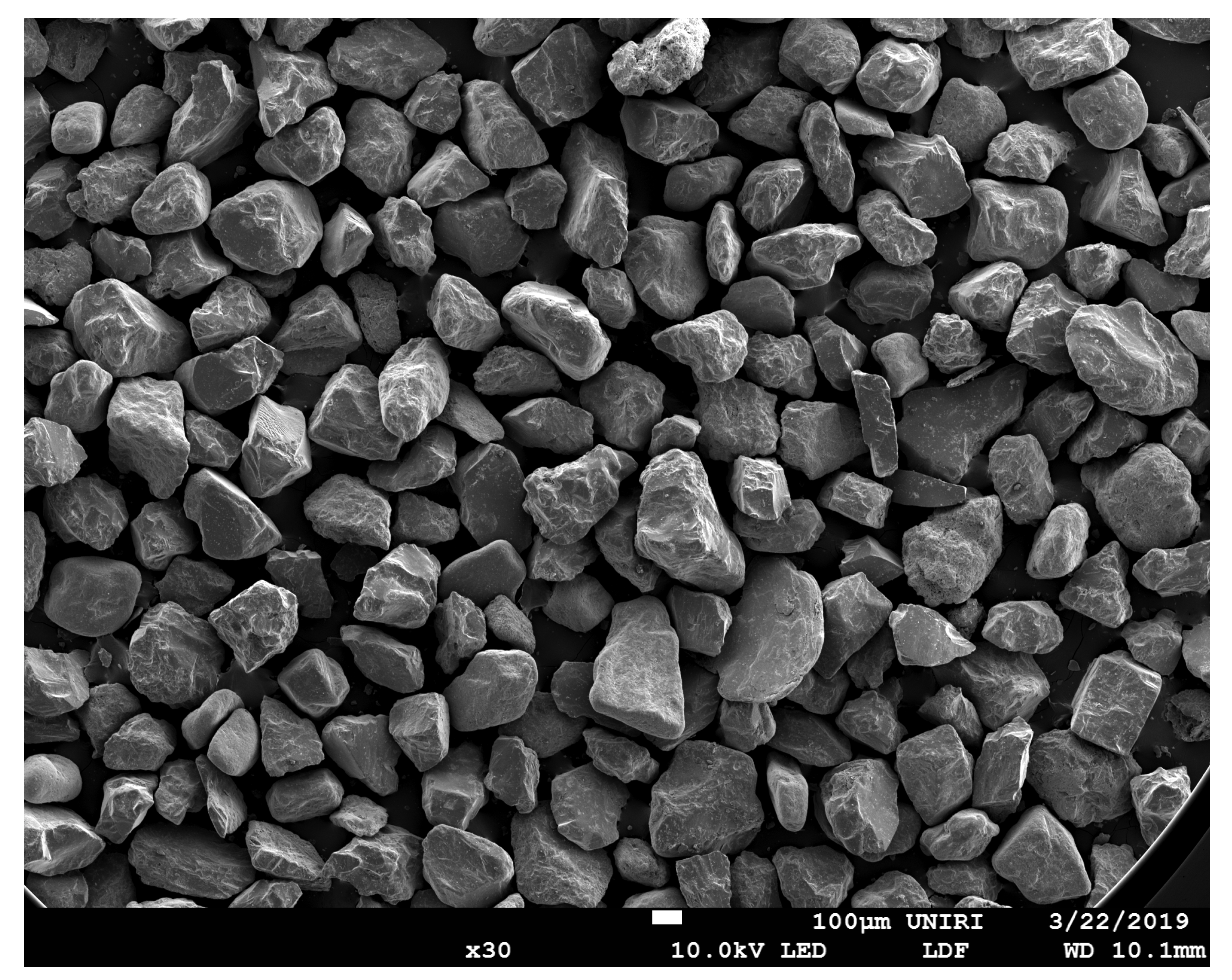
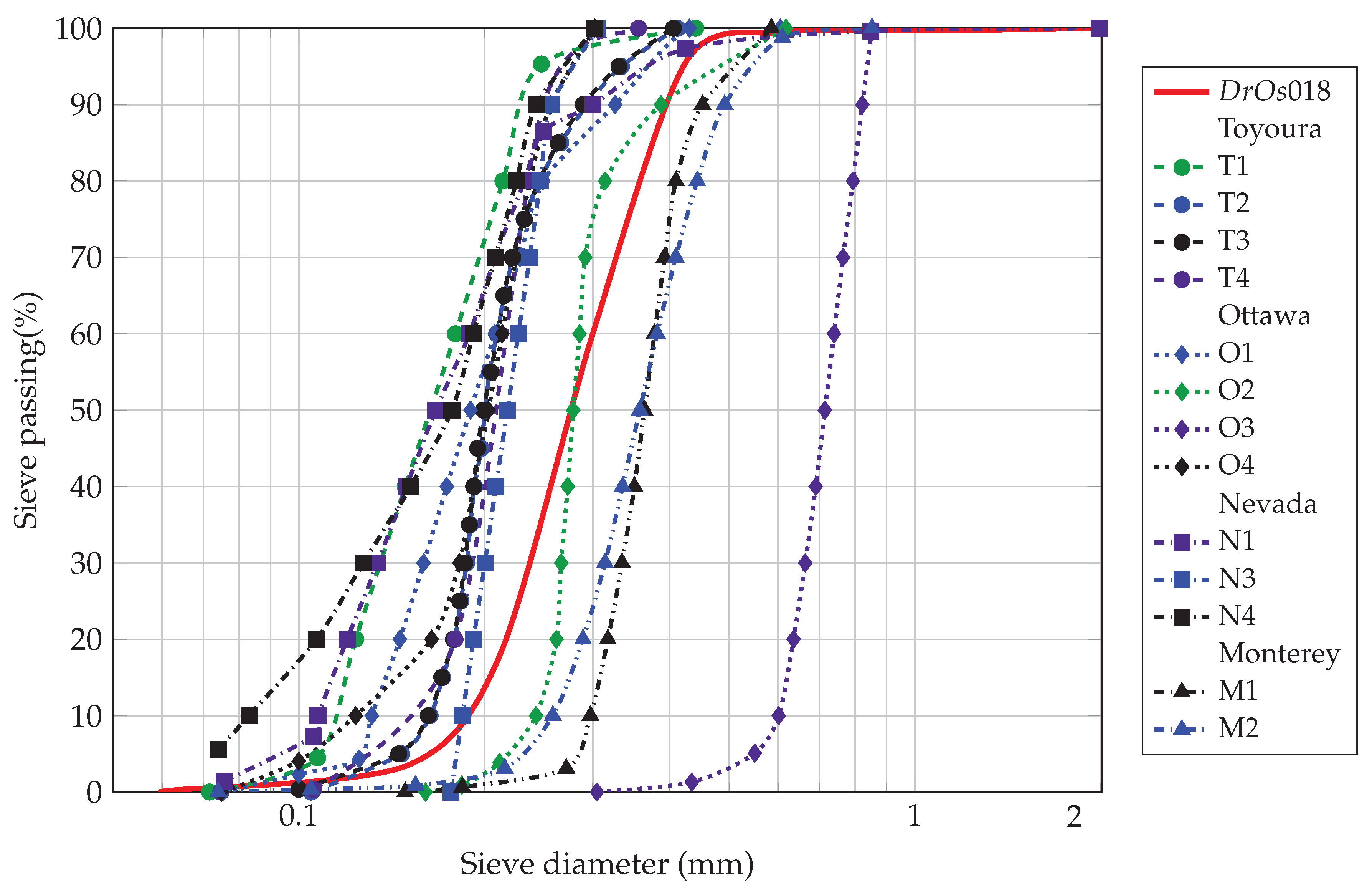
2.3. Grain Size Distribution

The tested Drava River sand represents a uniformly graded sand (Figure 2). The sieve analysis was performed according to the European standards [39], and results are plotted in comparison to the similar sand type materials listed in Table 1. The mean grain size diameter ($D_{50}$) is approximately 0.28 mm, and the effective grain diameter ($D_{10}$) is 0.18 mm. The coefficient of curvature $C_u$ is approximately 1.67, which is more than a half of the value of uniformity limit ($C_u>4$ for sand to be nonuniform). Given that tested sand has never been assigned by the name or designation, the authors used the abbreviation of “DrOS018” to name the specific sand. In abbreviation, the first two letters are associated to sand’s origin and geographical setting (i.e., Drava River and City of Osijek), while the numbers are associated to the effective diameter of grain size (i.e., $D_{10}=0.18$ mm).

2.4. Minimum and Maximum Density

The minimum void ratio ($e_{min}$) and maximum void ratio ($e_{max}$) of tested sand are 0.627 and 0.951, respectively. The obtained values of minimum and maximum void ratio are compared with the similar uniform sands from literature and presented with Table 1. Values of minimum and maximum void ratios are determined in two ways, (i) using vibration table, according to ASTM standard [40] and (ii) using the vibration type sieve shaker. For the vibratory table technique, split mould defined with ASTM standard [40] was used. For the second method, using vibration sieve shaker, two-part mould of 150 mm in diameter, which is usually common for Proctor’s compaction test, was used for this purpose. The applied method here was modified based on the ASTM standard for standard test methods for maximum index density using a vibratory table [41]. The sand was loaded with the surcharge weight of 10 kg and let to vibrate for 10 min. From the simple phase relation of a soil element [42,43] and using the ASTM standard for minimum and maximum void ratio [40], the void ratio can be expressed as a function of specific gravity and dry unit density Equation (1). The difference in void ratio using a vibratory table technique mentioned above was 0.3% which can lead to the conclusion that the modified machine such as vibration sieve shaker can be used for determination of minimum void ratio.

$$e_{\square }=\frac{G_s}{{\rho }_{d,\square }}·{\rho }_w-1$$

(1)

where ($G_s$) is specific gravity of sand, (${\rho }_d$) is dry density of soil and ($\square$) stands for “min” or “max”, depending on the type of density used in calculations.

As for maximum void ratio and its minimum relative density, the value was determinate in three ways, using the same methodology. The value was determinate by pouring the sand in three different moulds: (i) fall cone cup, (ii) 38 mm in diameter triaxial sample cutter and (iii) proctor mould 101 mm in diameter. Fall cone cup and triaxial sample cutter gave similar results, with the difference in less than 0.1%. Fall cone cup resulted in the value of 0.952 and the triaxial cutter in value of 0.951. Proctor’s 101 mm diameter mould gave a value of maximum void ratio equal to 0.949, which is 0.2% smaller in comparison with the value obtained by triaxial cutter, which can be caused because of surcharge load. Taking the average of these three values results in the maximum value of void ratio ($e_{max}=0.951$).

3. Tests Equipment and Procedures

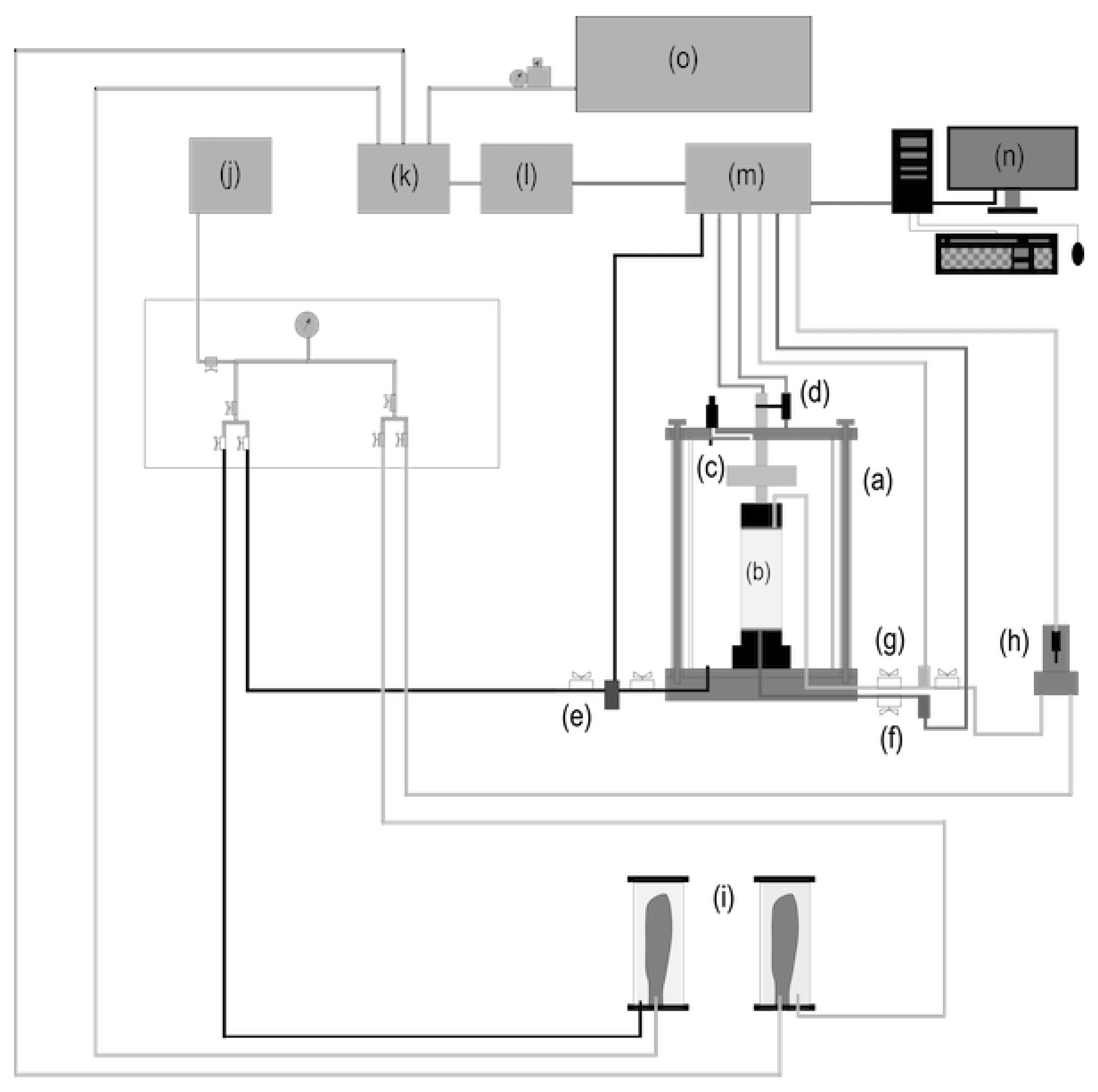
3.1. Triaxial Test Apparatus

Fully automated triaxial system was used for static drain tests on described type of sand. All tests were performed in the Geotechnical laboratory at the Faculty of Civil Engineering, University of Rijeka, equipped with triaxial system manufactured by Wyckeham Farrance, Controls Group srl [44]. The equipment consists of a computer-controlled system that provides easy test performance. The experiments were conducted using a loading frame, with the capacity of 50 kN. The capacity of triaxial cell was 2500 kPa, and the capacity of the load cell used for performed tests was 25 kN. Submerged type of load cell was used in all of the tests. Figure 3 presents the schematic view of a used triaxial system.

Tests were performed according to the ASTM standard for consolidated drained triaxial test [45]. Axial strain was calculated as a ratio between the vertical displacement ($\mathsf{\Delta }$) measured with vertical displacement transducer (LVDT) (Figure 3d) and sample height after consolidation ($H_c$). The vertical stress was calculated as a ratio of measured force in load cell (Figure 3c) and corrected sample area, (A) (Equation (2)). Volumetric change was measured using the volume change device (Figure 3h). Membrane corrections were taken into account as recommended by ASTM standard [45] and Lade [46]. Radial displacements could not be measured due to lack of measuring equipment.

$$A=A_0·\frac{1-{ϵ}_v}{1-{ϵ}_a}$$

(2)

where $A_0$ is the initial area of sample after consolidation, ${ϵ}_v$ is the volumetric deformation and ${ϵ}_a$ is the axial deformation.

The main advantage of triaxial system is its simplicity and modularity. The main issue is the possible contact loss during saturation and consolidation stage, usually controlled by PID controller tab within operating software. The PID stands for Proportional/Integrate/Derivative controller options within an integrated closed loop system, e.g., [47]. This issue can happen during long periods of saturation and consolidation, which is possible during tests on clay material. In this research such events were seldom, but there has been some indication of such system behaviour while conducting extension tests. To avoid the issues regarding the sample size, all the tests were performed on the 70 mm diameter sample. As it was mentioned earlier, the sample size has a significant effect to critical state [48].

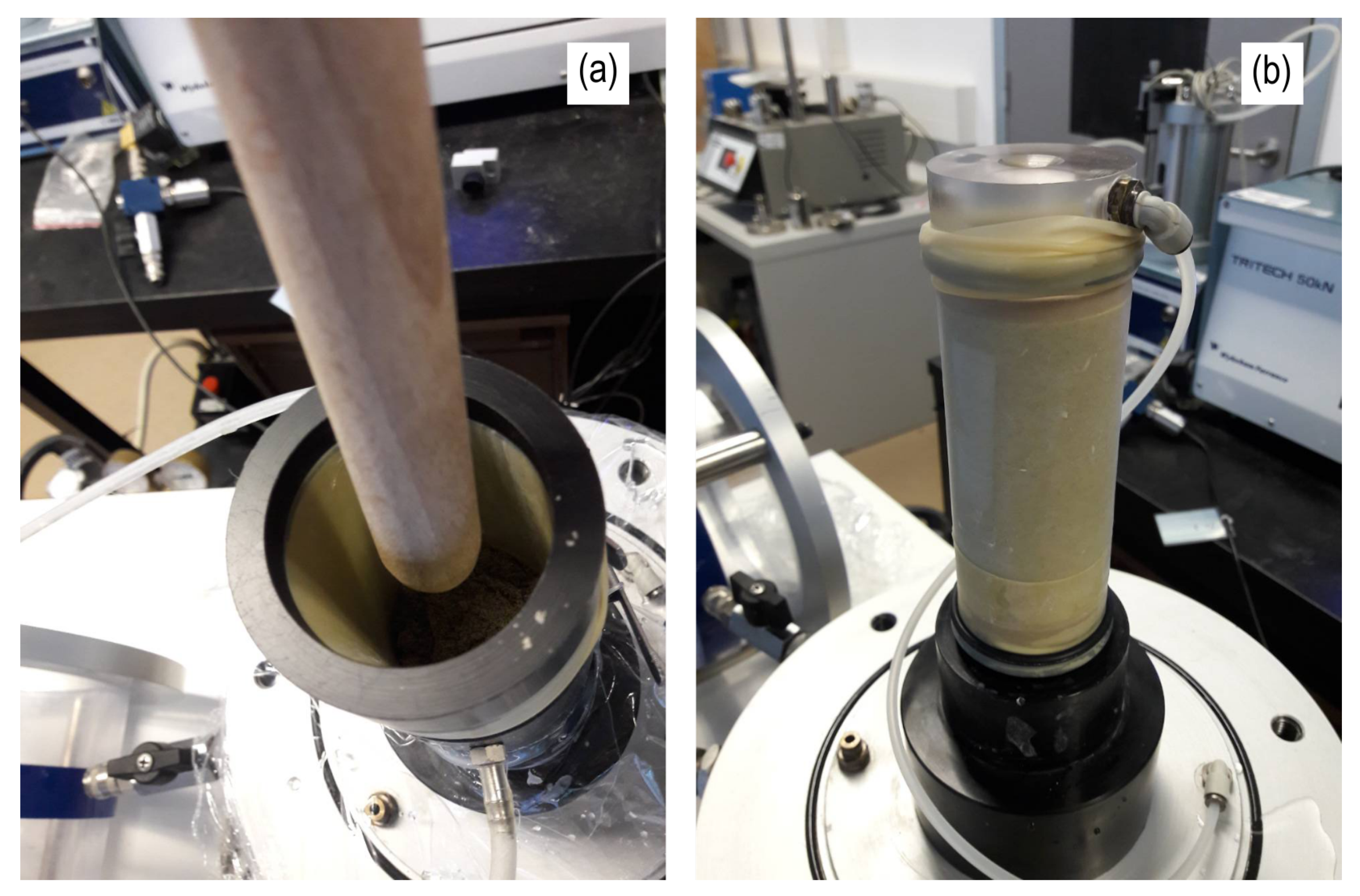
3.2. Sample Preparation

As it is specified in

Table 2. Summary of performed tests.

Test Number	Test ID	Effective Confining Stress, ${\mathit{p}}_0^{\prime }$ (kPa)	Relative Density, ${\mathit{D}}_{\mathit{R}}$ (%)	Loading Type
1	049C10033DRN	100	33	Compression
2	056C20033DRN	200
3	055C40033DRN	400
4	044E10033DRN	100		Extension
5	045E20033DRN	200
6	047E40033DRN	400
7	040C10050DRN	100	50	Compression
8	039C20050DRN	200
9	005C40050DRN	400
10	008E10050DRN	100		Extension
11	012E20050DRN	200
12	048E40050DRN	400
13	007C10080DRN	100	80	Compression
14	009C20080DRN	200
15	011C40080DRN	400
16	016E10080DRN	100		Extension
17	017E10080DRN	200
18	018E40080DRN	400

, specimens at three different densities were tested in this research. To achieve comparable results, the undercompaction method in specimen’s preparation was employed. The method was developed by Ladd [49] and provides continuous density throughout the sample height and it was used in laboratory tests very often. The method ensures repeatable test results, minimizes particle segregation and offers a preparation of reconstituted sand specimen, [49]. Figure 4 presents the specimen preparation using undercompaction method (Figure 4a) and prepared specimen for drained compression test (Figure 4b). The diameter of a compaction rod was 1 cm and was made of a hard wood. This ensured the best control of energy used for compaction and reduced the possibility of grain crushing during compaction process.

The authors are well aware that the method can produce some effects on the initial state, which in turn can have influence on critical state, [9,50,51,52]. Nevertheless, the method is used mainly because of the repeatability of the sample preparation. Before the start of main test stage, several tests were performed under different undercompaction degree, as suggested by several authors [1,46,49]. It has been found that the optimal value of undercompaction degree is between 4 and 5%. The authors used the value of 5% for the undercompaction degree in this research. Besides initial tests performed to establish a degree of undercompaction, several tests were also performed to define the optimum number of the undercompaction layer. During the initial tests, it has been found out that the optimum number of layers is around 15 layers. Several tests were performed in order to take into account the different initial water content during undercompaction preparation. The water content used for preparation was found to be the best at 3.5%. At lower water content the sand was relatively dry, thus limiting the grain-to-grain sliding, while at higher water content the sand grains were able to easily slide of one another due to water film developed around soil particles [42], making it harder to finish the top layer during specimen preparation. This showed some issues during initial testing, especially in extension tests, in the view of “necking” in the upper part of the specimen (near the top cap), which can in turn lead to nonuniform density distribution throughout a specimen. The height of each layer was controlled using a standard laboratory caliper. Tamping of each layer was performed using wood stopper with the edges slightly rounded in order to reduce possible damages to the latex membrane. Each layer was compacted by 10 blows.

3.3. Testing Program

Series of detail triaxial tests were performed on fine sand in drained conditions. Summary of prepared samples are presented in Table 2. Sand samples were prepared under three different initial relative densities, ($D_R$), thus having loose, medium dense and dense condition of relative density. Tests were performed under two different loading directions: (i) axial compression and (ii) axial extension.

To reach the maximal saturation, increments of back pressure were applied in the saturation stage. Prior to the saturation stage, samples were flushed by (CO₂) approximately 15 to 30 min, depending on initial sample density and suggestions from the literature [46,53]. To reach maximal saturation utilising lower values of back pressure, the specimens are then percolated with deaired water taking care at the effective stress during percolation. As stated earlier, the saturation was performed in several stages by increasing back pressure. The degree of saturation was monitored using Skempton’s B coefficient [46]. Because of (CO₂) flushing and water percolation, the values of back pressure, at which B value higher than 0.98 were reached, were around 90 kPa. Samples were isotropically consolidated at the defined effective consolidation stress as it is presented in Table 2. Consolidation was performed in several stages, gradually increasing effective confining stress, in order to reduce a possibility of high values of hydraulic gradient during water outflow. For example, if a specimen had to be consolidated on effective stress of 100 kPa, it was previously consolidated on effective stresses 25, 50 and 75 kPa. Mentioned technique of slow drainage valve opening, with the combination of several consolidation stages, leads to safe and successful consolidation of a specimen to the planned effective consolidation stress. Described consolidation procedure means that the rate of shearing could not be calculated directly form the consolidation stage. Taking that into account, several tests were performed during initial testing in a regular manner, that is without the valve regulation, mentioned in the earlier section (Section 3.2). The results of these tests are not presented in this paper, as they were used to obtain the proper strain rate loading. These tests resulted in a calculated average axial strain rate of 4% per hour on average. Based on the response of the specimens in these initial tests, a straining rate of 4% axial strain per hour was used throughout the shearing stages of both compression and extension type of tests. The results of performed static drained tests are presented in the following section.

4. Results of Laboratory Tests

Results of drained triaxial tests for loose, medium dense and dense Drava River sand are presented in Figure 5, Figure 6 and Figure 7, respectively. Figure 5a, Figure 6a and Figure 7a present the effective stress paths in ($p^{\prime }-q$) plane for both compression and extension tests. The mean effective stress is calculated based on the Equation (3) and deviatoric stress is calculated based on the Equation (4).

$$p^{\prime }=\frac{{\sigma }_a^{\prime }+2·{\sigma }_r^{\prime }}{3}$$

(3)

$$q={\sigma }_a^{\prime }-{\sigma }_r^{\prime }$$

(4)

where ${\sigma }_a^{\prime }$ is the effective axial stress, and ${\sigma }_r^{\prime }$ is effective radial stress.

Proposed failure and critical lines are also presented in the same plots, defined with the M sign. Indices C and E present corresponding lines in compression and extension, while symbols f and cs note for failure and critical state, respectively. Stress-strain behaviour for both compression and extension types of tests are presented in Figure 5b, Figure 6b and Figure 7b. Deviator stress (q) is plotted against relative axial strain (${ϵ}_a$). The variation of specific volume (v) with mean effective stress ($p^{\prime }$) are plotted in Figure 5c, Figure 6c and Figure 7c. The values of the strength ratios in compression and extension, along with effective friction angle are presented in

Table 3. Summary strength parameters.

Relative Tensity, ${\mathit{D}}_{\mathit{r}}$ $(\%)$	${\mathit{M}}_{\mathit{C},\mathit{f}}$	${\mathit{M}}_{\mathit{E},\mathit{f}}$	${\mathit{M}}_{\mathit{C},\mathbf{cs}}$	${\mathit{M}}_{\mathit{E},\mathbf{cs}}$	${\mathit{\varphi }}_{\mathit{C},\mathbf{peak}}^{\prime }$	${\mathit{\varphi }}_{\mathit{E},\mathbf{peak}}^{\prime }$	${\mathit{\varphi }}_{\mathit{C},\mathbf{cs}}^{\prime }$	${\mathit{\varphi }}_{\mathit{E},\mathbf{cs}}^{\prime }$
33	1.3349	0.936	1.3109	0.9221	33.09	33.68	32.54	33.01
50	1.3547	0.9541	1.2326	0.7657	33.54	34.56	30.75	26.03
80	1.4468	1.0443	1.2114	0.7113	35.65	39.21	30.26	23.79

. These values are based on Figure 5a, Figure 6a and Figure 7a.

Values of specific volume after consolidation stage and after shearing stage are approximated with the curve rather than a line, as suggested by Been et al. [9] using the Equation (5).

Fit parameters were determined as nonlinear fit model parameters based on the nonlinear regression algorithm [54,55,56] with the assumed shape of the fit function that corresponds to the Equation (5).The thick line presents the isotropic consolidation curve, while the dashed line presents the critical state curve. Values of the fit parameters from Equation (5) are presented in

Table 4. Summary of Equation (4) fit parameters.

Relative Density, ${\mathit{D}}_{\mathit{r}}$ $(\%)$	${\mathit{\Gamma }}_{\mathit{c}}$	${\mathit{\lambda }}_{\mathit{c}}$	${\mathit{\kappa }}_{\mathit{c}}$	${\mathit{\Gamma }}_{\mathbf{CS}}$	${\mathit{\lambda }}_{\mathbf{CS}}$	${\mathit{\kappa }}_{\mathbf{CS}}$
33	1.844	0.016	0.7	1.80	0.016	0.7
50	1.789	0.02	0.7	1.775	0.02	0.7
80	1.692	0.016	0.7	1.725	0.016	0.7

and can be used as an input parameter for simple numerical analysis. The change in specific volume (v) related to relative axial deformation (${ϵ}_a$) are plotted on Figure 5d, Figure 6d and Figure 7d. Stress-strain behaviour for both compression and extension types of tests are presented in Figure 5b, Figure 6b and Figure 7b. Deviator stress q is plotted against relative axial strain ${ϵ}_a$. The variation of specific volume $\left(v\right)$ with mean effective stress $\left(p^{\prime }\right)$ is plotted in Figure 5c, Figure 6c and Figure 7c. Values of specific volume after consolidation stage and after shearing stage are approximated with the curve rather than a line, as suggested by Been et al. [9] using the Equation (5). The thick line presents the isotropic consolidation curve, while the dashed line presents the critical state curve. Values of the fit parameters from Equation (5) are presented in Table 4 and can be used as an input parameter for simple numerical analysis. The changes in specific volume $\left(v\right)$ related to relative axial deformation $\left({ϵ}_a\right)$ are plotted on Figure 5d, Figure 6d and Figure 7d.

$$v=\mathsf{\Gamma }-\lambda ·{\left(\frac{p^{\prime }}{p_a}\right)}^{\kappa }$$

(5)

where v is the specific volume, $\mathsf{\Gamma }$ is the value of specific volume at $p^{\prime }$ = 1 kPa, $p^{\prime }$ is the mean effective stress, $p_a$ is the atmospheric pressure of 101.25 kPa and $\kappa$ is the exponent factor.

From the presented compression and extension tests, the elastic soil parameters were determined,

Table 5. Elastic modulus of performed tests.

Relative Density ${\mathit{D}}_{\mathit{R}}$ [%]	Confining Pressure ${\mathit{\sigma }}_{\mathit{c}}^{\prime }$ [kPa]	Test Type *	Young Modulus $\mathit{E}$ [kPa]	Shear Modulus $\mathit{G}$ [kPa]	Bulk Modulus $\mathit{K}$ [kPa]	Poisson Ratio $\mathit{\nu }$
33	100	C	40,772	16,394	26,494	0.24
33	200		76,935	30,995	49,527	0.24
33	400		126,870	52,567	72,107	0.21
50	100		25,511	10,253	16,612	0.24
50	200		57,736	23,492	35,486	0.23
50	400		76,618	30,880	49,220	0.24
80	100		36,739	14,769	23,898	0.24
80	200		52,652	21,177	34,168	0.24
80	400		105,298	44,292	56,370	0.19
33	100	E	37,283	16,553	16,624	0.13
33	200		58,768	22,632	48,570	0.30
33	400		124,151	45,362	157,277	0.37
50	100		27,508	10,555	23,277	0.30
50	200		93,624	35,578	84,701	0.32
50	400		235,196	93,098	165,511	0.26
80	100		44,685	16,680	46,405	0.34
80	200		106,226	42,662	69,423	0.24
80	400			219,668	77,520	440,288	0.42

[*] C—compression; E—Extension.

.

From the presented compression and extension tests, elastic soil parameters were determined. Values obtained are summarised in Table 5.

The values for Young modulus (E) were obtained during the stress-strain ratios from Figure 5b, Figure 6b and Figure 7b based on a general relation between deviatoric stress (q) and axial strain (${ϵ}_a$), Equation (6). The shear modulus was calculated using the relation between deviatoric stress and deviatoric strain, [6], (Equation (7)). The plots of deviatorc stress and deviatorc strain are not presented here. Poisson ration ($\nu$) was calculated based on the relation between axial strain and volumetric strain (${ϵ}_v$), (Equation (8)), while the bulk modulus was calculated using the values of Young modulus (E) and Poisson’s ratio ($\nu$). The values of strength ratio in compression and extension, along with effective friction angle are presented in Table 3. These values are based on Figure 5a, Figure 6a and Figure 7a, as described earlier.

$$E=\frac{q}{{ϵ}_a}$$

(6)

$$G=\frac{q}{{ϵ}_q}$$

(7)

$$\nu =\frac{{ϵ}_v}{{ϵ}_a}$$

(8)

The data from Figure 5c, Figure 6c and Figure 7c are plotted in Figure 8 where filled square marks present the values of specific volume $\left(v\right)$ after isotropic consolidation stage while the empty square marks present the specific volume at the assumed critical state. Densely dotted curves are presenting the isotropic consolidation curves, while the dashed curve present the critical state.

The data in Figure 8 present a tendency toward a critical state. The data from Figure 9 is plotted using the power low given with Equation (5), [57]. The exponent $\kappa$ is used as a best fit parameter, which is determined based on the data in Table 4. The data are presented in Figure 9. The upper and lower bound of critical state can easily be defined as well as the best approximation of critical state line (approximated dashed line).

Upper and lower bound lines, together with critical state line were then transferred back to standard $v-log{p}^{\prime }$ plane, which is plotted once again in Figure 10. From this figure it can be easily noticed that the critical state is very close to the critical state obtained by medium dense samples. The relative density $\left(D_r\right)$ which corresponds to those value of voids e is approximately 57%.

Since critical state could not be uniquely defined, authors have analysed plastic dilatancy for the DrOS018 sand. Stress dilatancy was calculated as suggested by Been and Jefferies [28] and Azeiterio et al. [58]. Plastic dilatancy was calculated using Equation (9). Values of elastic shear and bulk modulus were calculated based on the initial data reading of tests (Table 5), which is proven valid in some earlier research (for example, [28,58,59]). Plastic dilatancy (Equation (9)) was calculated only for compression tests for all three different initial densities and it was calculated and plotted against the stress ratio $\eta$ (Equation (10)).

$$D^p=\frac{d{ϵ}_v^p}{d{ϵ}_q^p}\approx \frac{\left({ϵ}_{v_{j+1}}-{ϵ}_{v_j}\right)-\left(p_{j+1}^{\prime }-p_j^{\prime }\right)/K}{\left({ϵ}_{q_{j+1}}-{ϵ}_{q_j}\right)-\left(q_{j+1}-q_j\right)/3G}$$

(9)

where ($d{ϵ}_v^p$) is the increment of plastic volumetric deformation, ($d{ϵ}_p^p$) is the increment of plastic deviatoric deformation, (${ϵ}_{v_{j+1}}-{ϵ}_{v_j}$) forward difference in total volumetric deformation, (${ϵ}_{q_{j+1}}-{ϵ}_{q_j}$) forward difference in total deviatoric deformation, ($\frac{p_{j+1}^{\prime }-p_j^{\prime }}{K}$) forward difference in elastic volumetric deformation and ($\frac{q_{j+1}^{\prime }-q_j^{\prime }}{3G}$) forward difference in elastic deviatoric deformation.

$$\eta =\frac{q}{p^{\prime }}$$

(10)

where q is deviatoric stress and $p^{\prime }$ mean effective stress.

Figure 11, Figure 12 and Figure 13 correspond to the initial densities of 33%, 50% and 80%, respectively.

It can be identified a small negative plastic dilatancy for loose sample, indicating that the sample could exhibit small dilatative behaviour. Critical state stress can be found if the maximum stress ratio ${\eta }_{max}$ is plotted against the minimum plastic dilatancy $D_{min}$, as proposed by Vaid and Sasitharan [60] and Been and Jefferies [28]. Scatter plot in Figure 14 presents the relationship between the two mentioned parameters. According to Nova and Wood [61] and Jefferies and Shuttle [62], the data can be approximated with the Equation (11) and $N=0$ which leads to the critical stress ratio M of 1.364 and equivalent effective angle of friction ${\varphi }_c={33.75}^{\circ }$:

$${\eta }_{max}=M-\left(1-N\right)·D_{min}^p$$

(11)

where ${\eta }_{max}$ is maximum stress ratio, M is a critical friction ratio, N volumetric coupling parameter and $D_{min}^p$ minimum plastic dilatancy.

In Figure 14 the values of minimum plastic dilatancy and maximum stress ratio are plotted and compared with the data obtained from literature. Approximation lines for the volumetric coupling parameter equal to $N=0$ and $N=M/3$ [63] are compared as well.

With the critical state approximated and assumed, the state parameter ${\psi }_0$ can now be calculated next, as defined by Been and Jefferies [27] and Jefferies [64], Equation (12).

$${\psi }_0=e_c-e_{CS}$$

(12)

where $e_c$ presents the void ratio after consolidation, and $e_{CS}$ present the void ratio at critical state.

Values of state parameter are plotted related to the peak friction angle (Figure 15) and against the volumetric strain at the peak friction angle (Figure 16). The shaded part of the figures present the range of data from various tests [60,62,65].

5. Discussion

A series of drained triaxial tests under three different initial states were conducted on Drava River sand. The results consist of simple stress-strain relation, change in volume behaviour and plastic dilatancy relations.

Basic stress-strain relation with volume behaviour was presented in Figure 5, Figure 6 and Figure 7, for loose, medium dense and dense samples, respectively. The results for densely prepared sand samples show an expected behaviour. There is a significant difference in peak and residual deviatoric stress $\left(q\right)$ as can be depicted form Figure 7b. The approximated isotropic consolidation curve fits well on consolidated data for both extension and compression test. As it is mentioned before, extension tests cannot reach the same critical state as compression tests, but the results show the tendency toward the dashed critical state curve, Figure 7c. From Figure 7d it can be concluded that all six samples have reached the critical state.

Critical state values of DrOS018 sand form a relatively narrow range of specific volume variation, as presented in Figure 8. The average difference in specific volume is from 0.0395, for large confining stress, to 0.0365 for low confining stress. This is very similar to the data presented by Been and Jefferies [28]. As mentioned before, the data of specific volume were plotted against normalised mean effective stress with atmospheric pressure, Figure 9. The type of plot presented in Figure 9 ensured the smallest error in the critical state range and was used to propose the best fit parameters for critical state of DrOS018 sand, Figure 10. Comparing the Figure 8 and Figure 10 it is quite noticeable that the proposed critical state is very close to the isotropic consolidation curve for the samples with 50% initial relative density. This is one of the reasons why the results in that area show versatile results. In order to define a critical state parameter M, and thus the critical friction angel ${\varphi }_{cs}^{\prime }$, plastic dilatancy was calculated, which are plotted for loose, medium dense and dense samples on Figure 11, Figure 12 and Figure 13, respectively. Figure 12 and Figure 13 indicate that the value of critical state parameter is somewhere between 1.3 and 1.4. This was confirmed by plotting the maximum values of stress ratio ${\eta }_{max}$ against the minimum plastic dilatancy $D_{min}^p$, Figure 14. The data were approximated with the line whose slope represents the critical state parameter M, that equals 1.364. This indicates that the critical state friction angle for DrOS018 is ${33.75}^{\circ }$. Figure 14 also shows the data compared with the test presented by Vaid and Sasitharan [60] and Cornforth [65]. The data obtained from this research are in the range of Vaid and Sasitharan’s data for negative plastic dilatancy but with smaller slope. Further investigations will be made with the focus on the slope of plastic dilatancy to maximum stress ratio. Data for Cornforth [65] were modified according to [64]. Values of peak friction angle (${\varphi }_{peak}$) and state parameter (${\psi }_0$) were plotted together and compared with the range of various tests, Figure 15. Although there is a small discrepancy in data, it is visibly a clear and valid trend of how the friction angle changes with the change of state parameter. The concerning part is that the tested data are in the upper bound of all documented data, according to Jefferies [64]. Further investigations will be performed to refine those points. The values of state parameter compared to the volumetric strain at peak friction angle, as presented on Figure 16, are in good agreement with the previously tested sands [64].

6. Conclusions

A series of detail triaxial tests were performed on sand in drained conditions under three different initial relative densities, $D_R$. The tests were performed under two different loading directions: axial compression and axial extension, in total 18 drained tests. The test provided a first insight into the behaviour of Drava sand from Osijek region of such kind. Results of the performed tests show some minor discrepancies, probably due to testing equipment, but are in good agreement with the tests on similar materials documented in literature. Based on the results and discussion above, it can be concluded:

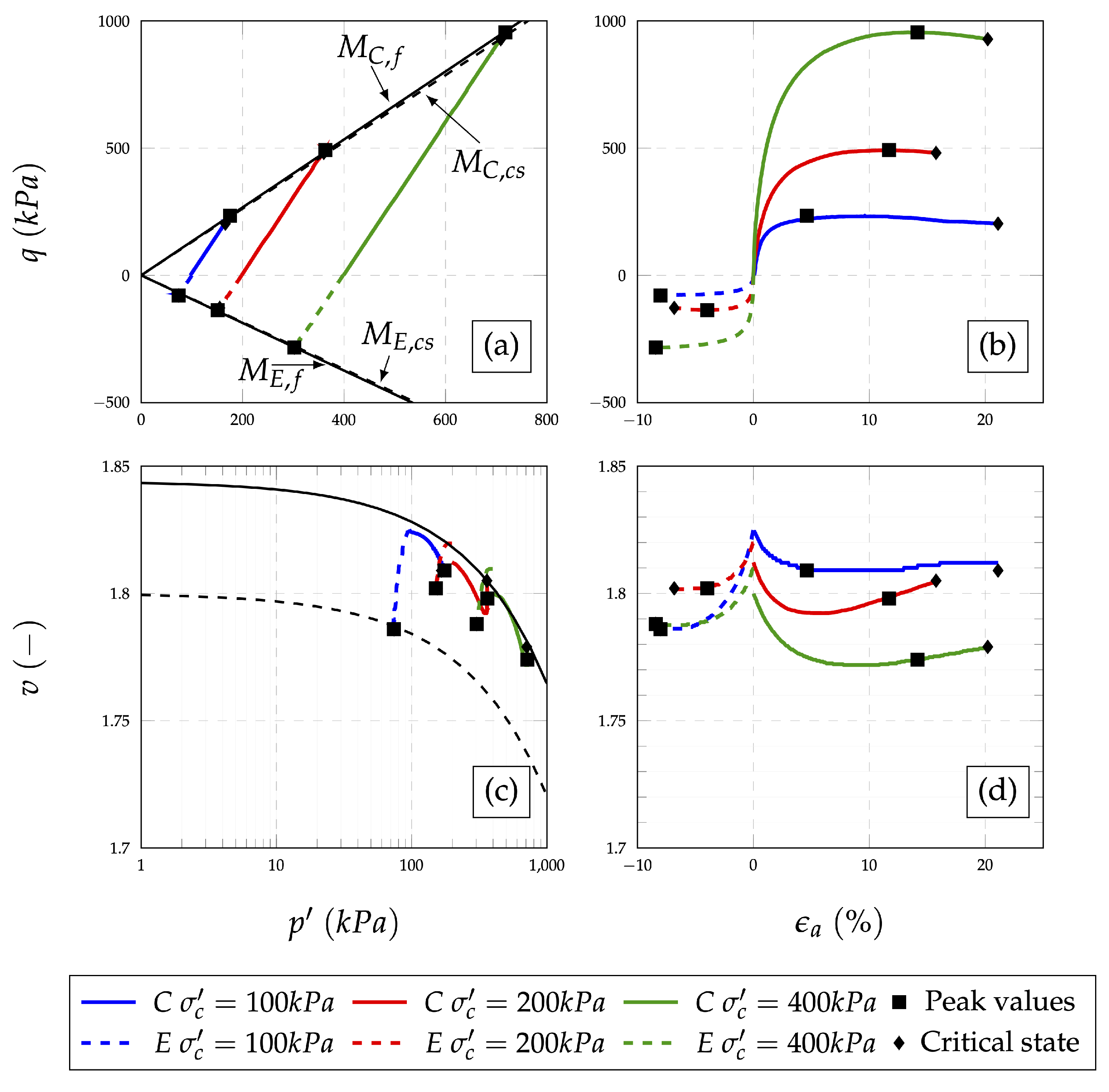
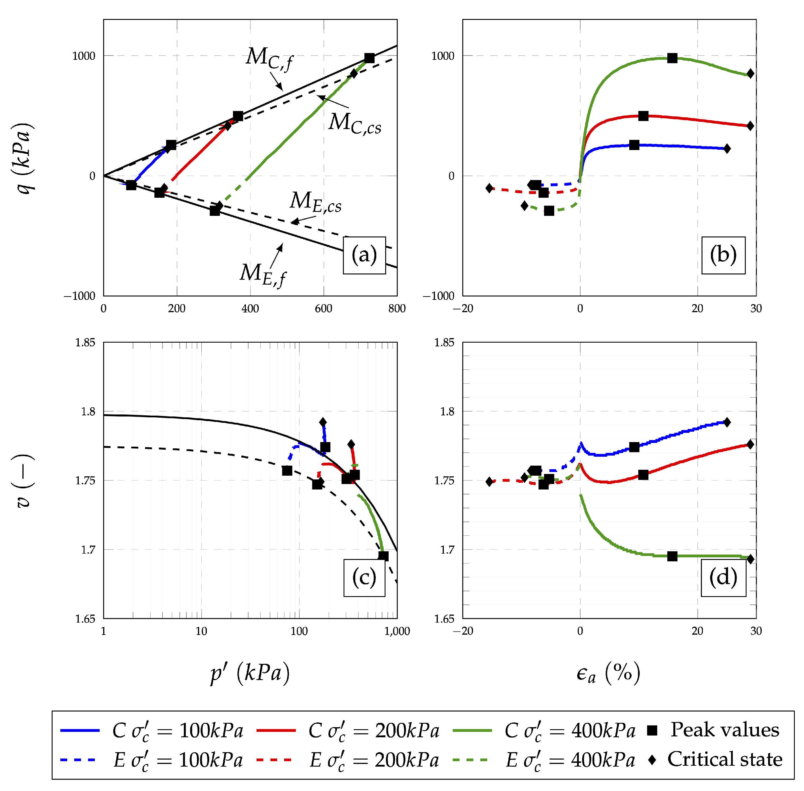
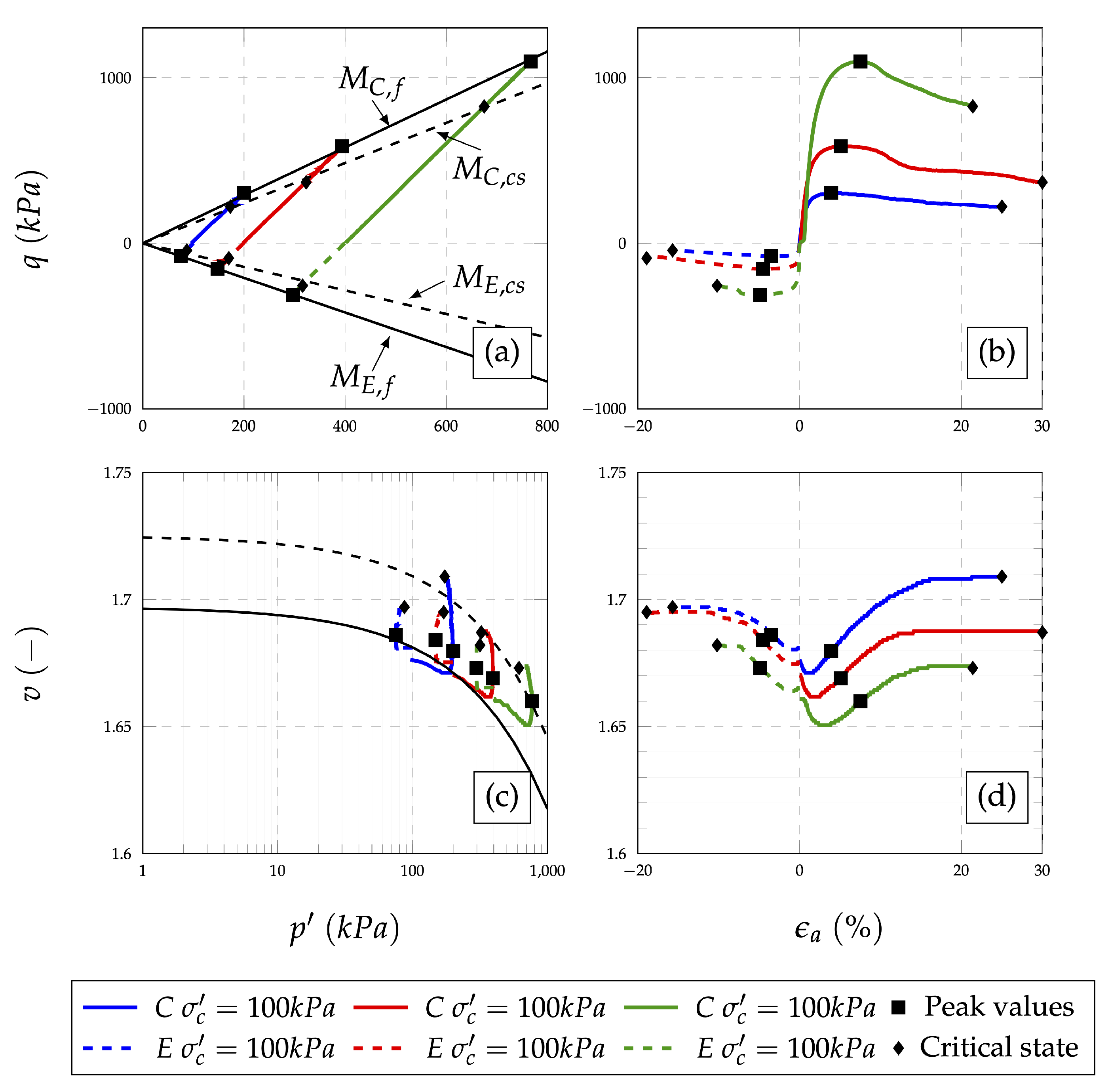
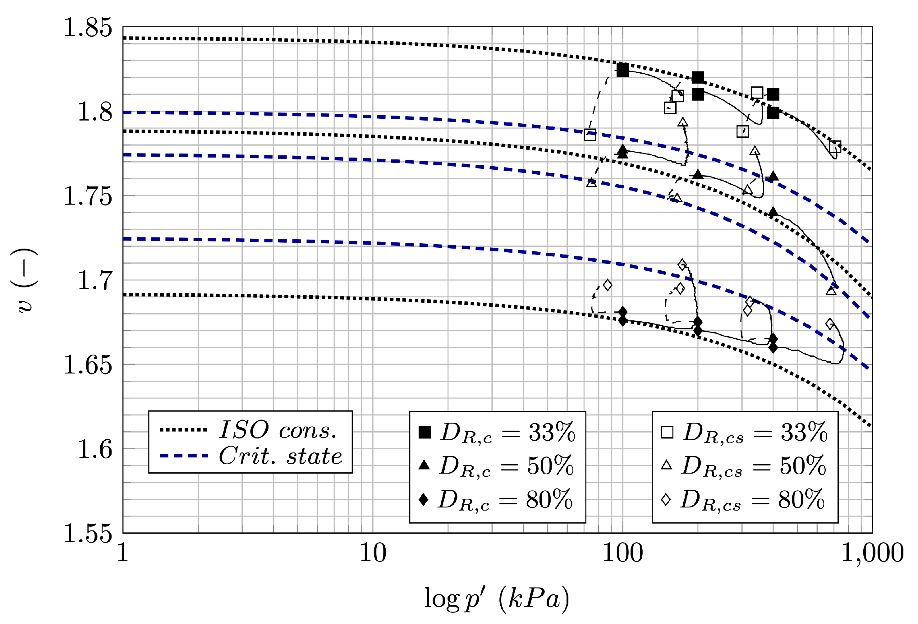
• samples prepared at lower initial density ($D_R=33\%$) show delicate behaviour and the influence of initial density on shear behaviour;
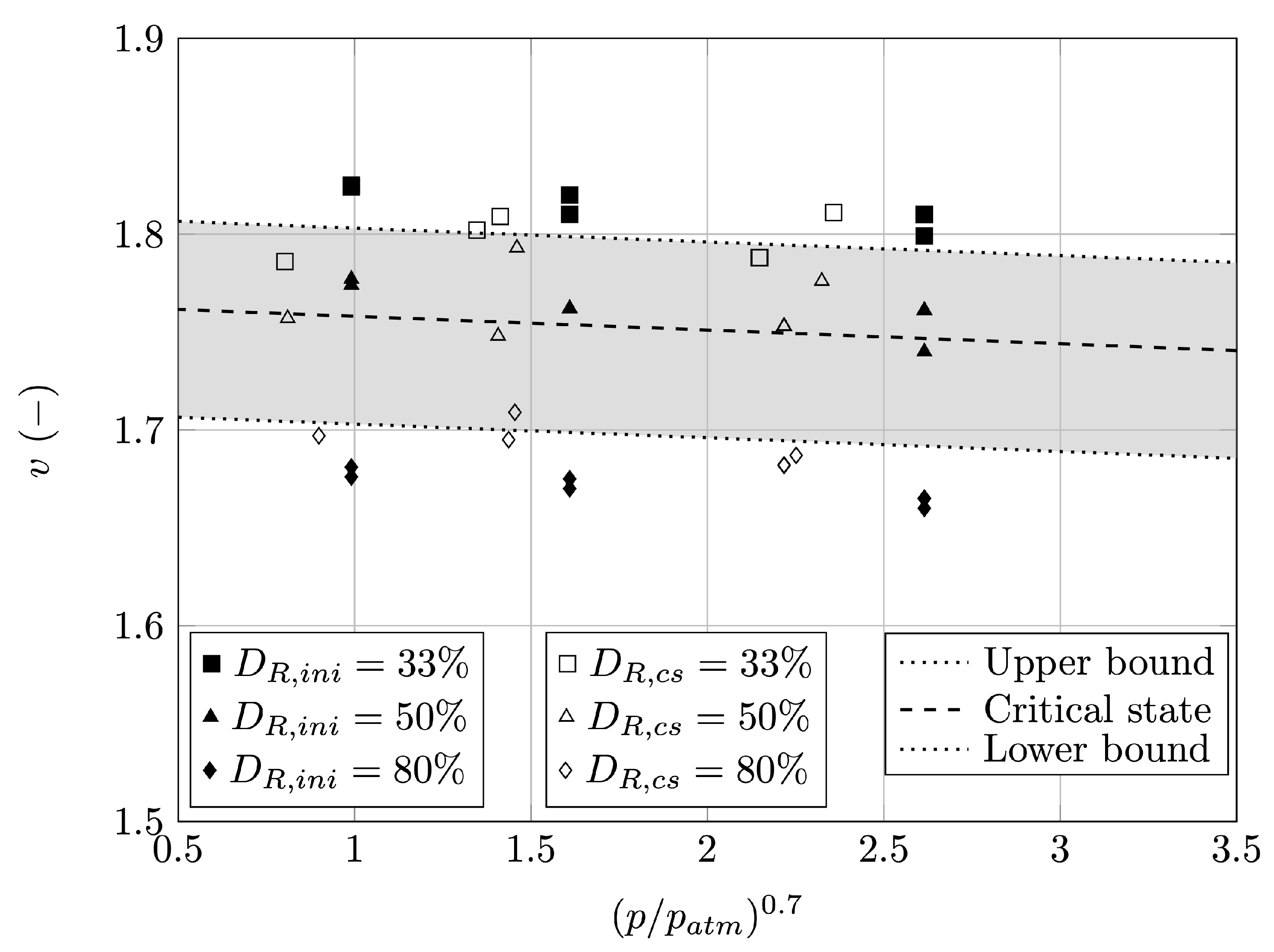
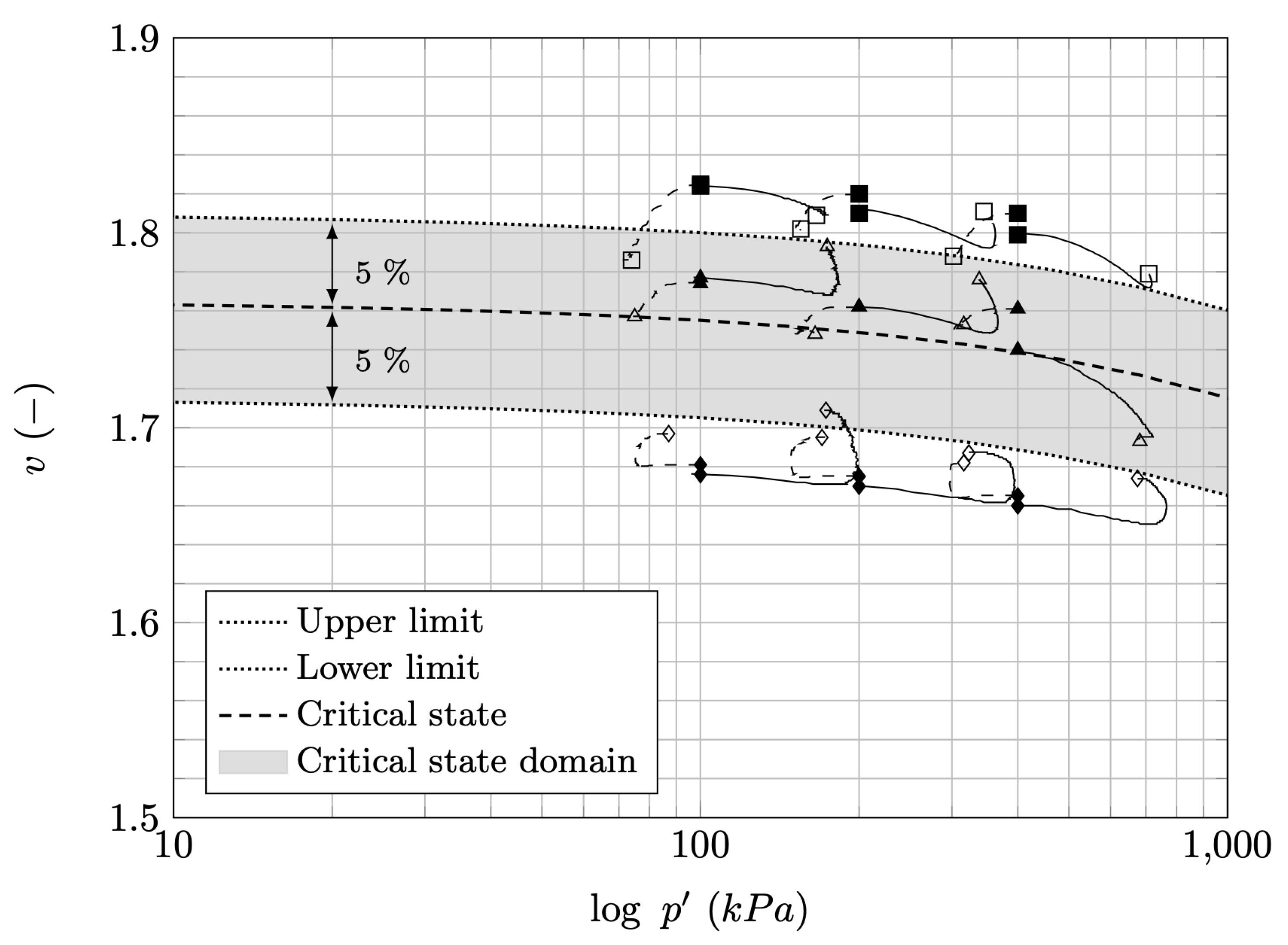
• based on $v-p^{\prime }$ and $v-{ϵ}_a$ plots, and the critical specific volume plot, it can be concluded that the density of 57% is the relative density of critical state. This is one of the reasons why the samples prepared at the initial density of 50% show high sensitivity to sample preparation;
• The difference in critical state for compression and extension is noticeable;
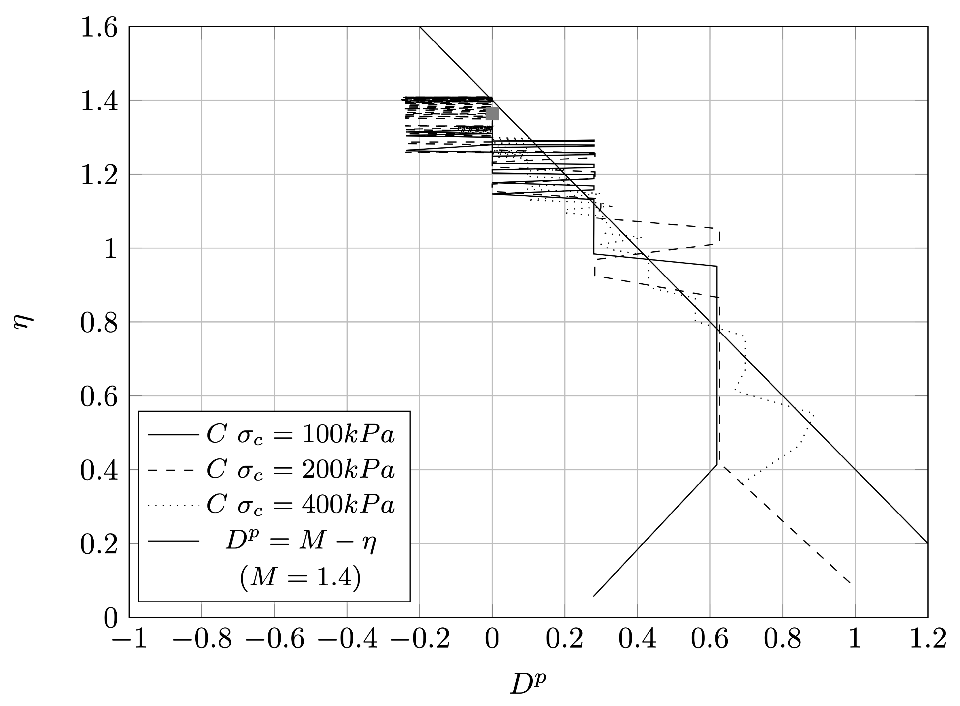
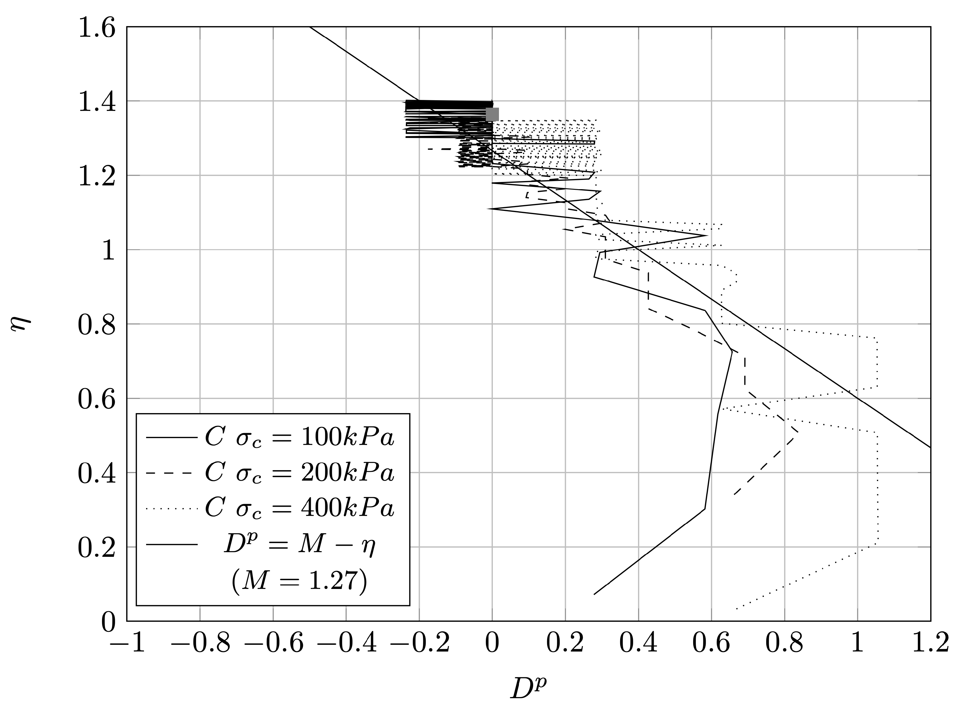
• The value of critical state parameter M is 1.364 which results the critical friction angle of ${\varphi }_{cs}={33.75}^{\circ }$.

References

1. Alarcon-Guzman, A.; Leonards, G.A.; Chameau, J.L. Undrained monotonic and cyclic strength of sands. J. Geotech. Eng. 1988, 114, 1089–1109. [Google Scholar] [CrossRef]
2. Casagrande, A. Liquefaction and cyclic mobility of sands: A critical review. Harv. Soil Mech. Ser. 1976, 88, 1–26. [Google Scholar]
3. Lade, P.V. Static instability and liquefaction of loose fine sandy slopes. J. Geotech. Eng. 1992, 118, 51–71. [Google Scholar] [CrossRef]
4. Roscoe, K.H.; Schofield, A.N.; Wroth, C.P. On the yielding of soils. Géotechnique 1958, 8, 22–53. [Google Scholar] [CrossRef]
5. Schofield, A.N.; Wroth, P. Critical State Soil Mechanics; McGraw-Hill: New York, NY, USA, 1968. [Google Scholar]
6. Wood, D. Soil Behaviour and Critical State Soil Mechanics; Cambridge University Press: Cambridge, UK, 1990. [Google Scholar]
7. Yamamuro, J.A.; Lade, P.V. Static liquefaction of very loose sands. Can. Geotech. J. 1997, 34, 905–917. [Google Scholar] [CrossRef]
8. Bond, A.; Harris, A. Decoding Eurocode 7; CRC Press: London, UK, 2006. [Google Scholar]
9. Been, K.; Jefferies, M.G.; Hachey, J. The critical state of sands. Géotechnique 1991, 41, 365–381. [Google Scholar] [CrossRef]
10. Ishihara, K.; Koga, Y. Case studies of liquefaction in the 1964 Niigata earthquake. Soils Found. 1981, 21, 35–52. [Google Scholar] [CrossRef] [Green Version]
11. Seed, H.B.; Idriss, I.M. Analysis of soil liquefaction: Niigata earthquake. J. Soil Mech. Found. Div. 1967, 93, 83–108. [Google Scholar]
12. Builes, M.; García, E.; Riveros, C.A. Dynamic and static measurements of small strain moduli of toyoura sand. Rev. Fac. Ing. Univ. Antioq. 2008, 43, 86–101. [Google Scholar]
13. Dong, Q.; Xu, C.; Cai, Y.; Juang, H.; Wang, J.; Yang, Z.; Gu, C. Drained instability in loose granular material. Int. J. Geomech. 2016, 16. [Google Scholar] [CrossRef]
14. Le, B.N.; Toyota, H.; Takada, S. Detection of Elastic Region Varied by Inherent Anisotropy of Reconstituted Toyoura Sand; Springer: Berlin/Heidelberg, Germany, 2018; pp. 76–89. [Google Scholar] [CrossRef]
15. Oda, M.; Koishikawa, I.; Higuchi, T. Experimental study of anisotropic shear strength of sand by plane strain test. Soils Found. 1978, 18, 25–38. [Google Scholar] [CrossRef] [Green Version]
16. Verdugo, R.; Ishihara, K. The steady state of sandy soils. Soils Found. 1996, 36, 81–91. [Google Scholar] [CrossRef] [Green Version]
17. Yang, Z.X.; Li, X.S.; Yang, J. Undrained anisotropy and rotational shear in granular soil. Geotechnique 2007, 57, 371–384. [Google Scholar] [CrossRef] [Green Version]
18. Youn, J.U.; Choo, Y.W.; Kim, D.S. Measurement of small-strain shear modulus Gmax of dry and saturated sands by bender element, resonant column, and torsional shear tests. Can. Geotech. J. 2008, 45, 1426–1438. [Google Scholar] [CrossRef]
19. Lade, P.V.; Liggio, C.D.; Yamamuro, J.A. Effects of non-plastic fines on minimum and maximum void ratios of sand. Geotech. Test. J. 1998, 21, 336–347. [Google Scholar] [CrossRef]
20. Won, M.S.; Ling, H.I.; Kim, Y.S. A study of the deformation of flexible pipes buried under model reinforced sand. KSCE J. Civ. Eng. 2004, 8, 377–385. [Google Scholar] [CrossRef]
21. Bastidas, A.M.P.; Boulanger, R.W.; Carey, T.; DeJong, J. Ottawa F-65 Sand Data from Ana Maria Parra Bastidas, NEEShub. 2016. Available online: https://datacenterhub.org/resources/14288 (accessed on 8 May 2020).
22. Yang, L.; Salvati, L. Small strain properties of sands with different cement types. In Proceedings of the International Conferences on Recent Advances in Geotechnical Earthquake Engineering and Soil Dynamics 2010, San Diego, CA, USA, 26 May 2010. [Google Scholar]
23. Zhang, H. Steady State Behaviour of Sands and Limitations of the Triaxial Test. Ph.D. Thesis, University of Ottawa, Ottawa, ON, Canada, 1997. [Google Scholar]
24. Chang, N.; Hseih, N.; Samuelson, D.; Horita, M. Static and cyclic behaviour of monterey# 0 sand. In Proceedings of the 3rd Microzonation Conference, Seattle, WA, USA, 28 June–1 July 1981; pp. 929–944. [Google Scholar]
25. Mulilis, J.P.; Horz, R.C.; Townsend, F.C. The Effects of Cyclic Triaxial Testing Techniques on the Liquefaction Behavior of Monterey No. 0 Sand; US Department of Defense, Department of the Army, Corps of Engineers: Washington, DC, USA, 1976.
26. Saxena, S.K.; Reddy, K.R. Dynamic moduli and damping ratios for Monterey No.0 sand by resonant column tests. Soils Found. 1989, 29, 37–51. [Google Scholar] [CrossRef] [Green Version]
27. Been, K.; Jefferies, M.G. A state parameter for sands. Géotechnique 1985, 35, 99–112. [Google Scholar] [CrossRef]
28. Been, K.; Jefferies, M. Stressdilatancy in very loose sand. Can. Geotech. J. 2004, 41, 972–989. [Google Scholar] [CrossRef]
29. Kang, X.; Xia, Z.; Chen, R.; Ge, L.; Liu, X. The critical state and steady state of sand: A literature review. Mar. Georesour. Geotechnol. 2019, 37, 1105–1118. [Google Scholar] [CrossRef]
30. Malvić, T.; Velić, J. Neogene tectonics in croatian part of the pannonian basin and reflectance in hydrocarbon accumulations. In New Frontiers in Tectonic Research; Schattner, U., Ed.; IntechOpen: Rijeka, Croatia, 2011; Chapter 8. [Google Scholar] [CrossRef] [Green Version]
31. Bošnjak, J. Construction of roads with sand. In Road Management in Republic of Croatia; Sršen, M., Ed.; Croatian Road Society Via-Vita: Zagreb, Croatia, 1995; pp. 536–543. (In Croatian) [Google Scholar]
32. Dimter, S.; Babić, B. Stabilizing effect of fly ash on the Drava sand. Gradevinar 1997, 49, 685–693. [Google Scholar]
33. Dimter, S.; Rukavina, T.; Dragčević, V. Strength properties of fly ash stabilized mixes. Road Mater. Pavement Des. 2011, 12, 687–697. [Google Scholar] [CrossRef]
34. Magaš, N. Basic Geological Map of SFRY 1:100,000, Osijek Sheet L34-86); Geološki Zavod Zagreb, Savezni Geološki Zavod: Beograd, Serbia, 1987. (In Croatian) [Google Scholar]
35. Kavre Piltaver, I.; Peter, R.; Šarić, I.; Salamon, K.; Jelovica Badovinac, I.; Koshmak, K.; Nannarone, S.; Delač Marion, I.; Petravić, M. Controlling the grain size of polycrystalline TiO2 films grown by atomic layer deposition. Appl. Surf. Sci. 2017, 419, 564–572. [Google Scholar] [CrossRef]
36. Šarić, I.; Peter, R.; Markovic, M.K.; Badovinac, I.J.; Rogero, C.; Ilyn, M.; Knez, M.; Ambrožić, G. Introducing the concept of pulsed vapor phase copper-free surface click-chemistry using the ALD technique. Chem. Commun. 2019, 55, 3109–3112. [Google Scholar] [CrossRef] [PubMed]
37. Mitchell, J.K.; Soga, K. Fundamentals of Soil Behavior; John Wiley & Sons: Hoboken, NJ, USA, 2005; p. 577. [Google Scholar]
38. ISO 17892-3:2015. Geotechnical Investigation and Testing—Laboratory Testing of Soil—Part 3: Determination of Particle Density; Technical Report; ISO: Geneva, Switzerland, 2015. [Google Scholar]
39. ISO 17892-3:2016. Geotechnical Investigation and Testing—Laboratory Testing of Soil—Part 4: Determination of Particle Size Distribution; Technical Report; ISO: Geneva, Switzerland, 2016. [Google Scholar]
40. ASTM D4254-16. Standard Test Methods for Minimum Index Density and Unit Weight of Soils and Calculation of Relative Density; ASTM International: West Conshohocken, PA, USA, 2016. [Google Scholar]
41. ASTM D4253-16. Test Methods for Maximum Index Density and Unit Weight of Soils Using a Vibratory Table; ASTM International: West Conshohocken, PA, USA, 2016. [Google Scholar]
42. Holtz, R.D.; Kovacs, W.D.; Sheahan, T.C. An Introduction to Geotechnical Engineering; Pearson: London, UK, 2011. [Google Scholar]
43. Smith, I. Smith’s Elements of Soil Mechanics; Wiley: Hoboken, NJ, USA, 2014. [Google Scholar]
44. Controls. Automatic Triaxial Tests System—AUTOTRIAX 2, Soil Mechanics Testing Equipment; Controls: Liscate MI, Italy, 2020. [Google Scholar]
45. ASTM. Method for Consolidated Drained Triaxial Compression Test for Soils; ASTM: West Conshohocken, PA, USA, 2011. [Google Scholar] [CrossRef]
46. Lade, P.V. Triaxial Testing of Soils; Wiley: Hoboken, NJ, USA, 2016. [Google Scholar]
47. Panda, R.C. Introduction to PID Controllers: Theory, Tuning and Application to Frontier Areas; OCLC: 908265492; InTech: Rijeka, Croatia, 2012. [Google Scholar]
48. Omar, T.; Sadrekarimi, A. Specimen size effects on behavior of loose sand in triaxial compression tests. Can. Geotech. J. 2015, 52, 732–746. [Google Scholar] [CrossRef]
49. Ladd, R. Preparing test specimens using under compaction. Geotech. Test. J. 1978, 1, 16–23. [Google Scholar] [CrossRef]
50. Oda, M. Initial fabrics and their relations to mechanical properties of granular material. Soils Found. 1972, 12, 17–36. [Google Scholar] [CrossRef] [Green Version]
51. Frost, J.; Park, J.Y. A critical assessment of the moist tamping technique. Geotech. Test. J. 2003, 26, 57–70. [Google Scholar] [CrossRef]
52. Murthy, T.G.; Loukidis, D.; Carraro, J.A.H.; Prezzi, M.; Salgado, R. Undrained monotonic response of clean and silty sands. Géotechnique 2007, 57, 273–288. [Google Scholar] [CrossRef]
53. Vucetic, M.; Dobry, R. Cyclic triaxial strain-controlled testing of liquefiable sands. In Advanced Triaxial Testing of Soil and Rock; ASTM International: West Conshohocken, PA, USA, 1988; pp. 475–485. [Google Scholar] [CrossRef]
54. Ratkowsky, D. Handbook of Nonlinear Regression Models; Statistics, Textbooks and Monographs; M. Dekker: New York, NY, USA, 1990. [Google Scholar]
55. Seber, G.; Wild, C. Nonlinear Regression; Wiley Series in Probability and Statistics; Wiley: Hoboken, NJ, USA, 2005. [Google Scholar]
56. Massaron, L.; Boschetti, A. Regression Analysis with Python; Packt Publishing: Birmingham, UK, 2016. [Google Scholar]
57. Yang, J.; Luo, X. Exploring the relationship between critical state and particle shape for granular materials. J. Mech. Phys. Solids 2015, 84, 196–213. [Google Scholar] [CrossRef]
58. Azeiteiro, R.J.N.; Coelho, P.A.L.F.; Taborda, D.M.G.; Grazina, J.C.D. Critical state–based interpretation of the monotonic behavior of hostun sand. J. Geotech. Geoenviron. Eng. 2017, 143, 04017004. [Google Scholar] [CrossRef]
59. Loukidis, D.; Salgado, R. Modeling sand response using two-surface plasticity. Comput. Geotech. 2009, 36, 166–186. [Google Scholar] [CrossRef]
60. Vaid, Y.; Sasitharan, S. The strength and dilatancy of sand. Can. Geotech. J. 1992, 29, 522–526. [Google Scholar] [CrossRef]
61. Nova, R.; Wood, D. A constitutive model for soil under monotonic and cyclic loading. In Soil Mechanics-Transient and Cyclic Loading; Wiley: New York, NY, USA, 1982; pp. 343–373. [Google Scholar]
62. Jefferies, M.G.; Shuttle, D.A. Dilatancy in general Cambridge-type models. Géotechnique 2002, 52, 625–638. [Google Scholar] [CrossRef]
63. Szypcio, Z. Stress-dilatancy for soils. Part II: Experimental validation for triaxial tests. Studia Geotech. Mech. 2016, 38, 59–65. [Google Scholar] [CrossRef] [Green Version]
64. Jefferies, M.; Been, K. Soil Liquefaction; CRC Press: London, UK, 2015. [Google Scholar] [CrossRef]
65. Cornforth, D.H. Plane Strain Failure Characteristics of Saturated Sand. Ph.D. Thesis, Imperial College London, London, UK, 1961. [Google Scholar]
Figure 1. SEM image of the Drava River sand.
Applsci 10 05733 g001
Figure 2. Sieve analysis of DrOS018 sand compared to the similar sand types in literature: Toyoura sand: T1—[14], T2—[13], T3—[18], T4—[12]; Ottawa sand: O1—[12], O2—[22], O3—[23], O4—[7]; Nevada sand: N1—[20], N2—[19], N3—[7]; Monterey sand: M1—[22], M2—[25].
Applsci 10 05733 g002
Figure 3. Scheme of static triaxial system: (a) triaxial cell, (b) sample, (c) load cell, (d) Linear Variable Differential Transformer, (e) cell pressure transducer, (f) pore water pressure transducer, (g) back pressure transducer, (h) volume controller, (i) pneumatic pressure system, (j) deaired water tank, (k) servo-flow, (l) RTC module, (m) ATD data logger, (n) personal computer, (o) compressed air distributor.
Applsci 10 05733 g003
Figure 4. Triaxial sample: (a) sample preparation using undercompaction method and (b) prepared sample.
Applsci 10 05733 g004
Figure 5. Triaxial test results on sample with relative density 33%: (a) mean stress p vs. deviatoric stress q, (b) axial strain ϵ a vs. deviatoric stress q, (c) mean stress p vs. specific volume v and (d) axial strain ϵ a vs. specific volume v.
Applsci 10 05733 g005
Figure 6. Triaxial test results on sample with relative density 50 % : (a) mean stress p vs. deviatoric stress q, (b) axial strain ϵ a vs. deviatoric stress q, (c) mean stress p vs. specific volume v and (d) axial strain ϵ a vs. specific volume v.
Applsci 10 05733 g006
Figure 7. Triaxial test results on sample with relative density 80 % : (a) mean stress p vs. deviatoric stress q, (b) axial strain ϵ a vs. deviatoric stress q, (c) mean stress p vs. specific volume v and (d) axial strain ϵ a vs. specific volume v.
Applsci 10 05733 g007
Figure 8. Critical state of DrOS018 sand.
Applsci 10 05733 g008
Figure 9. Volumetric behaviour in normalised mean effective plane.
Applsci 10 05733 g009
Figure 10. Critical state of DrOS018 sand with upper and lower bound curves.
Applsci 10 05733 g010
Figure 11. Plastic dilatancy for relative density D r = 33 % .
Applsci 10 05733 g011
Figure 12. Plastic dilatancy for relative density D r = 50 % .
Applsci 10 05733 g012
Figure 13. Plastic dilatancy for relative density D r = 80 % .
Applsci 10 05733 g013
Figure 14. Plastic dilatancy versus maximum stress ratio (* according to [60,62,65]).
Applsci 10 05733 g014
Figure 15. Variation of friction angle with state parameter (* according to [64]).
Applsci 10 05733 g015
Figure 16. Volumetric strain at peak friction angle for drained triaxial tests (* according to [64]).
Applsci 10 05733 g016