Article

State-Constrained Sub-Optimal Tracking Controller for Continuous-Time Linear Time-Invariant (CT-LTI) Systems and Its Application for DC Motor Servo Systems

1
Department of Electrical and Biomedical Engineering, Hanyang University, Seoul 04763, Korea
2
Department of Electrical Engineering, Hanyang University, Seoul 04763, Korea
*
Authors to whom correspondence should be addressed.
Appl. Sci. 2020, 10(16), 5724; https://doi.org/10.3390/app10165724
Submission received: 22 July 2020 / Revised: 10 August 2020 / Accepted: 13 August 2020 / Published: 18 August 2020
(This article belongs to the Special Issue New Trends in the Control of Robots and Mechatronic Systems)

Abstract

:
In this paper, we propose an analytic solution of state-constrained optimal tracking control problems for continuous-time linear time-invariant (CT-LTI) systems that are based on model-based prediction, the quadratic penalty function, and the variational approach. Model-based prediction is a concept taken from model-predictive control (MPC) and this is essential to change the direction of calculation for the solution from backward to forward. The quadratic penalty function plays an important role in deriving the analytic solution since it can transform the problem into a form that does not have inequality constraints. For computational convenience, we also propose a sub-optimal controller derived from the steady-state approximation of the analytic solution and show that the proposed controller satisfies the Lyapunov stability. The main advantage of the proposed controller is that it can be implemented in real time with a lower computational load compared to the implicit MPC. Finally, the simulation results for a DC motor servo system are shown and compared with the results of the direct multi-shooting method and the implicit MPC to verify the effectiveness of the proposed controller.

Graphical Abstract

1. Introduction

Recently, interest has been increasing in control systems that require limitations on the state of the target system. For example, optimal trajectory control for industrial robots [1,2], which limits the workspace for co-work between humans and machines, and optimal powertrain control for hybrid vehicle systems [3,4,5], which has limitations on battery capacity, have become more critical to industry. For analytical and computational convenience, the target system for industrial purposes is often linearized, therefore several studies on linear optimal controllers with state constraints were performed. However, these studies imply large computational loads that make it difficult to implement in real time. The following section explains why these computational loads are caused.

1.1. Solutions and Their Approximations of the Optimal Control Problems

Assume that the target system is a continuous-time linear time-invariant (CT-LTI) system as follows:
x ˙ = A x + B u ,
y = C y x ,
where x ( t ) is the state of the system, u ( t ) is the input of the system, and y ( t ) is the output of the system. Let the tracking error e ( t ) be
e = r y ,
where r ( t ) is the reference for the output. Then, the linear-quadratic tracking (LQT) problem can be expressed as follows [6,7,8]:
minimize   e , u J = 1 2 t 0 t f ( e T Q e + u T R u ) d t subject   to   A x + B u x ˙ = 0 ,
where Q and R are positive definite matrices weighting for the tracking error and the input, J is the cost function, t 0 is the initial time, and t f is the final time. Assume that pair ( A , B ) is controllable and pair ( A , C y ) is observable. Then, by the Lagrange multiplier method [6,7,8] and the variational approach (Theorem A1), the LQT problem (4) can be transformed into a problem of finding solutions of the Riccati equation with boundary conditions and an auxiliary dynamic equation related to the reference. The Riccati equation and the auxiliary dynamic equation can be derived as follows:
P ˙ = P A A T P + P B R 1 B T P C y T Q C y ,
g ˙ = ( A T P B R 1 B T ) g C y T Q r ,
where P ( t ) and g ( t ) are the solutions to be determined. These solutions are usually calculated in the backward direction in time or by using iterations since A B R 1 B T P , which is the system matrix of the closed-loop system, must have all the negative real parts of the eigenvalues. However, if there are no constraints on the input and the state, it is well known in control engineering that the solutions of the equations can be approximated to their steady-state values, and the solutions become independent of the time. In the case of input constraints alone, the optimal input can be determined by Pontryagin’s minimum principle [6,7,8,9]. In general, the solutions determined by Pontryagin’s minimum principle are closely related with the solutions of the Equations (5) and (6) and have a form simple enough to be implemented on modern microcontrollers. On the other hand, if there are inequality constraints on the state, the problem statement (4) is not valid, therefore it must be redefined as follows:
minimize   e , u J = 1 2 t 0 t f ( e T Q e + u T R u ) d t subject   to     { A x + B u x ˙ = 0 C h x + w 0   ,
where C h and w are time-invariant parameters of the inequality constraints. The vector inequality h 0 means that h i 0   ( i = 1 , , n ) , where h = [ h 1 h n ] T . In this case, the problem related to the direction of the calculation is hard to avoid.
Since the problem (7) is difficult to solve exactly, many kinds of research were proposed to solve this problem approximately. The first group of research consists of numerical approaches including dynamic programming methods [6,10,11] or direct and indirect methods [11,12,13]. In general, these methods discretize the target system and apply numerical methods. Since this procedure does not change the direction of the calculation, most of these methods need backward calculations or iterations for all the time steps. The second group of research comprises model-predictive control (MPC) methods including implicit MPC [14,15,16,17] and explicit MPC [18,19,20]. The main difference from the first group is that time-forward calculation is possible since this method predicts the optimal states and inputs of the target system for a short time ahead. However, this method also requires repetitive calculations for the predictions, and the precision of the calculation decreases if the time length of the prediction is not long enough, therefore it still requires many computations in general. To reduce the computational load, explicit MPC was proposed. For explicit MPC design, methods dividing the state space are essential, but the results of these methods are not easy to analyze in practice [21] since they are based on numerical iterations. In summary, the computational problem of the state-constrained optimal tracking control is that the direction of the exact computation for the solution is a time-backward calculation which leads to increasing computational loads.

1.2. Outline and Scope of the Paper

In this paper, we propose an analytic solution of state-constrained optimal tracking control problems for CT-LTI systems that are based on the model-based prediction, the quadratic penalty method, and the variational approach in Section 2. The model-based prediction is a concept taken from MPC, and this is essential to change the direction of the calculation for the solution from backward to forward. The quadratic penalty method plays an important role in deriving the analytic solution since it can transform the problem into a form that does not have inequality constraints. For computational convenience, we also propose a sub-optimal controller derived from the steady-state approximation of the analytic solution, and show that the proposed controller satisfies the Lyapunov stability in Section 3. Finally, the simulation results for a DC motor servo system are shown and compared with the results of the direct multi-shooting method and implicit MPC to verify the effectiveness of the proposed controller in Section 4.

2. Analytic Solution of State-Constrained Optimal Tracking Problems

In this section, we describe the analytic solution of state-constrained optimal tracking problems. This solution can be derived by using the model-based prediction, inequality constraints using prediction, the quadratic penalty function, and the variational approach.

2.1. Model-Based Prediction

Suppose that the target system is equal to (1), then a model-based prediction with a fixed time interval τ can be written as follows [16,22]:
x ^ τ ( t ) = x ( t + τ | t ) = e A τ x ( t ) + t t + τ e A ( t + τ η ) B u ( η ) d η
Assume that the time interval τ is short enough to consider the input as a constant. Then, we can approximate (8) as
x ^ τ A d x + B d u ,
where
A d ( τ ) = e A τ   and   B d ( τ ) = 0 τ e A η d η   B .
The calculation of the above matrices is described in [22] (pp. 114–117) and this can be performed by using c2d MATLAB® command, etc.

2.2. Inequality Constraints Using Prediction

Assume that the left sides of the inequality constraints are
h i ( x ) = C h _ i x + w i ,   ( i = 1 , 2 , , n ) ,
where
C h = [ C h _ 1 C h _ n ]   and   w = [ w 1 w n ] .
Then, the inequality constraints have a form of
h i ( x ) 0
Since (11) should be valid at all times, the following inequalities also should be valid:
h i ( x ^ τ ) 0
Let
h ( x , u ) = [ h 1 ( x ) h n ( x ) h 1 ( x ^ τ ) h n ( x ^ τ ) ] = [ C h x + w C h A d x + C h B d u + w ] ,
where
C h = [ C h _ 1 C h _ 2 C h _ n ] ,   w = [ w 1 w 2 w n ] .
Then, (11) and (12) can be rewritten by using (13) as follows:
h ( x , u ) 0 .

2.3. Quadratic Penalty Function

Suppose that the penalty function p i of the inequality constraint h i 0 is
p i ( h i ) = 1 2 α i ( h i ) h i 2 ,   ( i = 1 , 2 , , 2 n ) ,
where
α i ( h i ) = { 0 ,   h i < 0 q i ,   h i 0   ,
and q i > 0 is the weight for α i [23,24]. As shown in Figure 1, the meaning of the penalty function is the violation costs of the inequality constraint.
The quadratic penalty function is defined as the sum of the penalty functions:
p ( h ) = i = 1 2 n p i ( h i ) = 1 2 h T ( x , u ) diag ( α T )   h ( x , u ) ,
where
α = [ α x α τ ] ,   α x = [ α 1 α n ] ,   and   α τ = [ α n + 1 α 2 n ] ,
and the diag function is defined as
diag ( [ σ 1 σ 2 σ n ] ) = [ σ 1 0 0 0 σ 2 0 0 0 σ n ] .

2.4. Variational Approach

By using the Lagrange multiplier method and the penalty function method [23,24], Problem (7) can be transformed into the following problem:
minimize   x , u J a = t 0 t f L ( x , x ˙ , u ) d t ,
L ( x , x ˙ , u ) = 1 2 ( r C y x ) T Q ( r C y x ) + 1 2 u T R u + λ T ( A x + B u x ˙ ) + 1 2 h T diag ( α T )   h ,
where λ ( t ) is the Lagrange multiplier. Let the Hamiltonian function of (17) be
H ( x , u ) = 1 2 ( r C y x ) T Q ( r C y x ) + 1 2 u T R u + λ T ( A x + B u ) + 1 2 h T diag ( α T )   h ,
and Q x = diag ( α x T ) , Q τ = diag ( α τ T ) . Then, substituting (13) into (19) yields
H ( x , u ) = 1 2 ( r C y x ) T Q ( r C y x ) + 1 2 u T R u + λ T ( A x + B u ) + 1 2 ( C h x + w ) T Q x ( C h x + w ) + 1 2 ( C h A d x + C h B d u + w ) T Q τ ( C h A d x + C h B d u + w ) .
By Corollary A1, the following equations hold:
λ ˙ = C y T Q ( r C y x ) A T λ C h T Q x ( C h x + w ) A d T C h T Q τ ( C h A d x + C h B d u + w ) = A T λ ( Q 1 + A d T C h T Q τ C h A d ) x A d T C h T Q τ C h B d u + C y T Q r ( C h T Q x + A d T C h T Q τ ) w ,
0 = u T R + λ T B + ( C h A d x + C h B d u + w ) T Q τ C h B d ,
Q 1 = C y T Q C y + C h T Q x C h .
Let
R τ = R + B d T C h T Q τ C h B d .
Then, the optimal input is
u = R τ 1 B T λ R τ 1 B d T C h T Q τ C h A d x R τ 1 B d T C h T Q τ w .

2.5. Analytical Solution of the Problem

The following procedure is the same method used in the derivation of the Riccati Equation (5) and the auxiliary dynamic Equation (6) [7,8].
Theorem 1.
Assume that the costate is proportional to the state. Then, the costate can be written as
λ = P x g ,
where P ( t ) and g ( t ) are values to be determined. Then, the following dynamic equations hold:
P ˙ = P A z A z T P + P B R τ 1 B T P Q 2 ,
g ˙ = ( A z T P B R τ 1 B T ) g C y T Q r + [ C h T Q x P B R τ 1 B d T C h T Q τ + A d T C h T Q τ ( I C h B d R τ 1 B d T C h T Q τ ) ] w ,
where
Q 2 = Q 1 + A d T C h T Q τ ( I C h B d R τ 1 B d T C h T Q τ ) C h A d ,
A z = A B R τ 1 B d T C h T Q τ C h A d .
Proof. 
By differentiating (26),
λ ˙ = P ˙ x + P x ˙ g ˙ .
Substituting (1), (25), and (26) into (31) yields
λ ˙ = ( P ˙ + P A ) x + P B u g ˙ = ( P ˙ + P A z ) x P B R τ 1 B T λ P B R τ 1 B d T C h T Q τ w g ˙ = ( P ˙ + P A z P B R τ 1 B T P ) x g ˙ + P B R τ 1 B T g P B R τ 1 B d T C h T Q τ w ,
Since the left sides of (21) and (32) are equal, the right sides of (21) and (32) are also equal. Therefore,
0 = ( P ˙ + P A z P B R τ 1 B T P + Q 1 + A d T C h T Q τ C h A d ) x g ˙ + P B R τ 1 B T g + ( C h T Q x + A d T C h T Q τ P B R τ 1 B d T C h T Q τ ) w C y T Q r + A T λ + A d T C h T Q τ C h B d u .
Substituting (25) and (26) into (33) yields
0 = ( P ˙ + P A z + A z T P P B R τ 1 B T P + Q 2 ) x g ˙ ( A z T P B R τ 1 B T ) g C y T Q r + [ C h T Q x P B R τ 1 B d T C h T Q τ + A d T C h T Q τ ( I C h B d R τ 1 B d T C h T Q τ ) ] w .
Since (34) should be valid for all the states, Equations (27) and (28) hold. □

3. State-Constrained Sub-Optimal Tracking Controller

Exact solutions of (27) and (28) have to be calculated in the backward direction in time, and this is not proper for real-time implementations. Therefore, in this section, we propose a sub-optimal controller that is stable and proper for real-time implementations.

3.1. State-Constrained Sub-Optimal Tracking Controller

The steady-state values of (27) and (28) are
0 = P s A z + A z T P s P s B R τ 1 B T P s + Q 2 ,
g s = ( A c T ) 1 C y T Q r + ( A c T ) 1 [ C h T Q x P s B R τ 1 B d T C h T Q τ + A d T C h T Q τ ( I C h B d R τ 1 B d T C h T Q τ ) ] w ,
where
A c = A z B R τ 1 B T P s .
Substituting (26) into (25) yields
u = ( R τ 1 B T P s + R τ 1 B d T C h T Q τ C h A d ) x + R τ 1 B T g s R τ 1 B d T C h T Q τ w .
Notably, (38) becomes the steady-state LQT controller [7,8] that uses steady-state values of (5) and (6) if Q x and Q τ are null matrices.
The sub-optimal controller is implemented by calculating (35)–(38), but α τ is needed in these calculations. Since α x indicates current violations of the state constraints and α τ indicates possible violations of the state constraints that occur in a moment, α τ can be identified approximately by the following procedure:
  • Identify α x using current state values and calculate Q x = diag ( α x T ) .
  • Calculate (24) and (35) using an algebraic Riccati equation solver with Q τ = 0 .
  • Calculate (36)–(38) using the result of step 2 and applying Q τ = 0 .
  • Calculate (9) using the result of step 3.
  • Identify α τ using the result of step 4.
Since α x has limited values (zero or a fixed value for each element), offline calculation results for lower computational loads can be used in step 2. The sub-optimal controller requires the following procedure in addition to the above procedure.
6.
Calculate Q τ = diag ( α τ T ) using the result of step 5.
7.
Calculate (24) and (35) using an algebraic Riccati equation solver with the result of step 6.
8.
Calculate (36)–(38) using the result of step 7.
Since α τ also has limited values, step 7 can be performed offline. The main advantage of this procedure is that the total computation time of the procedure is limited to a fixed upper boundary. In the case of offline calculations of steps 2 and 7, it is obvious that the total computation load of the proposed controller is lower than that of the implicit MPC.

3.2. Stability of the Proposed Controller

By the matrix inversion lemma [25,26],
I C h B d R τ 1 B d T C h T Q τ = I C h B d ( R + B d T C h T Q τ C h B d ) 1 B d T C h T Q τ = ( I + C h B d R 1 B d T C h T Q τ ) 1 ,
I Q τ C h B d R τ 1 B d T C h T = ( I + Q τ C h B d R 1 B d T C h T ) 1 .
Therefore, the following equations hold:
Q 2 = [ C y C h C h A d ] T [ Q 0 0 0 Q x 0 0 0 Q τ ( I + C h B d R 1 B d T C h T Q τ ) 1 ] [ C y C h C h A d ] ,
Q τ ( I + C h B d R 1 B d T C h T Q τ ) 1 = ( I + Q τ C h B d R 1 B d T C h T ) 1 Q τ .
These equations show that Q 2 is positive semi-definite since Q is positive definite and Q x , Q τ are positive semi-definite or null. Assume that pair ( A c , [ C y C h C h A d ] ) is observable since C y is different from C h in general and suitable A d may be selected by changing τ . Then, Equation (35) can be rewritten as
P s A c + A c T P s = ( P s B R τ 1 B T P s + Q 2 ) .
Substituting (36)–(38) into (1) and applying r = 0 and w = 0 yields
x ˙ = A c x .
Therefore, it is concluded that the closed-loop system is stable by the Lyapunov stability theorem [27,28] if the observability condition is satisfied.

3.3. Model Modification for Input Smoothing

The input generated by the proposed controller may have severe vibration that is not found in numerical solutions. To mitigate this, we propose a modification of the plant model including a low pass filter before the input as shown in Figure 2.
The state equation of the modified plant model is
d d t [ x u ] = [ A B 0 β I ] [ x u ] + [ 0 β I ] u ¯ ,
y = [ C y 0 ] [ x u ] .
Then, the problem (7) should be changed as follows:
minimize   e , u , u ¯ J = 1 2 t 0 t f ( [ e u ] T [ Q 0 0 R ] [ e u ] + u ¯ T R ¯ u ¯ ) d t subject   to     { [ A B 0 β I ] [ x u ] + [ 0 β I ] u ¯ [ x ˙ u ˙ ] = 0 [ C h 0 ] [ x u ] + w 0   ,
where R ¯ is the weight for u ¯ . Since this problem can be solved by using the same methods described in Section 2 and Section 3, we omit a detailed description of the solution.

4. Case Study: Application for DC Motor Servo Systems

In this section, to help readers understand how to apply the proposed controller, we show an application of the proposed controller for DC motor servo systems. For precision control of DC motor servo systems, studies including MPC [29], data-driven [30], fuzzy [31], neural network [32], cascade control [33], and the digital twin-based optimization [34] were introduced recently. However, except for MPC, these studies did not consider the state constraints; therefore, we compare MPC and the proposed controller for performance verification. The parameters of the target motor are shown in Table 1. The target motor is a 24 V DC brushed gear motor and its rated torque is 2.94 Nm.
Then, the state equation of the target system is
x ˙ = [ R m L m K b L m 0 K m J m B m J m 0 0 κ m 0 ] x + [ 1 L m 0 0 ] u [ 384.62 13.85 0 1714.29 33.33 0 0 0.25 0 ] x + [ 153.85 0 0 ] u ,
y = [ 0 0 1 ] x .
where
x = [ x 1 x 2 x 3 ] ,
x 1 is the motor current, x 2 is the angular speed of the motor, and x 3 is the angular position of the motor. Let β = 1000 , then the modified plant model is
d d t [ x u ] = A [ x u ] + B u ¯ ,
y = C y [ x u ] ,
where
A = [ 384.62 13.85 0 153.85 1714.29 33.33 0 0 0 0.25 0 0 0 0 0 1000 ] , B = [ 0 0 0 1000 ] , C y = [ 0 0 1 0 ]
Let τ = 0.001 , then the parameters for the prediction can be calculated as
A d = [ 0.67 0.01 0 0.09 1.41 0.96 0 0.07 0 0 1 0 0 0 0 0.33 ] , B d = [ 0.04 0.04 0 0.67 ]
The optimal tracking problem is
minimize   x , u , u ¯ J = 1 2 t 0 t f ( [ r x 3 u ] T [ 100 0 0 1 ] [ r x 3 u ] + u ¯ 2 ) d t subject   to     { A [ x u ] + B u ¯ [ x ˙ u ˙ ] = 0 C h [ x u ] + w 0 ,
where
C h = [ 1 0 0 0 1 0 0 0 0 1 0 0 0 1 0 0 ] , w = [ 3 3 50 50 ]
In this case, [ C y C h C h A d ] has full rank, therefore the closed-loop system is stable. Available values of P s in the cases of Q τ = 0 are shown in Table 2. The weight for α x is [ 10000 10000 0.001 0.001 ] T and P s was calculated by the MATLAB® care function. Since the weight for α τ is [ 100 100 10 10 ] T and similar calculations can be performed in the cases of Q τ 0 , the proposed controller can be implemented by these results. Figure 3 shows the simulation results with r = π and x ( 0 ) = 0 without changing w . The proposed controller was implemented by using Simulink® blocks and the ode2 (Heun) fixed-step solver was used for the simulation. The step size was set at 10μs for smooth results. To verify the performance of the proposed controller, we also implemented an implicit MPC by using MATLAB® Model Predictive Control ToolboxTM software. A numerical method based on the direct multi-shooting method implemented by using CasADi software [35] was chosen for comparison since it is close to the optimal solution. The sampling time used in both the numerical method and the implicit MPC was set to 100 μs since lower sampling time causes larger computational loads. The prediction and control horizon of the MPC is set to (100, 10).
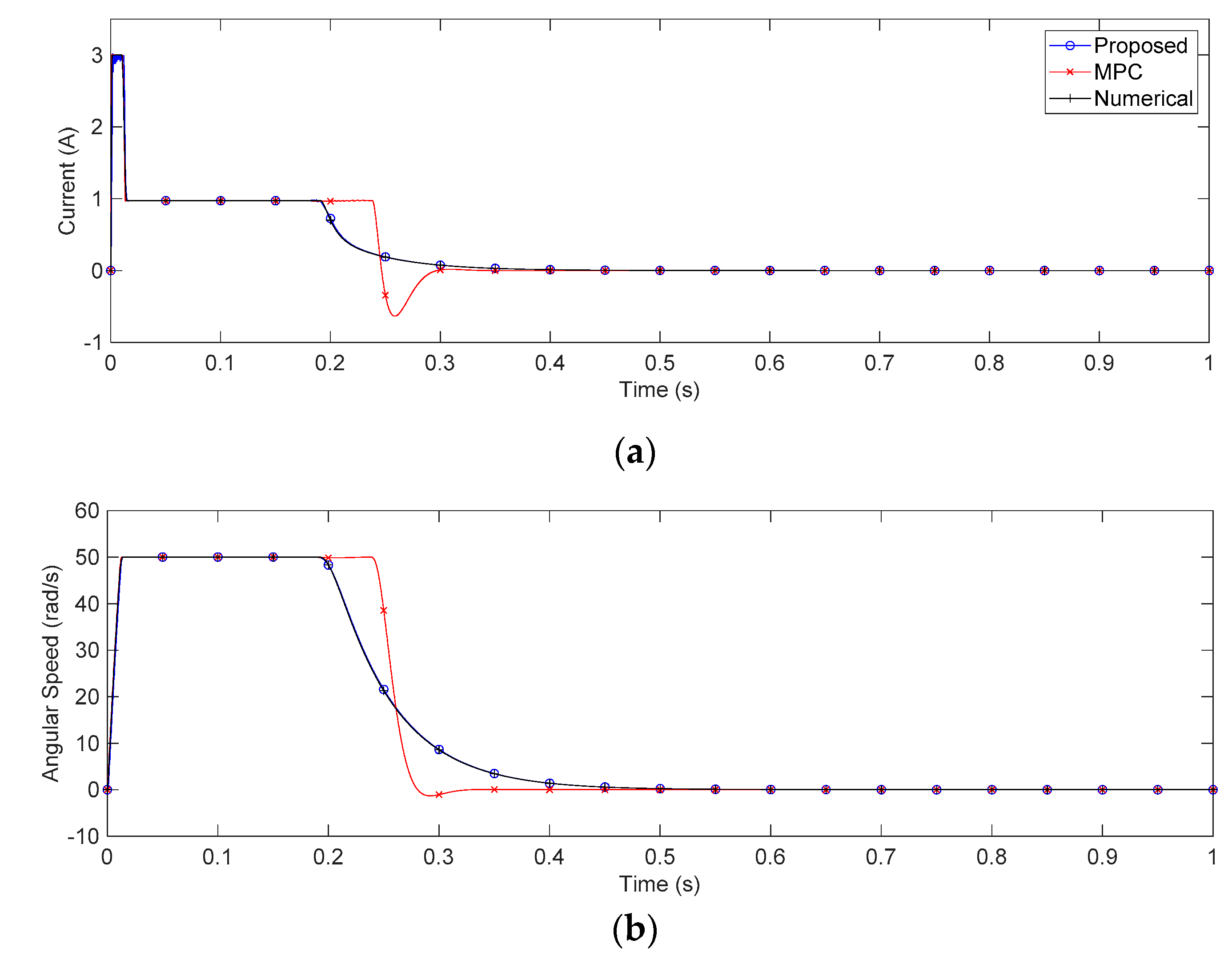
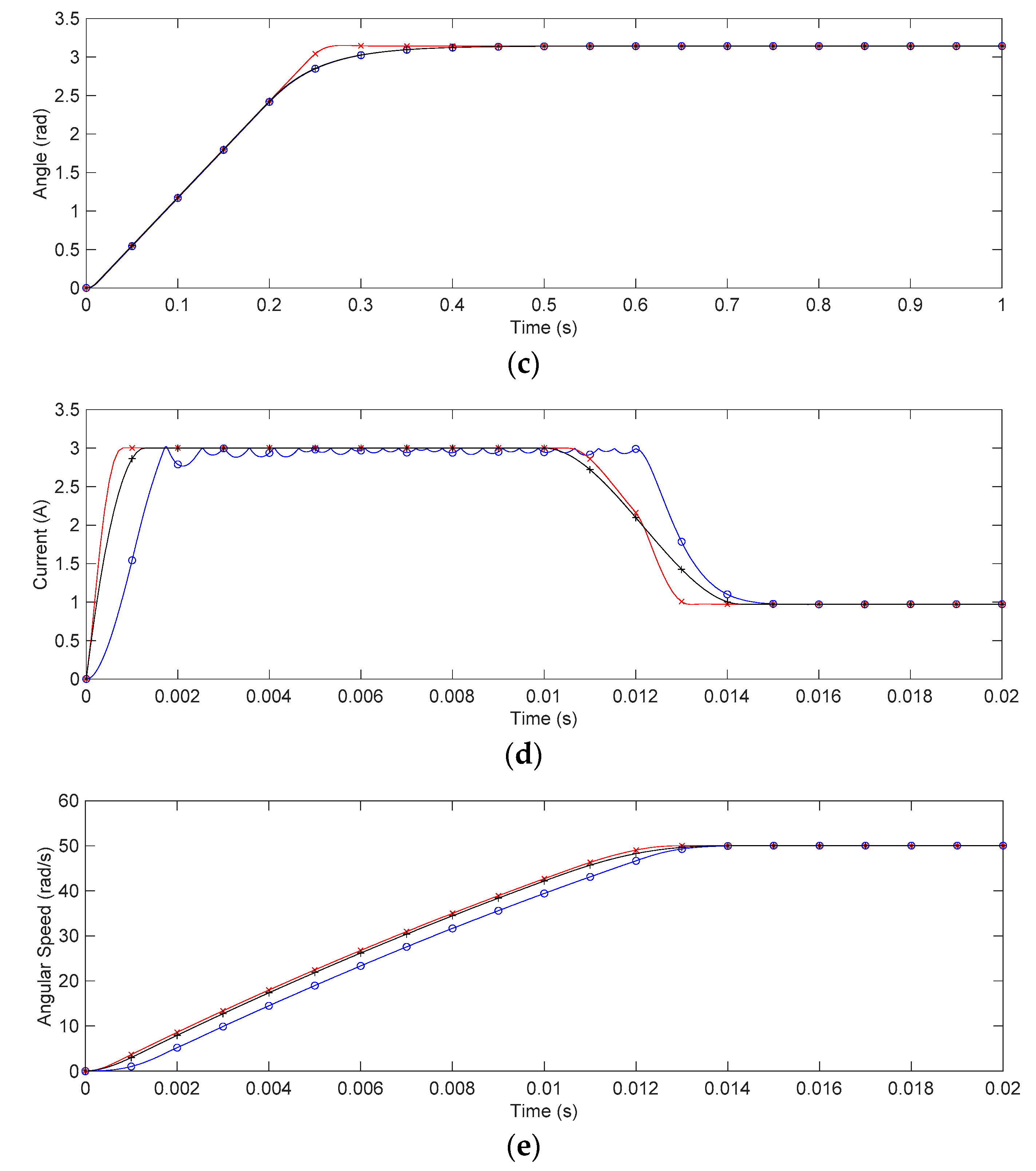
As shown in Figure 3a–c, the trajectory of the proposed controller and that of the numerical method are very similar, therefore it can be said that the proposed controller is well-approximated. On the other hand, the implicit MPC has different trajectories between 0.2 and 0.4 s though the constraints are maintained. In Figure 3d–e, it seems that the trajectory of the proposed controller has a delay compared to that of the numerical method, but the delay is small enough to be neglected. Since the steady-state LQT controller has similar delay properties [36], it is assumed that the cause of this phenomenon is the steady-state approximation.
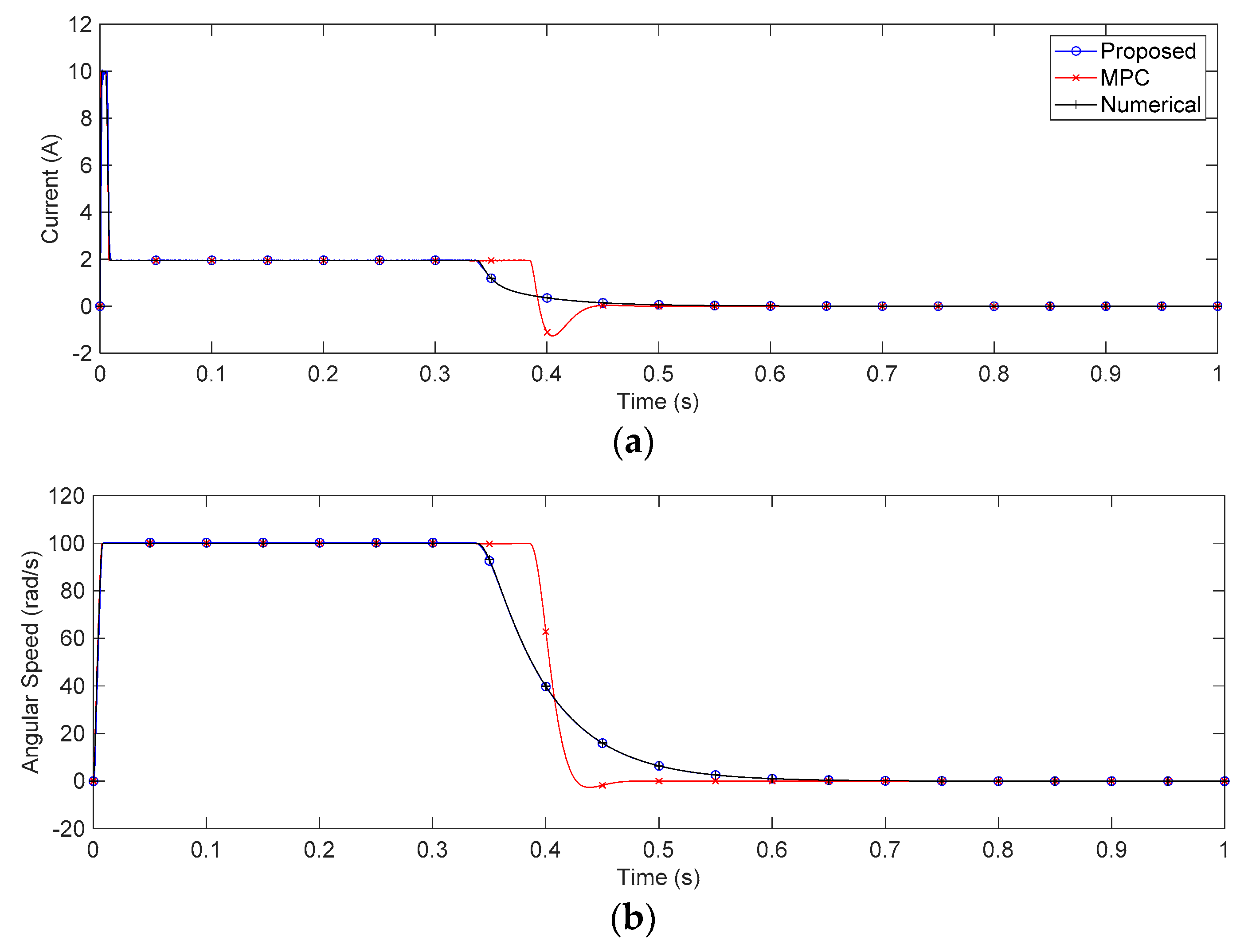
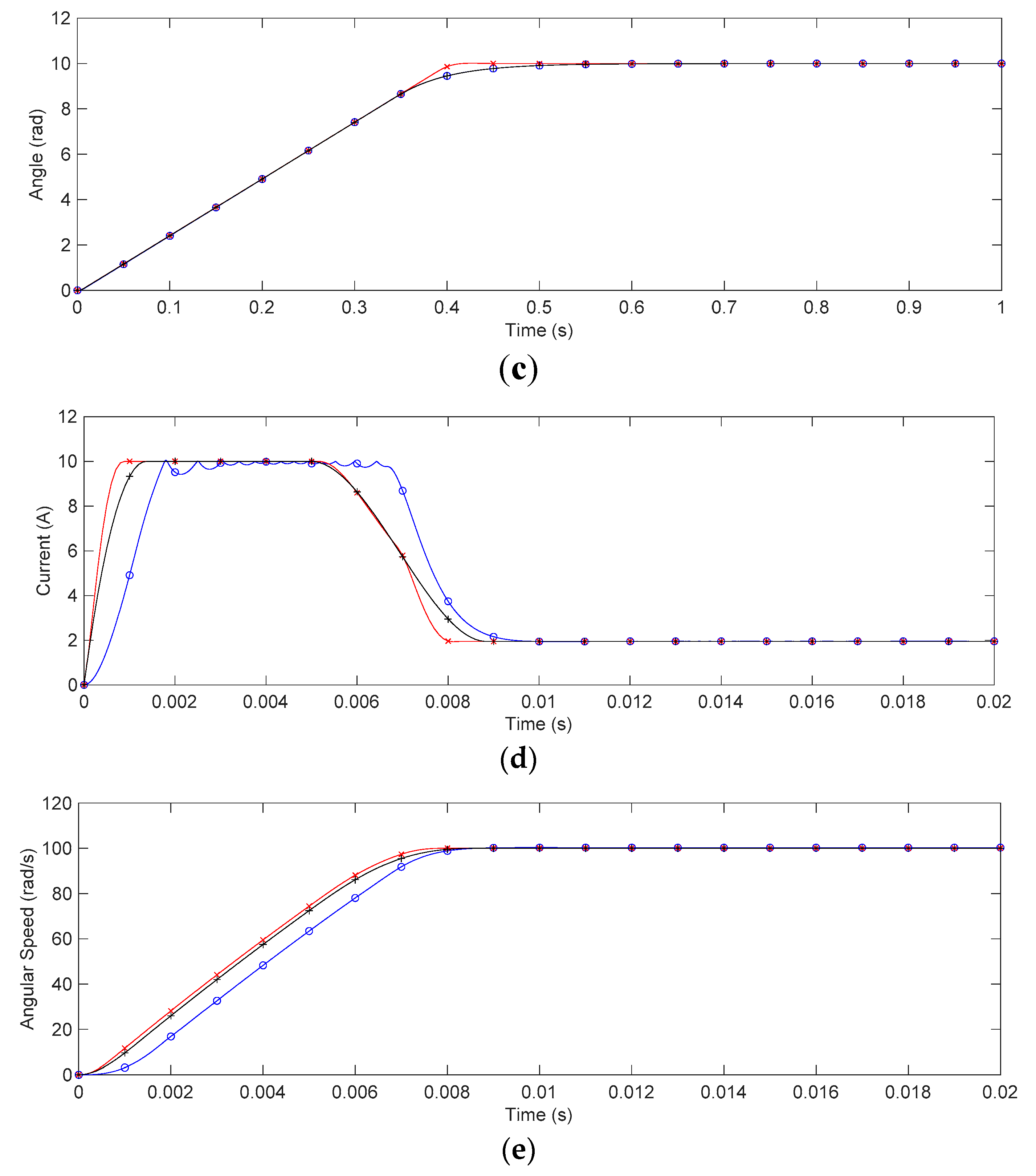
Figure 4 shows simulation results with r = 10 , x ( 0 ) = 0 , and w = [ 10 10 100 100 ] T . All other control parameters used in Figure 4 are the same as those used in Figure 3. These results show that the inequality constraints are maintained, and this leads to the conclusion that the proposed controller does not seems sensitive to r or w . The results of the implicit MPC in Figure 4a–c also differ from these of other methods therefore it is concluded that the implicit MPC differs from the optimal solution.
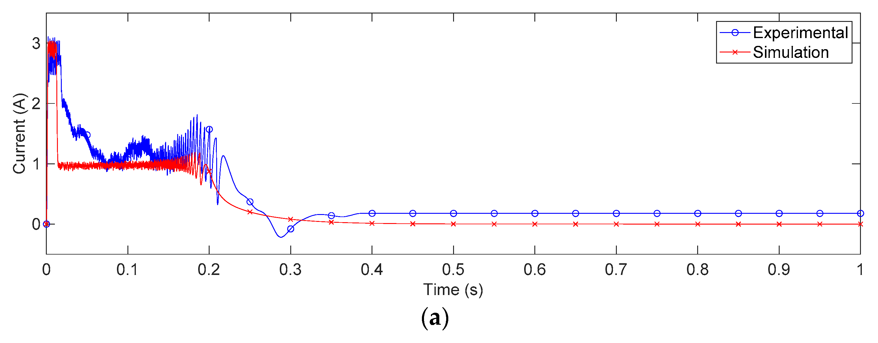
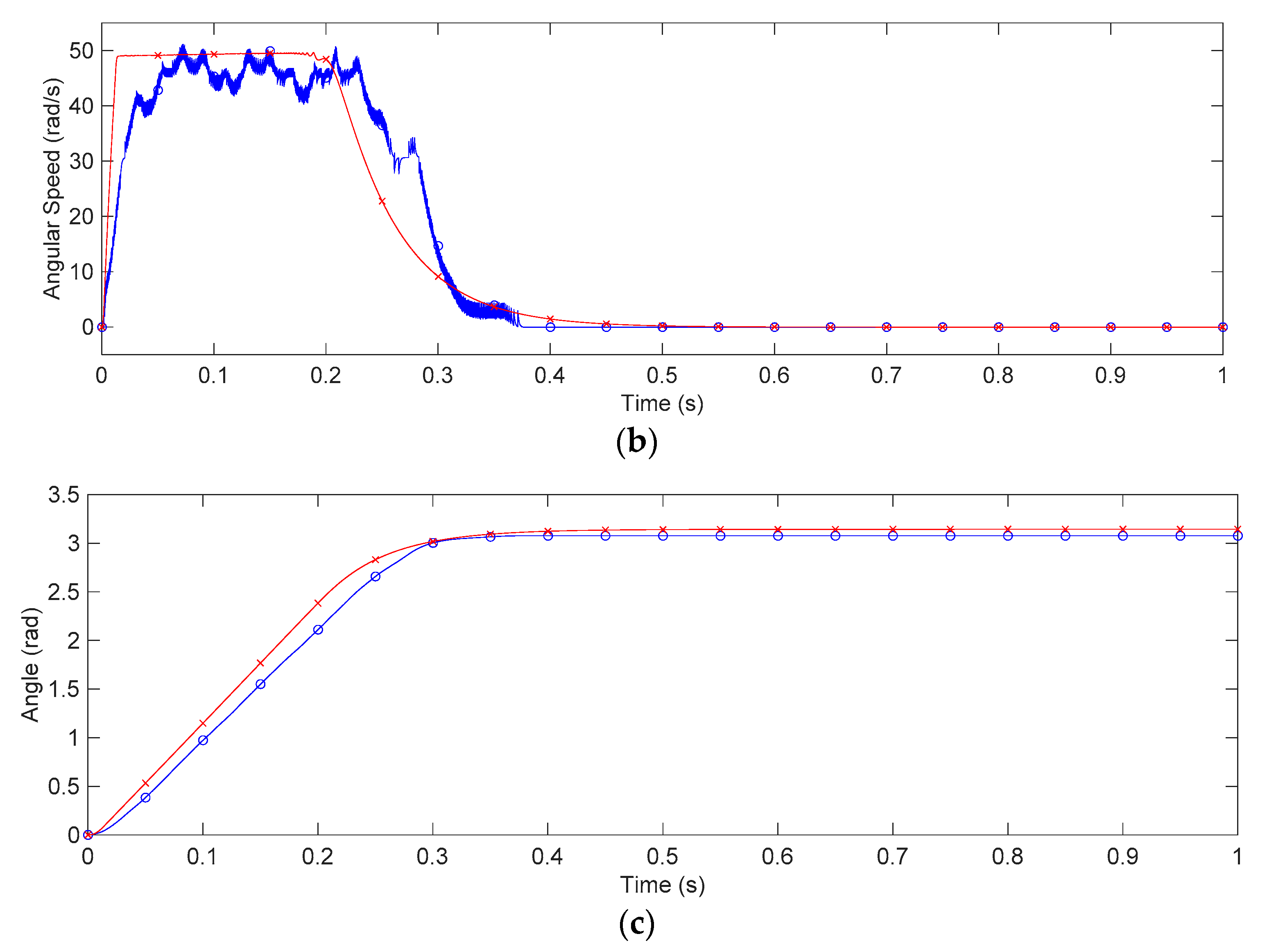
Figure 5 shows experimental and simulation results with r = π , x ( 0 ) = 0 , and w = [ 3 3 50 50 ] T . All other control parameters used in Figure 5 are the same as those used in Figure 3. Texas Instruments LAUNCHXL2-570LC43 and BOOSTXL-DRV8323RS (Dallas, TX, USA) are used to control the target motor, and they are shown in Figure 6b. The target motor is equipped with an incremental encoder as shown in Figure 6a, and the encoder has resolutions of 0.0879 degrees. The controller was designed to have sampling time of 100 μs, implemented by using Simulink® blocks, and converted to C code by using Embedded Coder® software and Embedded Coder® support package for ARM® Cortex®-R processors. For comparison, simulations were also performed at the same sampling time in Figure 5. The experimental and simulation results have similar trends in Figure 5, but the experimental results have severe vibrations and performance degradations. Since the real motor has nonlinearities and frictions, it seems that these uncertainties are related to the performance degradations.

5. Discussion

In this paper, we proposed a sub-optimal tracking controller that does not need numerical iterations or backward calculations for state-constrained optimal tracking problems. The main advantage of the proposed controller is that it can be implemented in real time with a lower computational load compared to the implicit MPC. Though there is a delay compared to the results of the numerical method, the simulation results show that the proposed controller has acceptable performance. However, the proposed controller needs to be verified through more application cases including industrial robots, hybrid vehicles, or other control systems. For future work, the proposed controller may be extended to discrete-time systems. Therefore, studies related to the discrete-time optimal tracking controller based on the proposed method are worth researching. In particular, the controller may be applied to path tracking control for autonomous vehicles [37,38], which have recently been the subject of much research.

Author Contributions

Conceptualization, J.K. and U.J.; methodology, J.K.; validation, J.K. and U.J.; writing—original draft, J.K.; writing—review and editing, U.J. and H.L.; supervision, H.L. All authors have read and agreed to the published version of the manuscript.

Funding

This research received no external funding.

Acknowledgments

This work was supported by the research fund of Hanyang University (HY-2017) and “The Technology Innovation Program” (10052501, development of design technology for a device visualizing the virtual driving environment and synchronizing with the actual vehicle driving conditions to test and evaluate ADAS), funded by the Ministry of Trade, Industry, and Energy (MI, Korea).

Conflicts of Interest

The authors declare no conflict of interest.

Appendix A

Theorem A1 
(Variational approach) [6]. Suppose that the cost function is
J = t 0 t f L ( x , x ˙ , u , λ ) d t .
Assume that the initial value and the final value of the state are fixed. Then, the necessary conditions for minimizing (A1) are
L x d d t ( L x ˙ ) = 0 ,
L u = 0 ,
L λ = 0 .
Proof. 
See Section 2.5 of [6] (pp. 169–171). □
Corollary A1: 
Suppose that the cost function is
J = t 0 t f L ( x , x ˙ , u ) d t .
Let the Hamiltonian function be
H ( x , u ) = L ( x , x ˙ , u ) + λ T x ˙ .
Then, the necessary conditions for minimizing (A5) are
λ ˙ = ( H x ) T ,
0 = H u ,
x ˙ = ( H λ ) T .
Proof
By Theorem A1,
L x d d t ( L x ˙ ) = H x + d d t ( λ T ) = H x + λ ˙ T = 0 ,
L u = H u = 0 ,
L λ = H λ x ˙ T = 0 .
Therefore, (A6) and (A7) holds. □

References

  1. Rubio, F.; Llopis-Albert, C.; Valero, F.; Suñer, J.L. Industrial robot efficient trajectory generation without collision through the evolution of the optimal trajectory. Robot. Auton. Syst. 2016, 86, 106–112. [Google Scholar] [CrossRef] [Green Version]
  2. Ragaglia, M.; Zanchettin, A.M.; Rocco, P. Trajectory generation algorithm for safe human-robot collaboration based on multiple depth sensor measurements. Mechatronics 2018, 55, 267–281. [Google Scholar] [CrossRef]
  3. Hung, C.W.; Vu, T.V.; Chen, C.K. The development of an optimal control strategy for a series hydraulic hybrid vehicle. Appl. Sci. 2016, 6, 93. [Google Scholar] [CrossRef]
  4. Guo, L.; Gao, B.; Gao, Y.; Chen, H. Optimal energy management for HEVs in eco-driving applications using bi-level MPC. IEEE Trans. Intell. Transp. Syst. 2016, 18, 2153–2162. [Google Scholar] [CrossRef]
  5. Chen, Z.; Hu, H.; Wu, Y.; Xiao, R.; Shen, J.; Liu, Y. Energy management for a power-split plug-in hybrid electric vehicle based on reinforcement learning. Appl. Sci. 2018, 8, 2494. [Google Scholar] [CrossRef] [Green Version]
  6. Kirk, D.E.; Donald, E. Optimal Control Theory: An Introduction; Dover Publications: Mineola, NY, USA, 2004; pp. 53–239. [Google Scholar]
  7. Athans, M.; Falb, P.L. Optimal Control: An Introduction to the Theory and Its Applications; Dover Publications: Mineola, NY, USA, 2007; pp. 221–812. [Google Scholar]
  8. Lewis, F.L.; Vrabie, D.; Syrmos, V.L. Optimal Control, 3rd ed.; John Wiley & Sons: Hoboken, NJ, USA, 2012; pp. 110–212. [Google Scholar]
  9. Pontryagin, L.S. Mathematical Theory of Optimal Processes; John Wiley & Sons: Hoboken, NJ, USA, 1962; pp. 9–114. [Google Scholar]
  10. Elbert, P.; Ebbesen, S.; Guzzella, L. Implementation of dynamic programming for n-dimensional optimal control problems with final state constraints. IEEE Trans. Control Syst. Technol. 2012, 21, 924–931. [Google Scholar] [CrossRef]
  11. Böhme, T.J.; Frank, B.J.C. Hybrid Systems, Optimal Control and Hybrid Vehicles; Springer International: Cham, Switzerland, 2017; pp. 167–270. [Google Scholar]
  12. Betts, J.T. Survey of numerical methods for trajectory optimization. J. Guidance Control. Dyn. 1998, 21, 193–207. [Google Scholar] [CrossRef]
  13. Betts, J.T. Practical Methods for Optimal Control and Estimation Using Nonlinear Programming, 2nd ed.; Society for Industrial and Applied Mathematics: Philadelphia, PA, USA, 2010; pp. 96–218. [Google Scholar]
  14. Mayne, D.Q.; Rawlings, J.B.; Rao, C.V.; Scokaert, P.O. Constrained model predictive control: Stability and optimality. Automatica 2000, 36, 789–814. [Google Scholar] [CrossRef]
  15. Qin, S.J.; Badgwell, T.A. A survey of industrial model predictive control technology. Control Eng. Pract. 2003, 11, 733–764. [Google Scholar] [CrossRef]
  16. Wang, L. Model Predictive Control System Design and Implementation Using MATLAB®; Springer-Verlag: London, UK, 2009; pp. 1–224. [Google Scholar]
  17. Aldaouab, I.; Daniels, M.; Ordóñez, R. MPC for optimized energy exchange between two renewable-energy prosumers. Appl. Sci. 2019, 9, 3709. [Google Scholar] [CrossRef] [Green Version]
  18. Bemporad, A.; Morari, M.; Dua, V.; Pistikopoulos, E.N. The explicit linear quadratic regulator for constrained systems. Automatica 2002, 38, 3–20. [Google Scholar] [CrossRef]
  19. Bemporad, A.; Borrelli, F.; Morari, M. Model predictive control based on linear programming—The explicit solution. IEEE Trans. Autom. Control. 2002, 47, 1974–1985. [Google Scholar] [CrossRef]
  20. Grancharova, A.; Johansen, T.A. Explicit Nonlinear Model Predictive Control: Theory and Applications; Springer-Verlag: London, UK, 2012; pp. 1–108. [Google Scholar]
  21. Bemporad, A.; Morari, M.; Dua, V.; Pistikopoulos, E.N. Corrigendum to: “The explicit linear quadratic regulator for constrained systems” [Automatica 38 (1)(2002) 3–20]. Automatica 2003, 39, 1845–1846. [Google Scholar] [CrossRef]
  22. Franklin, G.F.; Powell, J.D.; Workman, M. Digital Control of Dynamic Systems, 3rd ed.; Addison-Wesley: Menlo Park, CA, USA, 1998; pp. 96–118. [Google Scholar]
  23. Venkataraman, P. Applied Optimization with MATLAB Programming; John Wiley & Sons: Hoboken, NJ, USA, 2002; pp. 265–316. [Google Scholar]
  24. Bryson, A.E. Applied Optimal Control: Optimization, Estimation and Control; Hemisphere Publishing Corporation: Washington, DC, USA, 1975; pp. 212–245. [Google Scholar]
  25. Zhang, X.D. Matrix Analysis and Applications; Cambridge University Press: Cambridge, UK, 2017; pp. 60–61. [Google Scholar]
  26. Bernstein, D.S. Matrix Mathematics: Theory, Facts, and Formulas, 2nd ed.; Princeton university press: Princeton, NJ, USA, 2009; pp. 77–164. [Google Scholar]
  27. Khalil, H.K.; Grizzle, J.W. Nonlinear Systems, 3rd ed.; Prentice-Hall: Upper Saddle River, NJ, USA, 2002; pp. 111–194. [Google Scholar]
  28. Chen, C.T. Linear System Theory and Design, 3rd ed.; Oxford University Press: Oxford, UK, 1998; pp. 121–140. [Google Scholar]
  29. Lin, C.Y.; Liu, Y.C. Precision tracking control and constraint handling of mechatronic servo systems using model predictive control. IEEE/ASME Trans. Mechatron. 2011, 17, 593–605. [Google Scholar]
  30. Rădac, M.B.; Precup, R.E.; Petriu, E.M.; Preitl, S.; Dragoş, C.A. Data-driven reference trajectory tracking algorithm and experimental validation. IEEE Trans. Ind. Inf. 2012, 9, 2327–2336. [Google Scholar] [CrossRef]
  31. Premkumar, K.; Manikandan, B.V.; Kumar, C.A. Antlion algorithm optimized fuzzy PID supervised on-line recurrent fuzzy neural network based controller for brushless DC motor. Electr. Power Compon. Syst. 2017, 45, 2304–2317. [Google Scholar] [CrossRef]
  32. Hassan, A.K.; Saraya, M.S.; Elksasy, M.S.; Areed, F.F. Brushless DC motor speed control using PID controller, fuzzy controller, and neuro fuzzy controller. Int. J. Comput. Appl. 2018, 180, 47–52. [Google Scholar]
  33. Sun, Z.; Pritschow, G.; Zahn, P.; Lechler, A. A novel cascade control principle for feed drives of machine tools. CIRP Ann. 2018, 67, 389–392. [Google Scholar] [CrossRef]
  34. Guerra, R.H.; Quiza, R.; Villalonga, A.; Arenas, J.; Castaño, F. Digital twin-based optimization for ultraprecision motion systems with backlash and friction. IEEE Access 2019, 7, 93462–93472. [Google Scholar] [CrossRef]
  35. Andersson, J.A.; Gillis, J.; Horn, G.; Rawlings, J.B.; Diehl, M. CasADi: A software framework for nonlinear optimization and optimal control. Math. Program. Comput. 2019, 11, 1–36. [Google Scholar] [CrossRef]
  36. Anderson, B.D.; Moore, J.B. Optimal Control: Linear Quadratic Methods; Dover Publications: Mineola, NY, USA, 1990; pp. 68–100. [Google Scholar]
  37. Yao, Q.; Tian, Y. A model predictive controller with longitudinal speed compensation for autonomous vehicle path tracking. Appl. Sci. 2019, 9, 4739. [Google Scholar] [CrossRef] [Green Version]
  38. Wu, X.; Qiao, B.; Su, C. Trajectory planning with time-variant safety margin for autonomous vehicle lane change. Appl. Sci. 2020, 10, 1626. [Google Scholar] [CrossRef] [Green Version]
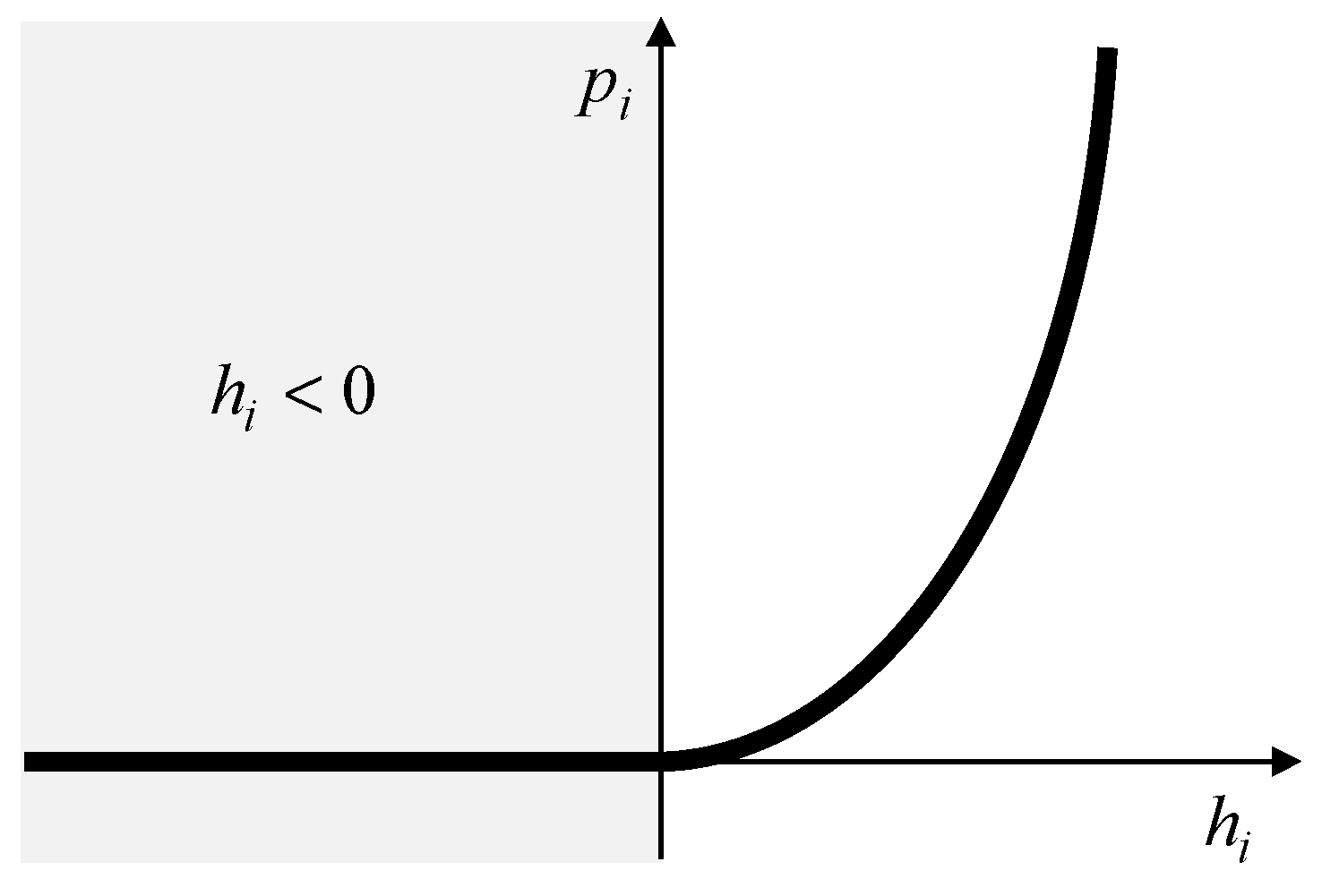
Figure 1. An example of the penalty function (15).
Applsci 10 05724 g001
Figure 2. Modified plant model with a low-pass filter.
Applsci 10 05724 g002
Figure 3. Simulation results of the proposed controller, the numerical method, and the implicit MPC with the first set of r and w: (a) motor currents from 0 to 1 s, (b) angular speeds of the motor rotor from 0 to 1 s, (c) angle of the motor rotor from 0 to 1 s, (d) motor currents from 0 to 0.02 s, (e) angular speeds of the motor rotor from 0 to 0.02 s.
Applsci 10 05724 g003aApplsci 10 05724 g003b
Figure 4. Simulation results of the proposed controller, the numerical method, and the implicit MPC with the second set of r and w: (a) motor currents from 0 to 1 s, (b) angular speeds of the motor rotor from 0 to 1 s, (c) angle of the motor rotor from 0 to 1 s, (d) motor currents from 0 to 0.02 s, (e) angular speeds of the motor rotor from 0 to 0.02 s.
Applsci 10 05724 g004aApplsci 10 05724 g004b
Figure 5. Experimental and simulation results of the proposed controller with 100 μs sampling time and the first set of r and w: (a) motor currents from 0 to 1 s, (b) angular speeds of the motor rotor from 0 to 1 s, (c) angle of the motor rotor from 0 to 1 s.
Applsci 10 05724 g005aApplsci 10 05724 g005b
Figure 6. Target motor and controller: (a) motor, (b) controller.
Applsci 10 05724 g006
Table 1. The parameters of the target motor.
NameUnitValue
Rotor inductance ( L m )H0.0065
Armature resistance ( R m )Ω2.3
Back EMF constant ( K b )V·sec/rad0.09
Torque constant ( K m )Nm/A0.09
Friction coefficient ( B m )Nm·sec0.00175
Rotor inertia ( J m )Nm·rad0.0000525
Gear ratio ( κ m ) 0.25
Table 2. Examples of the solutions of (34).
α x P s α x P s
[ 0 0 0 0 ] [ 0.08 0.02 6.50 0.01 * 0 1.46 0 * * 555.69 1 * * * 0 ] [ 10000 0 0 0 ] [ 12.21 0.13 6.63 1.29 * 0.06 1.56 0.04 * * 561.18 1 * * * 0.20 ]
[ 0 10000 0 0 ] [ 12.21 0.13 6.63 1.29 * 0.06 1.56 0.04 * * 561.18 1 * * * 0.20 ] [ 0 0 0.001 0 ] [ 0.08 0.02 6.50 0.01 * 0 1.46 0 * * 555.69 1 * * * 0 ]
[ 10000 0 0.001 0 ] [ 12.21 0.13 6.63 1.29 * 0.06 1.56 0.04 * * 561.18 1 * * * 0.20 ] [ 0 10000 0.001 0 ] [ 12.21 0.13 6.63 1.29 * 0.06 1.56 0.04 * * 561.18 1 * * * 0.20 ]
[ 0 0 0 0.001 ] [ 0.08 0.02 6.50 0.01 * 0 1.46 0 * * 555.69 1 * * * 0 ] [ 10000 0 0 0.001 ] [ 12.21 0.13 6.63 1.29 * 0.06 1.56 0.04 * * 561.18 1 * * * 0.20 ]
[ 0 10000 0 0.001 ] [ 12.21 0.13 6.63 1.29 * 0.06 1.56 0.04 * * 561.18 1 * * * 0.20 ]