A Novel Hybrid Decomposition—Ensemble Prediction Model for Dam Deformation

Abstract

Accurate and reliable prediction of dam deformation (DD) is of great significance to the safe and stable operation of dams. In order to deal with the fluctuation characteristics in DD for more accurate prediction results, a new hybrid model based on a decomposition-ensemble model named VMD-SE-ER-PACF-ELM is proposed. First, the time series data are decomposed into subsequences with different frequencies and an error sequence (ER) by variational mode decomposition (VMD), and then the secondary decomposition method is introduced into the prediction of ER. In these two decomposition processes, the sample entropy (SE) method is innovatively utilized to determine the decomposition modulus. Then, the input variables of the subsequences are selected by partial autocorrelation analysis (PACF). Finally, the parameter-optimization-based extreme learning machine (ELM) models are used to predict the subsequences, and the outputs are reconstructed to obtain the final prediction results. The case analysis shows that the VMD-SE-ER-PACF-ELM model has strong prediction ability for DD. The model is then compared with other nonlinear and time series models, and its performance under different prediction periods is also analyzed. The results show that the proposed model is able to adequately describe the original DD. It performs well in both training and testing stages. It is a preferred data-driven model for DD prediction and can provide a priori knowledge for health monitoring of dams.

1. Introduction

Dams can bring significant socio-economic benefits under safe operating conditions. In case of a dam accident, there will be a huge disaster [1,2,3]. In fact, most dam accidents did not arise suddenly, but went through a process from quantity to quality variation [4]. If we can establish suitable prediction models for dam monitoring data and analyze them in a timely manner, potential problems in the structural behavior of dams will be identified, thus avoiding accidents.

As the controlled indicator of dam safety monitoring, deformation monitoring data can objectively reflect the structural state and the safety condition of dams, which are one of the important bases for assessing the safety of dam projects [5]. During the actual service of a dam, the deformation monitoring data are usually complex nonstationary and nonlinear time series. Therefore, it is an important research topic to accurately predict dam deformation (DD) in the future by using historical deformation monitoring data [6,7]. Currently, the commonly used models for predicting DD are the deterministic models, statistical models, neural network models, and hybrid models [7,8,9,10,11,12,13].

The deterministic models explain DD based on the physical laws of loads, material properties, and stress–strain relationships [6,14], requiring as accurate as possible material parameters, geometry, and operating conditions of the dam and its foundation, which are difficult to achieve in actual engineering [15,16]. In contrast, a statistical model is more easily implemented [13]. It is a more commonly used data-driven approach for DD monitoring [17]. Although the statistical model is simple and effective, it cannot capture the nonlinear characteristics of the DD time series, thus affecting the accuracy of deformation prediction [14]. In comparison, a neural network model has unique advantages in dealing with nonlinear problems [18,19]. In the field of DD prediction, the neural network models have good and robust prediction performance. This so-called ‘black box’ method can build a data-driven model based on the historical deformation data of dams, thereby achieving high-precision prediction of deformation without knowing detailed environmental information, avoiding complex data handling and modeling processes. Among them, the artificial neural networks (ANN) [20] and support vector machines (SVM) [21] are the most commonly used methods for the nonlinear problems. However, these models have some limitations [5]. An ANN model based on gradient descent requires multiple iterations to correct the relevant parameters, which is a time-consuming process and the model tends to fall into local minima. Although an SVM overcomes the shortcomings of the ANN model, its kernel function parameters are difficult to choose [1]. Therefore, in this paper, the extreme learning machine (ELM) [22,23,24] with efficient regression capabilities is chosen as the basic model for DD prediction to address the drawbacks of the above models [25,26]. It randomly generates connection weights between the input and hidden layers and thresholds for neurons in the hidden layer without adjusting during the training process. The conditions for the unique optimal solution of the ELM output are the determined activation function and the hidden layer parameters. Compared with traditional methods, ELMs have the advantages of fast learning speed and good generalization performance [27].

Although the ELM model has some advantages for handling nonlinear problems, the strong volatility of the deformation data will undoubtedly have negative impacts on the prediction results. Therefore, before predicting the DD, we need to preprocess the time series by signal decomposition technique, which can extract useful information from the original data to improve the prediction accuracy of data-driven models. Wavelet decomposition (WD) and empirical modal decomposition (EMD) are two common signal decomposition techniques [1,28,29,30,31], and they are widely used in the processing of strongly fluctuating data. However, they have certain drawbacks, such as the difficulty in choosing wavelet bases and decomposition scales in wavelet transforms, and the basic disadvantage of EMD is the lack of mathematical foundation. To address these issues, the variational mode decomposition (VMD) [32] algorithm is introduced in this study. Compared with EMD, WD, and other methods, VMD is an accurate mathematical model, which can decompose the original data into a set of variational mode functions (VMFs) that fluctuate around the center frequency [33,34,35], with better decomposition effect and higher robustness [36,37,38]. Currently, the contribution of VMD in the field of prediction has now been confirmed by some scholars, such as energy power generation prediction [39], carbon price prediction [40], runoff prediction [41], container throughput prediction [42] and air quality index prediction [43]. However, to the best of the authors’ knowledge, the application for DD prediction has not been extensively explored, so this study will provide a priori knowledge for the utilization of VMD in dam safety monitoring.

In practical applications, the decomposition effect of VMD is affected by the decomposition modulus K. If the K value is too small, the obtained VMFs will lose information; on the contrary, it will lead to excessive decomposition and even make the decomposition results worse [44,45]. In paper [41], the decomposition modulus was determined by central frequency. Here, we propose a more efficient method for determining the decomposition modulus—sample entropy (SE) method. The SE can characterize the complexity of the time series, and when the time series is perturbed and the uncertainty of its state value increases, the value of the SE will also increase accordingly [46]. If two or more subsequences have similar SE values, modal confusion occurs in the decomposition. Therefore, in this paper, we choose the maximum K value that allows a large difference between the SE values of any two subsequences as the final decomposition modulus of the VMD. In addition, there is an error sequence (ER) between the sum of the subsequences obtained by the VMD algorithm and the original sequence. In other words, the sum of the VMFs is not equal to the original sequence [47]. Since the ER contains the true fluctuation characteristics of the original sequence, considering only VMFs will not fully reflect the randomness, which will lead to distortion of the prediction results to some extent. In this paper, the ER of the DD after decomposition is extracted, and because the sequence is approximately noisy, it cannot be modeled directly using the machine learning model to obtain good prediction results. To solve this problem, the authors of paper [47] proposed the random number method for point prediction of ER, but the uncertainty of the results obtained by this method is significant. Therefore, we innovatively propose a VMD-based secondary decomposition for the ER in order to dig deeper into the temporal features embedded in it. The results show that the prediction obtained by considering the ER is closer to the observed values and has more practical engineering significance.

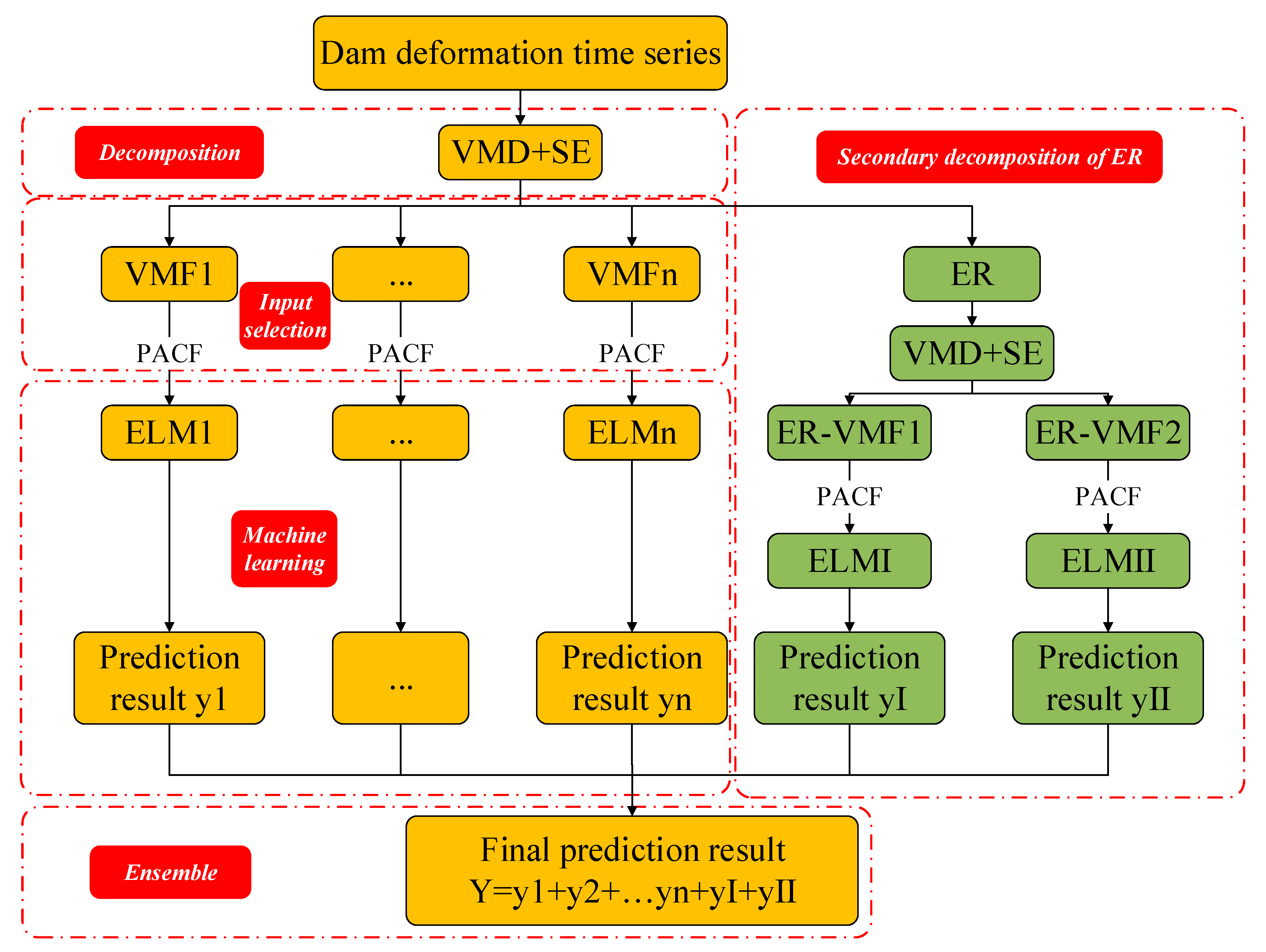
In summary, a hybrid model, namely VMD-SE-ER-PACF-ELM, for the DD prediction is proposed, which makes full use of the advantages of the VMD, SE, PACF, and ELM neural network. First, the VMD-SE model is used to decompose a deformation sequence into K VMFs with good characteristics and an ER. For the ER, the same method is used to obtain a series of subsequences. Secondly, the partial autocorrelation function (PACF) method is used to determine the input variables of the subsequences. Then the ELM models corresponding to each subsequence is trained in the machine-learning process. Finally, the ELMs are applied to the corresponding subsequences, and the sum of the prediction results of each component is the final result of the DD prediction. Meanwhile, comparisons are made between the model and other prediction models, while validating it through different prediction periods.

The rest of this paper is organized as follows: Section 2 briefly introduces the methods mentioned above. In Section 3, the proposed model and performance evaluation indicators are introduced. Then, in Section 4, a case study and discussion of the results are presented, and Section 5 presents the conclusions of the study.

2. Methodology

2.1. VMD Based Decomposition Method

VMD is a completely new, non-recursive signal decomposition method proposed by Dragomiretskiy et al. in 2014 [32]. It can decompose any signal $f\left(t\right)$ into K modal components $u_k$ around the center frequency ${\omega }_k$. For the VMD algorithm, the signal decomposition process is solving a variable division problem, which is modeled as follows

$$\{\begin{array}{c}\begin{array}{c}min\\ \left\{u_k\right\},\left\{{\omega }_k\right\}\end{array}=\left\{{\displaystyle {\displaystyle \sum }_k}\left|\right|{\partial }_t\left[\left(\delta \left(t\right)+\frac{j}{\pi t}\right)u_k\left(t\right)\right]\ast e^{-j{\omega }_{k}t}{\left|\right|}_2^2\right\}\\ {\displaystyle {\displaystyle \sum }_k}{u}_k=f\end{array}$$

(1)

where $\left\{u_k\right\}=\left\{u_1,u_2,\cdots u_k\right\}$ are the K modal components, $\left\{{\omega }_k\right\}=\left\{{\omega }_1,{\omega }_2\cdots {\omega }_k\right\}$ are the center frequency of each modal component, $f$ is the original signal, and ${\delta }_t$ is the pulse function. In order to obtain the optimal solution of the constrained variational problem, the Lagrange multiplication operator $\lambda \left(t\right)$ and the quadratic penalty factor $a$ are introduced to transform the constrained variational problem into an unconstrained variational problem. The extended Lagrange function is expressed as

$$L\left(\left\{u_k\right\},\left\{{\omega }_k\right\},\lambda \right)=a{\displaystyle \sum }_k\left|\right|{\partial }_t\left[\left(\delta \left(t\right)+\frac{j}{\pi t}\right)u_k\left(t\right)\right]\ast e^{-j{\omega }_{k}t}{\left|\right|}_2^2+\left|\right|f\left(t\right)-{\displaystyle \sum }_k{u}_k{\left(t\right)\left|\right|}_2^2+\langle \lambda \left(t\right),f\left(t\right)-{\displaystyle \sum }_k{u}_k\left(t\right)\rangle$$

(2)

The optimal solution of Equation (2) is obtained by updating $u_k^{n+1}$, ${\omega }_k^{n+1}$ and ${\lambda }_k^{n+1}$ with alternating direction operator multiplication algorithm. The iterative equations are as follows

$${\widehat{u}}_k^{n+1}\left(\omega \right)=\frac{\widehat{f}\left(\omega \right)-{{\displaystyle \sum }}_{i<k}{\widehat{u}}_i^{n+1}\left(\omega \right)+{\widehat{\lambda }}^n\left(\omega \right)/2}{1+2a{\left(\omega -{\omega }_k^n\right)}^2}$$

(3)

$${\omega }_k^{n+1}=\frac{{{\displaystyle \int }}_0^{\infty }\omega {\left|{\widehat{u}}_k^{n+1}\left(\omega \right)\right|}^{2}d\omega }{{{\displaystyle \int }}_0^{\infty }{\left|{\widehat{u}}_k^{n+1}\left(\omega \right)\right|}^{2}d\omega }$$

(4)

$${\widehat{\lambda }}^{n+1}\left(\omega \right)={\widehat{\lambda }}^n+\tau (\widehat{f}\left(\omega \right)-{\displaystyle \sum }_k{\widehat{u}}_k^{n+1}\left(\omega \right))$$

(5)

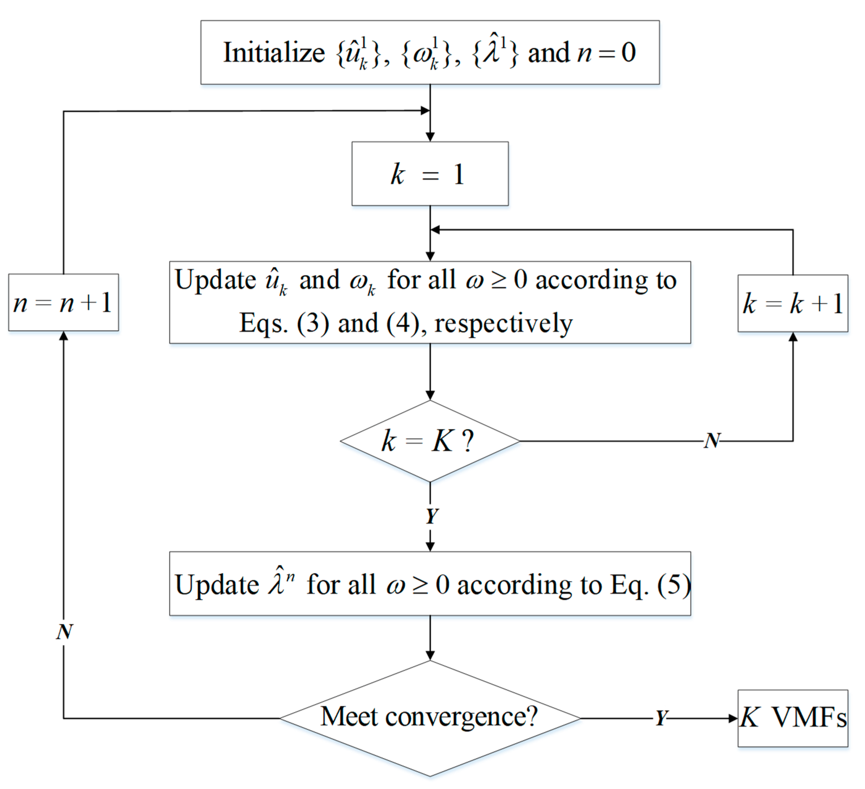
In Equations (3)–(5), ${\widehat{u}}_k^{n+1}\left(\omega \right), \widehat{f}\left(\omega \right)$ and ${\widehat{\lambda }}^{n+1}\left(\omega \right)$ represent the Fourier transforms corresponding to $u_k^{n+1}\left(\omega \right)$, $f\left(\omega \right)$ and ${\lambda }^{n+1}\left(\omega \right)$ respectively. The constraints for iterative stop are

$$\frac{{{\displaystyle \sum }}_k\left|\right|{\widehat{u}}_k^{n+1}-{\widehat{u}}_k^n{\left|\right|}_2^2}{\left|\right|{\widehat{u}}_k^n{\left|\right|}_2^2}<\epsilon$$

(6)

Above all, the specific procedures of VMD are shown in Figure 1.

2.2. SE Based Modulus Selection Method

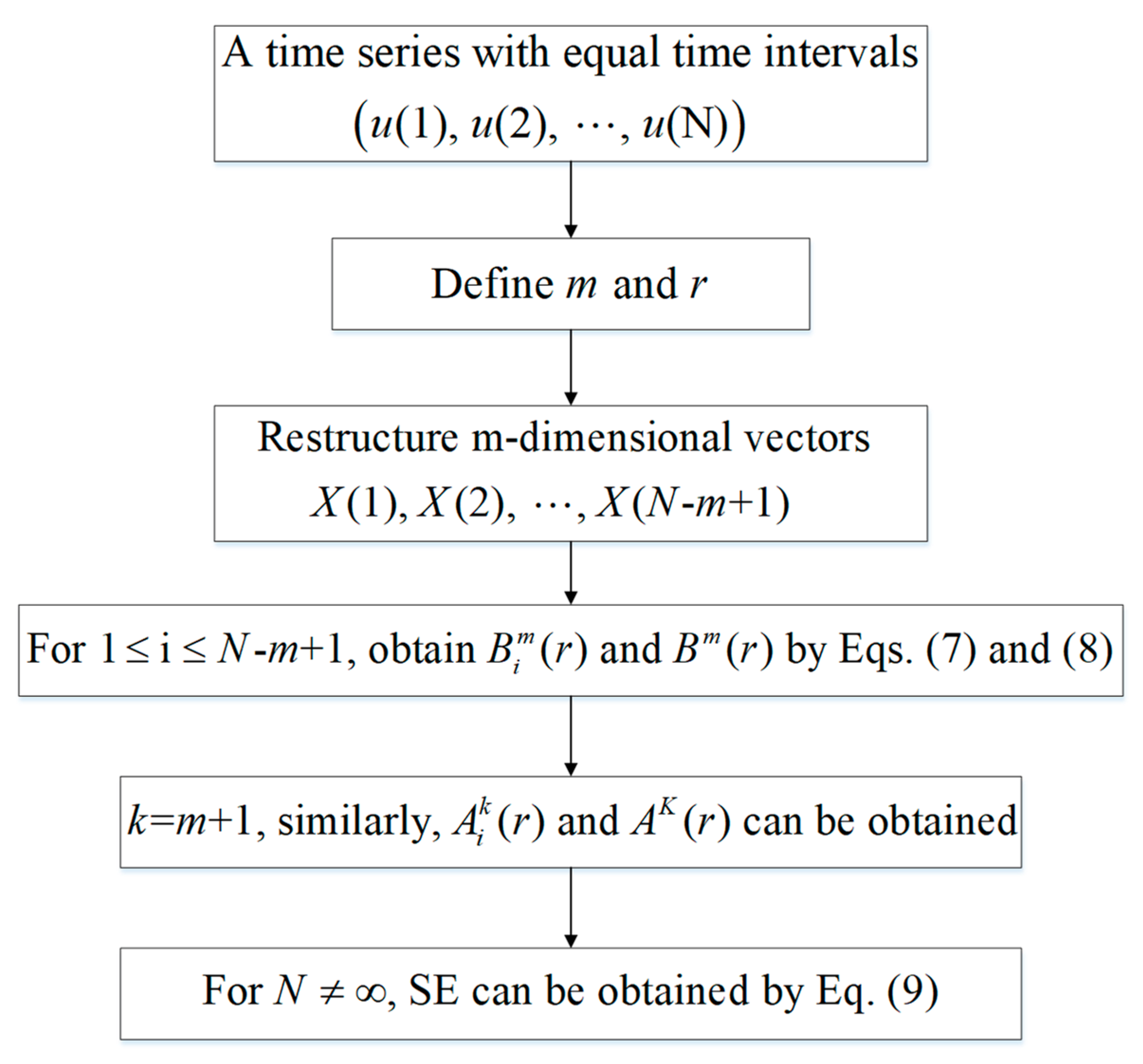
When using the VMD algorithm, the decomposition modulus can be set in advance. By setting reasonable convergence conditions, the computational complexity of the model can be effectively reduced [41]. A new method for determining the modulus K using the SE values of the VMFs is proposed. The concept of SE was introduced by Richman et al. in 2000 [48], and it is used to evaluate the complexity of time series. The higher self-similarity of the time series means the smaller SE value, and vice versa [49]. After the decomposition of the DD time series, a number of subsequences and their corresponding SE values can be obtained. If there are two or more subsequences with similar SE values, it is assumed that over-decomposition occurs, which leads to modal confusion; if the SE values of the VMFs are quite different from each other, the maximum K value that allows this state should be selected as the final decomposition modulus to avoid under-decomposition of the VMD. The specific process of SE is illustrated in Figure 2.

In Figure 2, Equations (7)–(9) are as follows

$$B_i^m\left(r\right)=\frac{number of X\left(j\right) such that d\left[X\left(i\right),X\left(j\right)\right]\le r}{N-m}, i\ne j$$

(7)

$$B^m\left(r\right)={\left(N-m+1\right)}^{-1}{\displaystyle \sum }_{i=1}^{N-m+1}{B}_i^m\left(r\right)$$

(8)

$$SE=-\ln \left[A^k\left(r\right)/B^m\left(r\right)\right]$$

(9)

where $m$ is an integer that represents the length of the comparison vector, $r$ is a real number indicating the measure of similarity, $X\left(i\right)=\left[u\left(i\right),u\left(i+1\right),\cdots ,u\left(i+m-1\right)\right]$, $d\left[X,X*\right]$ is defined as $d\left[X,X*\right]=max\left|u\left(a\right)-u*\left(a\right)\right|, X\ne X*$, $u\left(a\right)$ is the element of vector $X$, $d$ represents the distance between vectors $X\left(i\right)$ and $X\left(j\right)$, and the value of $j$ is in the range $\left[1,N-m+1\right]$.

As shown in Figure 2, the values of $m$ and $r$ need to be determined before calculating the SE. Typically, values of the embedding dimension $m$ are taken as 1 or 2. The selection of a similar tolerance $r$ depends largely on the practical application scenario, usually $=0.1\ast std~0.25std$, where std is the standard deviation of the original data. In the paper, set $m=2$ and $r=0.2\ast std$.

2.3. PACF Based Input Selection Method

Due to the different fluctuation characteristics of the DD at different periods, the correlations of the K VMFs obtained by the above method also vary. Therefore, before predicting each component, we need to analyze the correlation of each VMF, and then the optimal input variables for the ELMs can be selected. Here, the PACF method is used to evaluate the correlations and selection results of the components [50].

Assume that $X_t$ is the output variable, and if the lag autocorrelation length value of $X_{t-a}$ falls at the 95% confidence interval $\left[-\frac{1.96}{\sqrt{n}},\frac{1.96}{\sqrt{n}}\right]$ for the first time, and there are no obvious outliers after it. At this time, $\left(a-1\right)d$ is selected as the delay time value of the corresponding time series. PACF is described below.

For DD time series, the covariance ${\widehat{\gamma }}_a$ at lag $a$ is expressed as

$${\widehat{\gamma }}_a=\frac{1}{n}{\displaystyle \sum }_{t=1}^{n-a}\left(x_t-\widehat{x}\right)\left(x_{t+a}-\overline{x}\right),\hspace{1em}\left(a=1,2,\cdots ,M\right)$$

(10)

where $\overline{x}$ is the mean value of the time series and $M$ is the largest lag coefficient, $a$ is the lag length of the autocorrelation function, and ${\widehat{\rho }}_a$ can be estimated as follows

$${\widehat{\rho }}_a={\widehat{\gamma }}_a/{\widehat{\gamma }}_0$$

(11)

For PACF at lag $a$, the $f_{aa}$ is presented as follows

$$\{\begin{array}{c}{\widehat{f}}_{11}={\widehat{\rho }}_1\\ {\widehat{f}}_{a+1,a+1}=\left({\widehat{\rho }}_{a+1}-{{\displaystyle \sum }}_{j=1}^a{\widehat{\rho }}_{a+1-j}{\widehat{f}}_{aj}\right)/\left(1-{{\displaystyle \sum }}_{j=1}^a{\widehat{\rho }}_j{\widehat{f}}_{aj}\right)\\ {\widehat{f}}_{a+1,j}={\widehat{f}}_{aj}-{\widehat{f}}_{a+1,a+1}{\widehat{f}}_{a,a-j+1}\end{array},\hspace{1em} \hspace{1em}\left(j=1,2,\cdots ,a\right)$$

(12)

where $1\le a\le M$.

2.4. ELM-Based Prediction Model

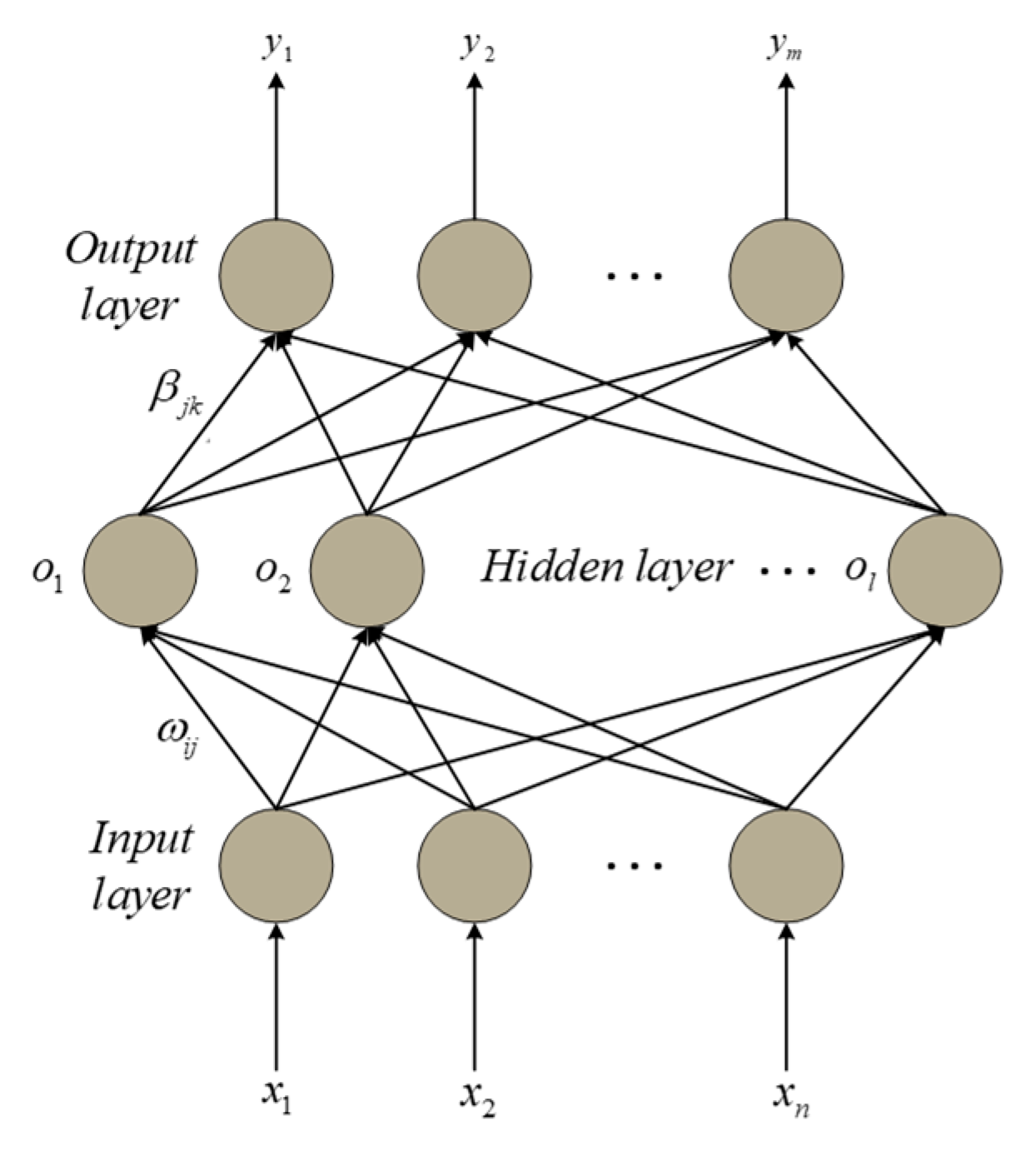
The ELM model is chosen as the core model for DD prediction in this paper, and its structure is shown in Figure 3. It is a new type of feedforward neural network [22]. Compared with the traditional single hidden layer feedforward neural networks (SLFNs), ELM has some significant advantages, such as fast training speed, good generalization ability, and few adjustable parameters. Its specific principles are as follows

Given a $Q$-group sample $\left(x_n,t_m\right)$, where $x_n={\left[x_{n1},x_{n2},\dots ,x_{nQ}\right]}^T$ and $t_m={\left[t_{m1},t_{m2},\dots ,t_{mQ}\right]}^T$. Assume that the activation function of the hidden layer neurons is $g\left(x\right)$, the output vector of the network is as follows

$$T={\left[t_1,t_2,\dots ,t_Q\right]}_{m.Q}$$

(13)

$$t_j={\left[t_{1j},t_{2j},\dots ,t_{mj}\right]}^T={\displaystyle \sum }_{i=1}^l{\beta }_{im}g\left({\omega }_i{x}_i+b_i\right)\hspace{1em} \hspace{1em}\left(j=1,2,\dots ,Q\right)$$

(14)

where $b_i$ denotes the threshold of the ith neural node of the hidden layer, ${\omega }_i={\left[{\omega }_{1i},{\omega }_{2i},\dots ,{\omega }_{mi}\right]}^T$ is the weight of the ith neural node, and ${\beta }_i={\left[{\beta }_{1i},\beta ,\dots ,{\beta }_{mi}\right]}^T$ is the weight of the ith neural node. Equation (13) can be described as Equation (15)

$$H\beta =T^{\prime }$$

(15)

where $H$ is the hidden layer output matrix, which can be represented by Equation (16)

$$H\left({\omega }_1,{\omega }_2,\dots ,{\omega }_l,b_1,b_2,\dots ,b_l,x_1,x_2,\dots ,x_Q\right)=\left[\begin{array}{ccc}g\left({\omega }_1·x_1+b_1\right)& \cdots & g\left({\omega }_l·x_1+b_l\right)\\ ⋮& \cdots & ⋮\\ g\left({\omega }_1·x_Q+b_1\right)& \cdots & g\left({\omega }_l·x_Q+b_l\right)\end{array}\right]$$

(16)

According to the ELM theorem, if $l=Q$, for arbitrary $\omega$ and $b$, Equation (17) can be obtained

$${\displaystyle \sum }_{j=1}^Q\left|\left|t_j-y_j\right|\right|=0$$

(17)

where $y_j={\left[y_{1j},y_{2j},\cdots ,y_{mj}\right]}^T \left(j=1,2,\cdots ,Q\right)$. When $Q$ is large, $l$ is usually less than $Q$ in order to reduce the amount of computation, which means that the ELM training error can be approximated to an arbitrary number $\epsilon >0$.

$${\displaystyle \sum }_{j=1}^Q\left|\left|t_j-y_j\right|\right|<\epsilon$$

(18)

The connection weight $\beta$ can be obtained as follows

$$\underset{\beta }{\min }\left|\left|H\beta -T^{\prime }\right|\right|$$

(19)

Its solution can be expressed as Equation (20)

$$\widehat{\beta }=H^{+}{T}^{\prime }$$

(20)

where $H^{+}$ is the generalized inverse Moore-Penrose matrix of the $H$ matrix.

In summary, the ELM model does not require iterative corrections to weights and thresholds, and it outperforms conventional SLFNs.

3. DD Prediction Model and Performance Evaluation Indicators

3.1. The Hybrid DD Prediction Model

In this section, we develop a new hybrid model for DD prediction based on VMD-SE-ER-PACF-ELM. The detailed steps of the proposed model are shown in Figure 4.

3.2. Performance Evaluation Indicators

In this paper, three evaluation indicators and the Taylor diagram are presented to evaluate the performance of the proposed model.

• Root mean square error (RMSE)
  RMSE is used to characterize the overall prediction precision.

  $$RMSE=\sqrt{\frac{1}{n}{\displaystyle \sum }_{i=1}^n{\left(y_{\left(i\right)}-y_{p\left(i\right)}\right)}^2}$$

  (21)

  where $y_{p\left(i\right)}$ is the predicted value, $y_{\left(i\right)}$ is the measured value, $n$ is the length of testing set, and $RMSE\in \left(0, +\infty \right)$. The prediction accuracy of the model is inversely proportional to the value of RMSE;
• Average absolute error (MAE)
  The MAE visually represents the loss value of the prediction results.

  $$MAE=\frac{1}{n}{\displaystyle \sum }_{i=1}^n\left|y_{\left(i\right)}-y_{p\left(i\right)}\right|$$

  (22)
  The magnitude of the MAE value has the same relationship with prediction accuracy as the RMSE;
• Determination coefficient (R²).
  The R² can be used to describe the correlation between two or more variables. If the correlation between the predictions and the original sequence is poor, the model is unreliable even if the values of RMSE and MAE are small.

  $$R^2={\displaystyle \sum }_{i=1}^n{\left(y_{p\left(i\right)}-\frac{1}{n}{\displaystyle \sum }_{i=1}^n{y}_{\left(i\right)}\right)}^2/{\displaystyle \sum }_{i=1}^n\left[y_{\left(i\right)}-\frac{1}{n}{\displaystyle \sum }_{i=1}^n{y}_{\left(i\right)}\right){]}^2$$

  (23)

  where $R^2\in \left(0, +\infty \right)$, and the strength of the correlation is proportional to the value of $R^2$;
• Taylor Diagram
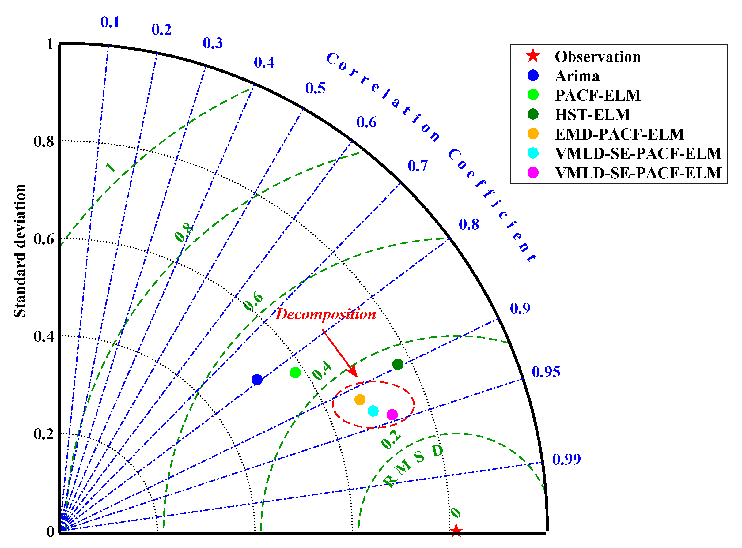
  A Taylor diagram can provide a visual framework for comparing the prediction results of a model to a reference model. It can represent the relevant information of various prediction models in a centralized way, which fully and clearly reflects the prediction capabilities of different models. Taylor diagrams have been widely adopted in recent years as an effective method for assessing the predictive ability of different models.

4. Case Study

4.1. Description of the Dam Project and Datasets

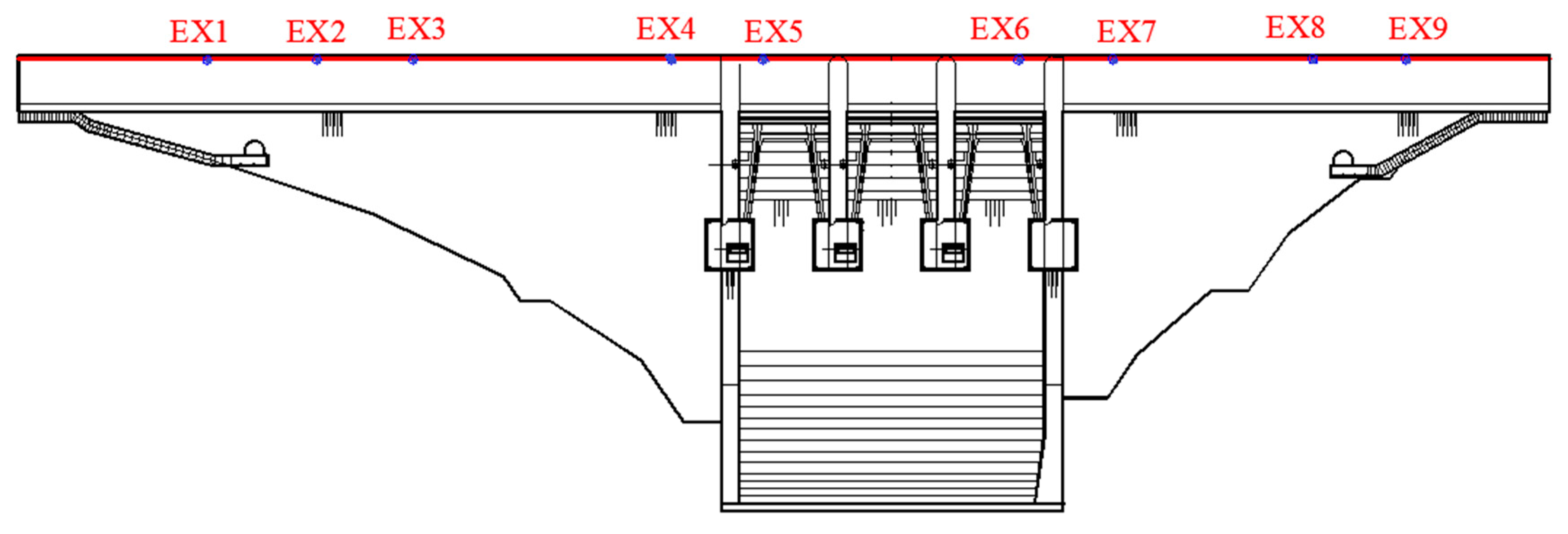
A Roller Compacted Concrete (RCC) gravity dam is located in southeast China. The dam crest elevation is at 634.40 m and the maximum height of the dam is 72.40 m. The length and width of the dam crest are 206.00 and 7.50 m, respectively. The upstream face of the dam body is vertical, and the downstream face of the retaining dam section has a dam slope of 1:0.72. The overflow dam section is located in the middle of the dam, and the weir crest elevation is at 621.00 m, with three overflow surface holes and three 12 × 12 m curved gates set (Figure 5).

This paper mainly studies the horizontal displacement of the top of the RCC gravity dam. A gravity dam has the characteristic of ensuring a stable state by the own gravity of the dam and cohesion with foundation. Therefore, dam failures are often the results of overtopping and penetration cracks in a section of the dam, which can be directly identified by the horizontal displacement. The displacement at the top of the dam is the most obvious and reflective of the deformation of the whole dam section, so the horizontal monitoring system of gravity dams is usually arranged at the top of the dam. Therefore, in this study, the horizontal displacement at the top of the dam is modeled and analyzed in order to verify the correctness of the proposed model.

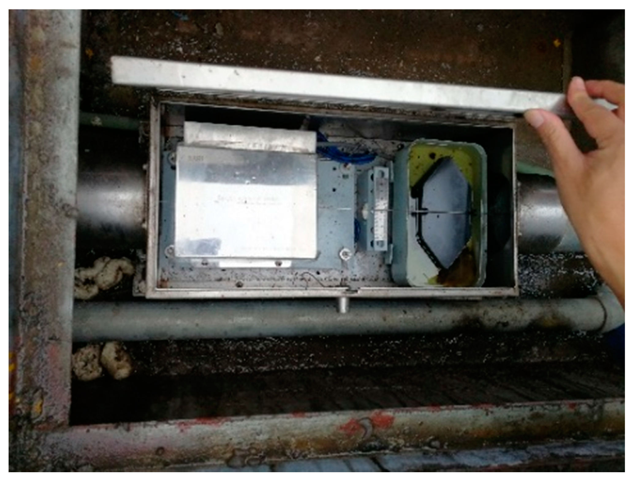
The horizontal displacement of the dam is measured by the tension wire alignment system, with one measurement point arranged in each dam section (Figure 5). The measurement point of the monitoring system is shown in Figure 6. For gravity dams, the middle dam section is generally the most important section of the dam and is often studied as a typical dam section, so the monitoring data related to horizontal displacements at the EX5 measurement point on the 4th dam section are selected for analysis (to the left bank is positive, to the right bank is negative).

For the horizontal displacement monitoring data at EX5, 739 daily observations from 6 June 2016 to 22 October 2018 were selected as the research object, and the missing values and outliers during this period were pre-processed. The monitoring data were divided into training set F (1st–709th measurements) and testing set T (710th–739th measurements). The processed data series is shown in Figure 7.

4.2. Data Decomposition

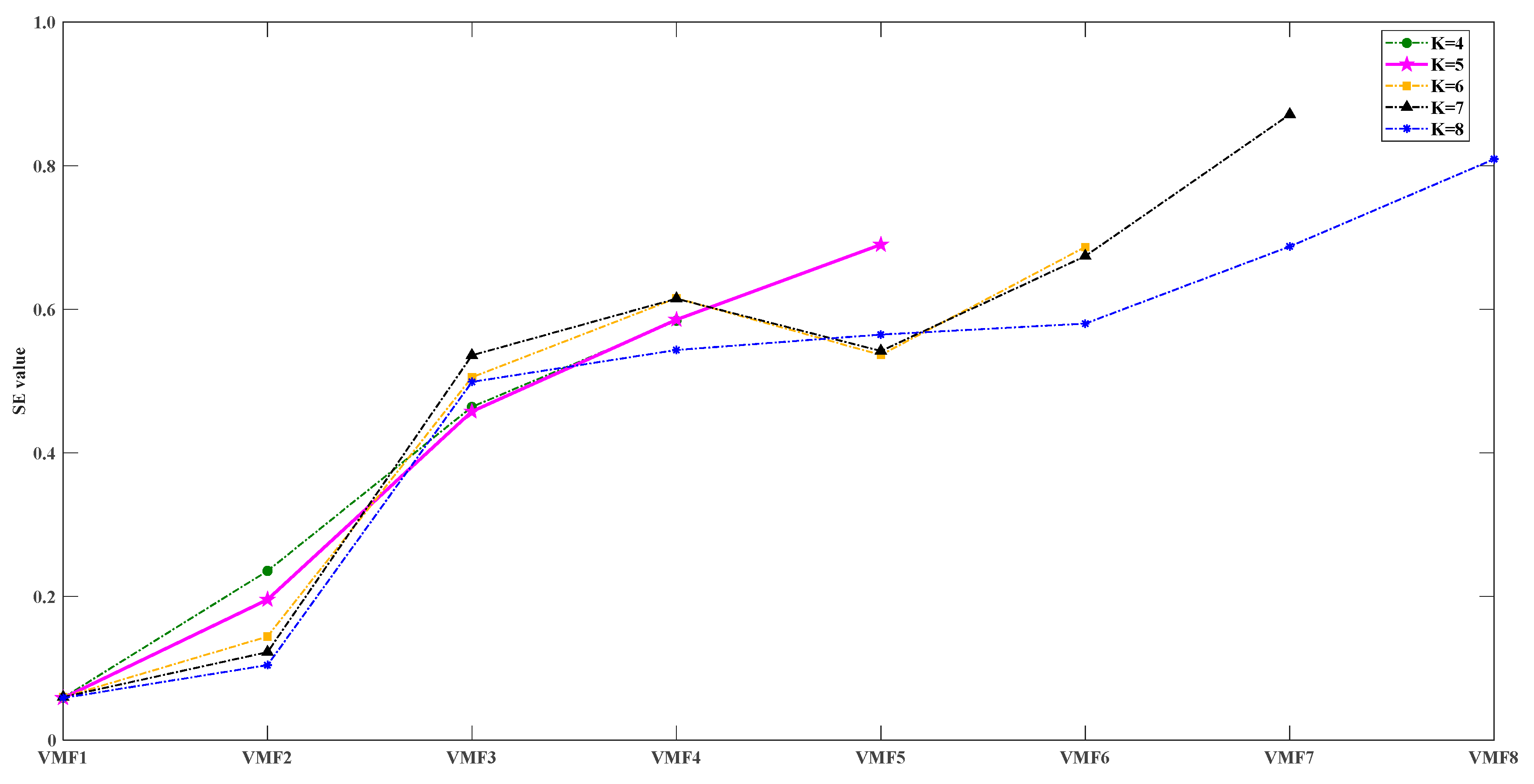
As can be seen in Figure 4, prior to VMD decomposition, the decomposition modulus should first be determined so that the characteristics of the original data can be fully extracted, which is essential for the application of VMD. We propose a new method for determining the optimal K value by the variation in the SE values of the subsequences. The SE values of VMF subsequences at different K values and their curves are shown in

Table 1. SE values of VMF subsequences at different K values.

K	SE Values
	VMF1	VMF2	VMF3	VMF4	VMF5	VMF6	VMF7	VMF8
4	0.0590	0.2356	0.4641	0.5840	/	/	/	/
5	0.0587	0.1958	0.4576	0.5857	0.6901	/	/	/
6	0.0598	0.1442	0.5054	0.6155	0.5364	0.6868	/	/
7	0.0600	0.1225	0.5359	0.6148	0.5419	0.6741	0.8714	/
8	0.0586	0.1044	0.4989	0.5433	0.5648	0.5801	0.6875	0.8092

and Figure 8, respectively.

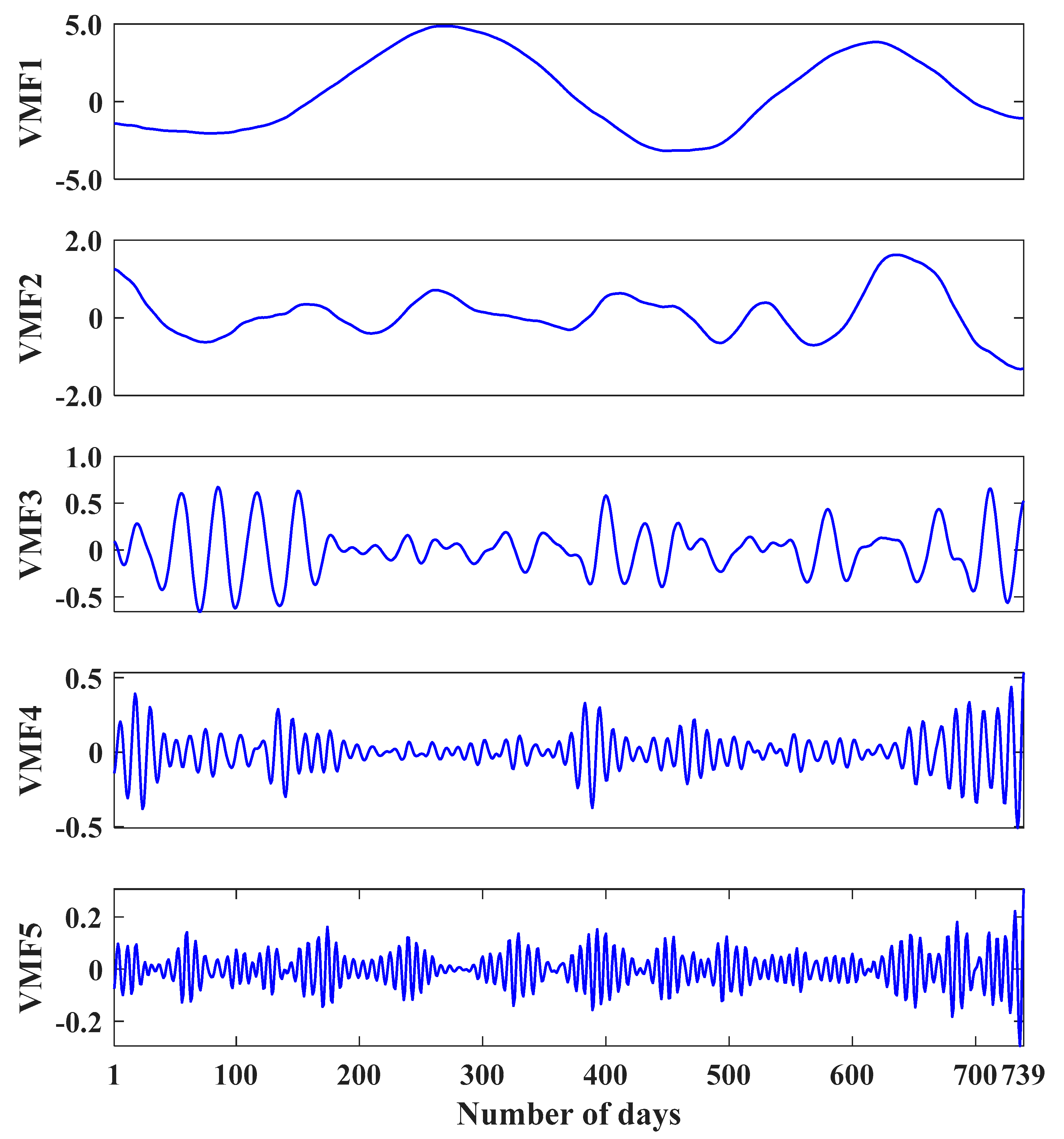
Obviously, when K = 5, the SE values for VMFs show a monotonically increasing trend and the difference between the SE values of the two subsequence is relatively large. When the K value increases to 6–8, it can be seen from Figure 5 that the SE curves corresponding to the above values (K = 6–8) have similar results at both VMF₃ and VMF₅ points, which will lead to modal confusion, implying that the VMD is over-decomposed. Meanwhile, the decomposition will be insufficient if the value of K decreases. Therefore, in this case, K = 5 is the best value for VMD decomposition, and the results are shown in Figure 9. The built-in parameters of the VMD algorithm are shown in

Table 2. Parameters of VMD algorithm used in our case.

Parameters	$\mathit{\alpha }$	$\mathit{\tau }$	$\mathit{K}$	$\mathit{D}\mathit{C}$	$\mathit{i}\mathit{n}\mathit{i}\mathit{t}$	$\mathit{t}\mathit{o}\mathit{l}$
Values	2000	0	5	0	1	1 × 10−7

.

4.3. Input Selection by PACF

After decomposing the DD sequence in the previous section to obtain the five VMFs, it is necessary to establish ELM prediction models for these five subsequences separately. Prior to this, input variables of ELMs should be determined with the PACF method according to Section 2.3. Figure 10 shows the corresponding PACF results for each VMF, and the best input variables for each VMF are shown in

Table 3. The input variables of each VMF.

Series	Numbers of Input	Input Variables
VMF1	5	$x_{t-1}~x_{t-5}$
VMF2	5	$x_{t-1}~x_{t-5}$
VMF3	9	$x_{t-1}~x_{t-9}$
VMF4	4	$x_{t-1}~x_{t-4}$
VMF5	6	$x_{t-1}~x_{t-6}$

.

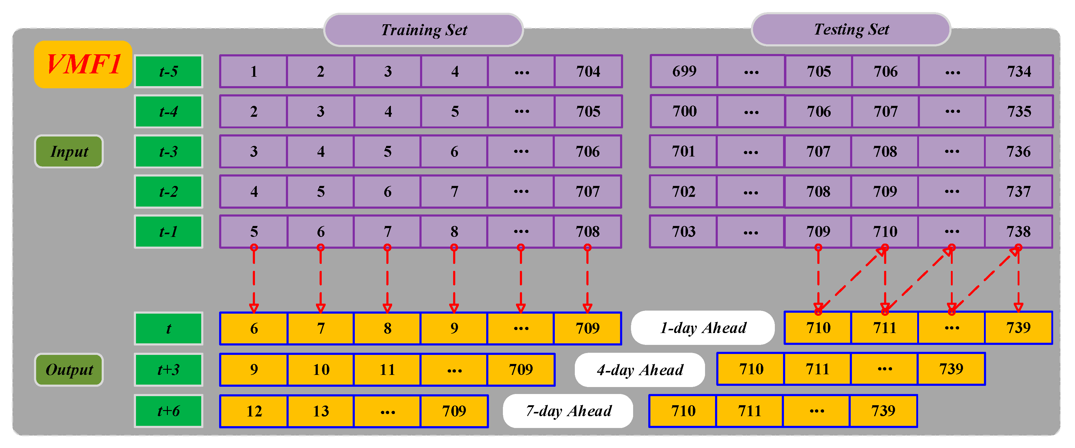
Take VMF1 as an example to illustrate how to select the input variables through the PACF results in Figure 10. For VMF₁, the PACF value falls at the 95% confidence interval when the lag is 6d, so the input variables corresponding to VMF₁ are the five values between (t − 5)d and (t − 1)d, and the output variable is the value of td. In order to guide the operation of the dam more comprehensively, the proposed model is also analyzed for different prediction periods (td, (t + 3)d and (t + 6)d) in this study. Taking VMF₁ as an example, the specific process of implementation is illustrated in Figure 11.

4.4. Determination of the ELM Structure Frameworks

After determining the input variables of the VMFs, we need to build an ELM-based, data-driven prediction model for each subsequence. Due to the stochastic nature of the ELM models, the ELM prediction results in this paper are based on the average of ten calculations with the removal of four outliers. During the prediction process, a corresponding ELM model is established for each subsequence, so that the number of the ELMs and the decomposition modulus are consistent. The output of each ELM represents the predicted results of the corresponding VMF, and the final prediction result is obtained by summing the predictions of all ELMs.

Since the prediction accuracy of ELMs will directly affect the prediction accuracy of the model, the selection of appropriate ELM parameters is crucial. The ELM model has two adjustable parameters, $g\left(x\right)$ and $l$, mentioned in Section 2.4. Sigmoid function is chosen as the $g\left(x\right)$ in this study. Meanwhile, the performance of an ELM model also depends on $l$, which can be obtained by Equation (24) as the ELM belongs to SLFNs.

$$l=round\left(\sqrt{n+m}+rand\left(1~10\right)\right)$$

(24)

In this study, $n$ and $m$ represent the number of input and output variables determined in Section 4.3, respectively. Since the original displacement sequence is decomposed into five VMFs, correspondingly, five ELM prediction models will be constructed. Equation (24) has given the method of determining the number of hidden layer neurons, and thus the structural framework of each ELM can be determined, expressed as ‘$n-l-m$’. Take VMF₁ as an example to illustrate the determination process of the ELM structural framework: the initial ELM structural framework of VMF1 is ‘5-$l$-1’. According to Equation (24), the best $l$ of the model is located at interval [3,12] or its neighboring values, and ten operations are performed for different hidden layer neurons to calculate each performance indicators. The results show that when $l=10$, the learning performance of the ELM is the best, so that the structure framework of the ELM model corresponding to VMF1 can be determined as ‘5-10-1’. The ELM structure frameworks of VMF2-VMF5 can be obtained by the same method, as shown in

Table 4. ELM structure framework of each VMF.

Prediction Model	$\mathit{n}-\mathit{l}-\mathit{m}$
ELMVMF1	5-10-1
ELMVMF2	5-12-1
ELMVMF3	9-15-1
ELMVMF4	4-10-1
ELMVMF5	6-12-1

.

4.5. Results and Discussion

4.5.1. Construction of the VMD-SE-PACF-ELM Model

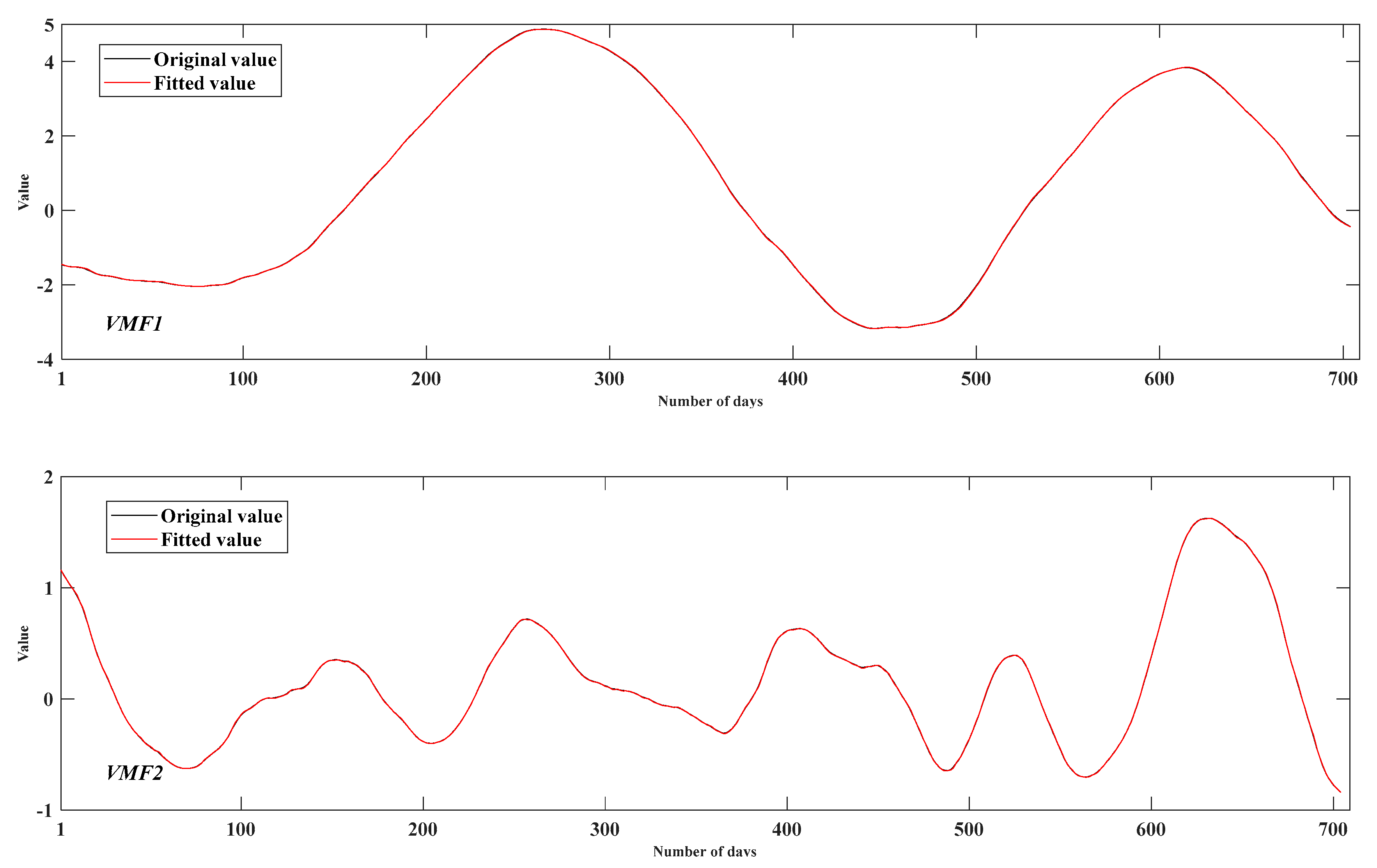
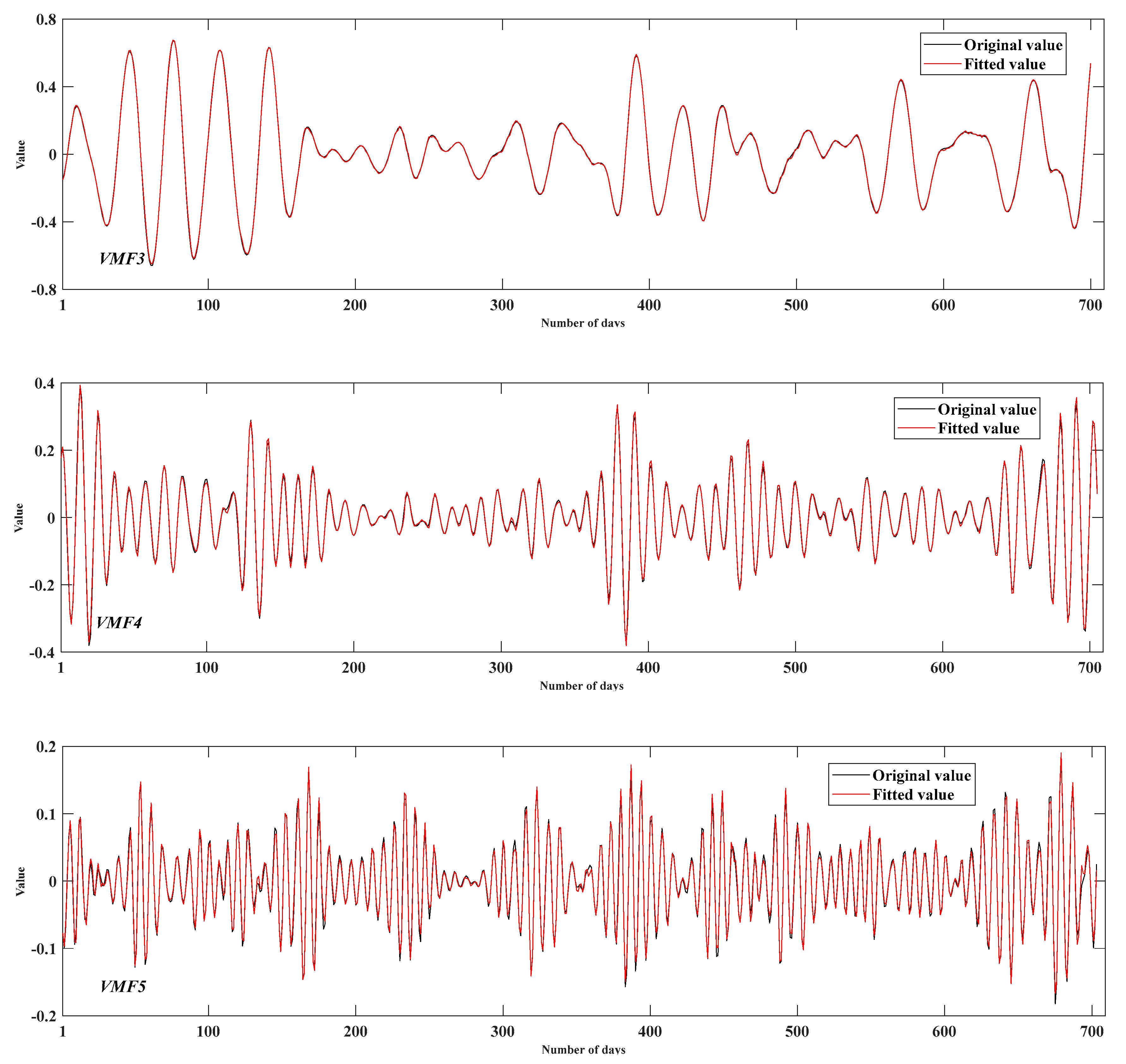
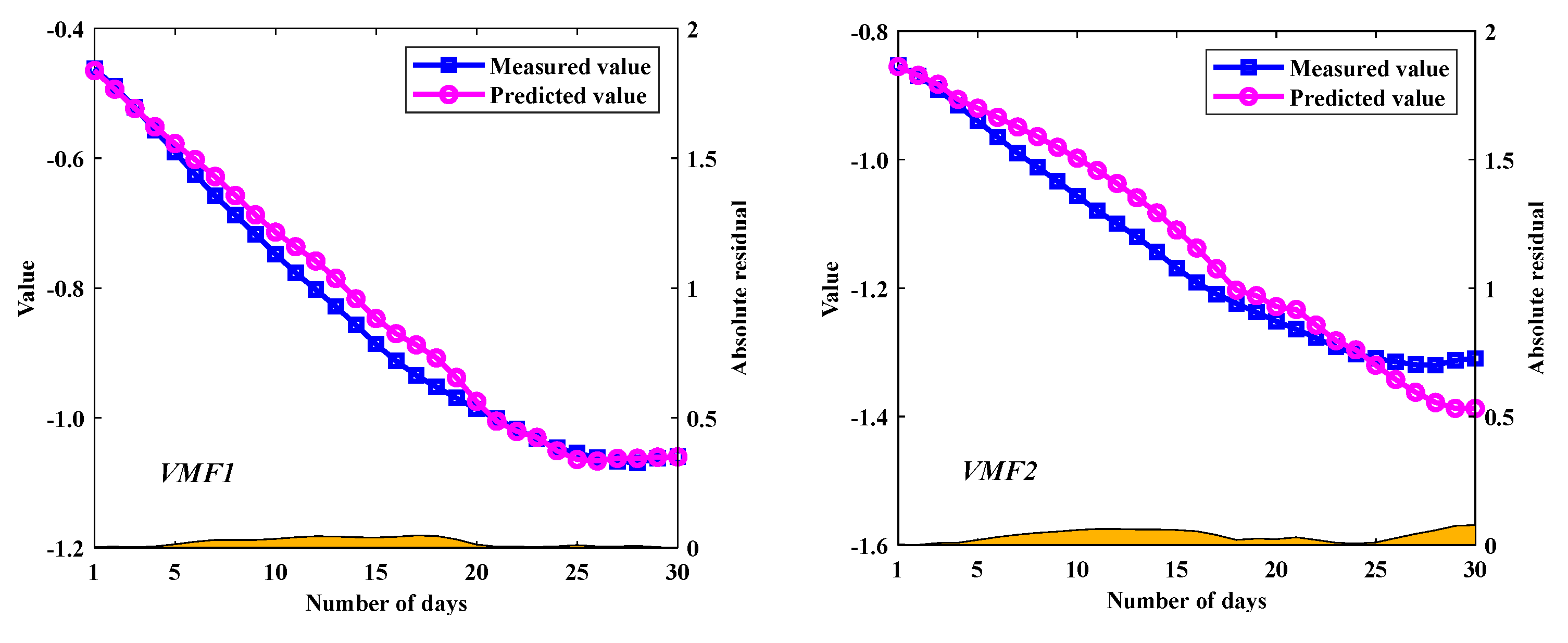
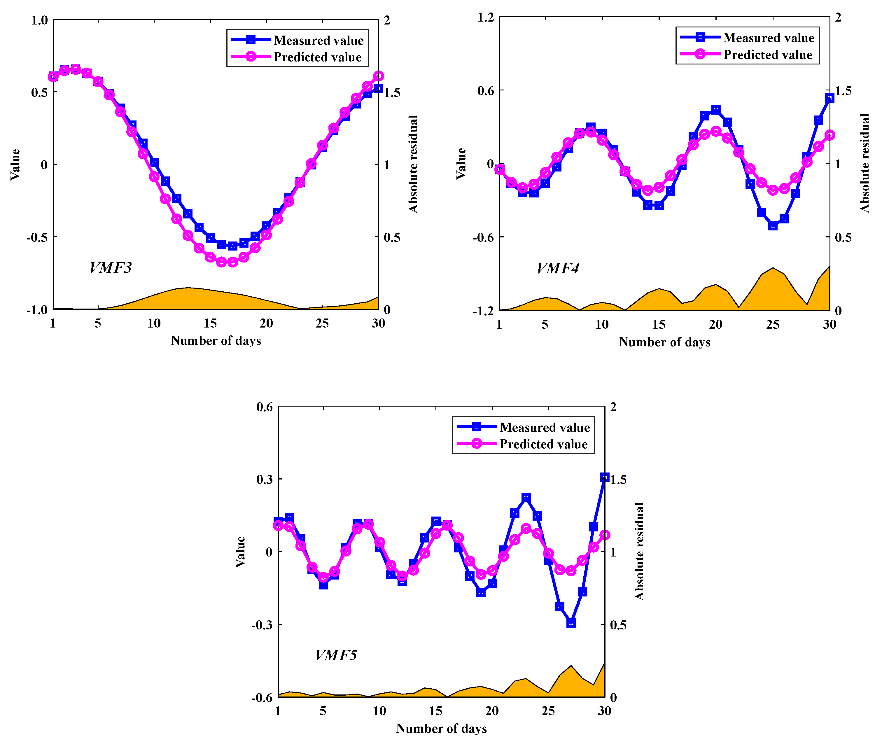
The ELM models with different structural frameworks are used to train and predict the VMF components separately, and then overlay the prediction results of each component to complete the construction of the VMD-SE-PACF-ELM model. During the prediction process, the result of each step are used to predict the next value until the 30th prediction result is obtained (Figure 11). The training and prediction results for each VMF are shown in Figure 12 and Figure 13, respectively. The yellow areas in Figure 13 represent the absolute residuals of the prediction results.

It can be seen from Figure 12 and Figure 13 that the VMF₁, VMF₂ and VMF₃ components have good fitting capability and low prediction error. In comparison, the fitting and prediction results for VMF4 and VMF5 are somewhat different from the actual values near the curve inflection points, but the overall results are consistent with the trend of the actual values. Therefore, it can be initially concluded that the use of the VMD algorithm can effectively decompose the DD fluctuation information, thereby improving the prediction performance of the model. Here we use RMSE, MAE and R² to quantify the performance of the training and testing phases of ELMs, as shown in

Table 5. Evaluation indicators of training and testing set for each sub-model.

Prediction Model	Training Set			Testing Set
	RMSE	MAE	R2	RMSE	MAE	R2
ELMVMF1	0.0014	0.0011	0.9998	0.0262	0.0201	0.9906
ELMVMF2	0.0015	0.0013	0.9980	0.0431	0.0366	0.9542
ELMVMF3	0.0026	0.0020	0.9989	0.0764	0.0580	0.9820
ELMVMF4	0.0047	0.0035	0.9972	0.1339	0.1034	0.9105
ELMVMF5	0.0056	0.0042	0.9841	0.0843	0.0603	0.7465
VMD-SE-PACF-ELM	/	/	/	0.2996	0.2343	0.8722

. Obviously, ELM_VMF1 has the smallest RMSE and MAE values and the largest R² value in the training and testing phases, followed by ELM_VMF2 and ELM_VMF3, and these three sub-models all show strong performance. ELM_VMF4 and ELM_VMF5 have relatively large errors during the training and testing phases, but their predictive accuracy is still at a high level so it does not affect the overall performance of the model.

To further illustrate the necessity of using the VMD decomposition algorithm in the prediction process of the ELM model, Figure 14 shows the prediction results and evaluation indicators before and after VMD optimization. In Figure 14, ‘VMD Optimized ELM’ represents the VMD-SE-PACF-ELM model, and ‘PACF-ELM’ represents the ELM model based on PACF to determine input variables. The left side of the figure is a bar graph of the performance evaluation indicators (RMSE, MAE and R²) of the two models, and the right side is the graph of the predicted results. Obviously, the deformation prediction result of the ELM model optimized based on the VMD algorithm has smaller RMSE and MAE as well as a larger R² compared to the single ELM model. Combined with the prediction curves, the following conclusions can be obtained: if the ELM model is used directly to predict the deformation time series with strong fluctuation characteristics, it is not possible to get accurate prediction results; however, the prediction results of the VMD-optimized ELM model are closer to the real values of the DD, which means that the VMD algorithm can decompose the original deformation series into several subsequences with good deformation characteristics. The prediction performance of the model will be greatly improved by modeling and predicting each subsequence.

4.5.2. Prediction Results Considering the ER

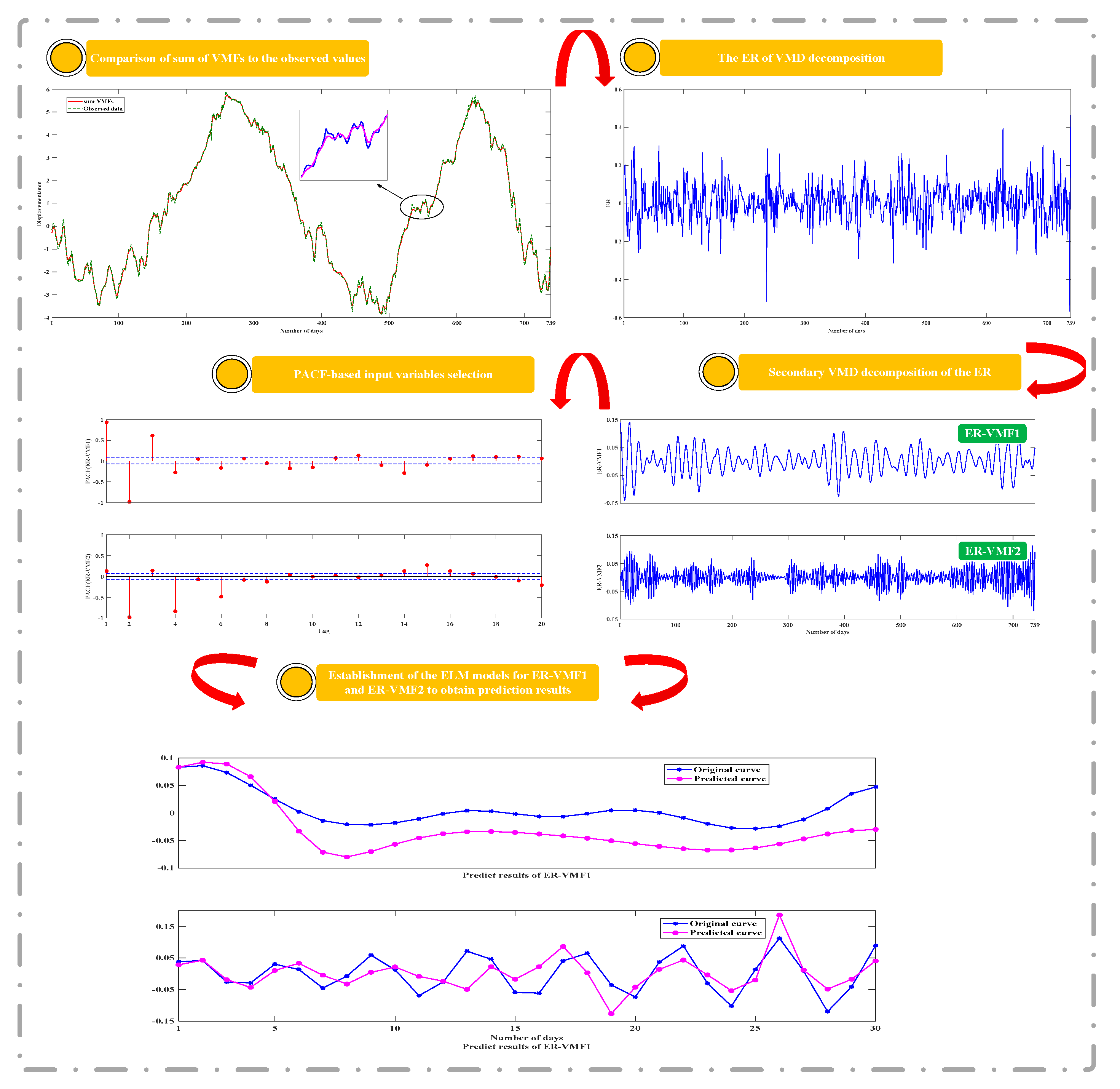
Although the VMD-SE-PACF-ELM model greatly improves the prediction performance, its prediction results fail to show the fluctuation characteristics of the DD well. Considering that the ER obtained after VMD decomposition contains some of the fluctuation characteristics of the original sequence, it is necessary to extract the sequence and to explore and analyze the deformation features embedded in it. Due to the strong nonlinearity and nonstationarity of the ER, direct modeling and prediction of it with the ELM model will lead to the prediction results being messy and impractical. Therefore, we propose to perform a secondary decomposition of the ER by the VMD algorithm to obtain subsequences with relatively stable deformation characteristics, which are recorded as ER-VMFs. Just like the original sequence, the decomposition modulus of the ER is first determined by the SE method. By analysis, the optimal decomposition modulus of ER is 2, and the obtained subsequences are denoted as ER-VMF₁ and ER-VMF₂. PACF analysis is then performed for each ER-VMF to determine the input variables for the prediction model. The specific analysis process of the ER is shown in Figure 15.

As can be seen in Figure 15, the VMD-decomposed ER is able to achieve better prediction results. The prediction results of the proposed model can be obtained by summing it up with the prediction results of the VMD-SE-PACF-ELM model. The prediction results and evaluation indicators of the models before and after considering ER are shown in Figure 16. The left side of the figure is a bar graph of the performance evaluation indicators (RMSE, MAE and R²), and the right side is a graph of the predicted results.

From Figure 16, the following conclusion can be drawn: the prediction results of the model without considering ER can reflect the overall trend of the time series, but cannot well capture the fluctuation characteristics of the original data. Through the analysis of ER, the prediction results of the hybrid model not only become more accurate, but also better reflect the fluctuation characteristics of the DD. Therefore, the analysis of ER has practical engineering significance.

4.5.3. Comparison with Other Benchmark Models

To further verify the superiority of the VMD-SE-ER-PACF-ELM model, its performance is compared with that of some benchmark models in this section. In addition to PACF-ELM and VMD-SE-PACF-ELM prediction models, three other DD prediction models, namely EMD-PACF-ELM, hydrostatic-seasonal-time (HST)-ELM and Arima models, are established. The EMD-PACF-ELM model can be used to verify that the VMD algorithm outperforms the EMD algorithm in DD prediction; the HST-ELM model can validate that the performance of the DD prediction model based on VMD decomposition is better than the ELM model based on statistical optimization, and the Arima model can demonstrate that the proposed model outperforms traditional time series prediction method in terms of prediction accuracy. The prediction results and performance evaluation indicators of each model are shown in Figure 17, where the bar graph of the performance evaluation indicators of each model is shown on the left and the curve of the prediction results is shown on the right.

As can be seen in Figure 17, both the evaluation indicators and the prediction curves show that Arima has the worst performance. In contrast to Arima, the prediction performance of the HST-ELM model is significantly better. Another important conclusion of Figure 17 is that the prediction results of the models combined with the signal decomposition methods (EMD, VMD) always outperform the other models. Meanwhile, the VMD-SE-ER-PACF-ELM model outperforms the EMD-PACF-ELM model, which indicates that the VMD algorithm used in this study to pre-process the deformation sequence is better than the EMD algorithm. Bar and curve graphs can provide a visual assessment of the prediction ability of the models and the correspondence between the observations and the model predictions. However, performance evaluation indicators can more accurately quantify the predicted performance of each model.

Table 6. Evaluation indicators of different prediction models.

	RMSE	MAE	R2
Arima	0.5955	0.4320	0.6259
PACF-ELM	0.5630	0.4085	0.6888
HST-ELM	0.4400	0.2862	0.8047
EMD-PACF-ELM	0.3341	0.2686	0.8398
VMD-SE-PACF-ELM	0.2996	0.2343	0.8722
VMD-SE-ER-PACF-ELM	0.2755	0.2087	0.8912

shows the performance evaluation indicators for the six models including PACF-ELM and VMD-SE-PACF-ELM.

The RMSE values of each model are: 0.2755 (VMD-SE-ER-PACF-ELM), 0.2996 (VMD-SE-PACF-ELM), 0.3341 (EMD-PACF-ELM), 0.4400 (HST-ELM), 0.5630 (PACF-ELM) and 0.5955 (Arima). Compared to other models, the RMSEs of the VMD-SE-ER-PACF-ELM model are reduced by 8.04%, 17.54%, 37.39%, 51.07% and 53.74%, respectively. Meanwhile, the values of MAE are: 0.2087 (VMD-SE-ER-PACF-ELM), 0.2343 (VMD-SE-PACF-ELM), 0.2686 (EMD-PACF-ELM), 0.2862 (HST-ELM), 0.4085 (PACF-ELM) and 0.4320 (Arima). The MAE values of the proposed model are reduced by 10.93%, 22.30%, 27.08%, 48.91% and 51.69%, respectively, compared to other models. The above results are consistent with the relatively high R² values (0.8912 for the VMD-SE-ER-PACF-ELM, 0.8722 for the VMD-SE-PACF-ELM, 0.8398 for the EMD-PACF-ELM, 0.8047 for the HST-ELM, 0.6888 for the PACF-ELM and 0.6259 for the Arima model). Compared to other models, the R² value of the proposed model in this paper has increased by 2.18%, 6.12%, 10.75%, 29.38% and 42.39%, respectively. Through calculation and comparison of the performance evaluation indicators of various models, we find that the VMD-SE-ER-PACF-ELM model is superior to all the other models in the performance of DD prediction.

Furthermore, Figure 18 shows the Taylor diagram of the prediction performance of each model. It is clear that Arima has the worst prediction performance and HST-ELM outperforms the traditional time series prediction method. In addition, the prediction performance of the ELM model optimized based on the decomposition algorithm is generally better than that of the model not optimized by this method, which indicates that the use of the decomposition algorithm to pre-process original sequences is an efficient method to optimize the prediction of DD. Among the different decomposition algorithms, VMD outperforms EMD and the consideration of the ER enables prediction results closer to the true values, which are consistent with the conclusions in Figure 17 and Table 6.

4.5.4. Performance of Different Prediction Periods Based on the Proposed Model

In summary, the proposed model has the smallest RMSE and MAE values and the largest R² value, and the prediction performance of the model is satisfactory. However, in the DD prediction, in addition to the prediction accuracy, the length of prediction period is also important to guide the normal and stable operation of a dam. In this section, we mainly discuss the influence of different prediction periods (1-, 4- and 7-day ahead) on the prediction performance of the proposed model. The specific implementation process for different periods is shown in Figure 11. The prediction results and performance evaluation indicators for each period are shown in Figure 19, where the bar graph of performance evaluation indicators for each model is shown on the left and the curves of prediction results is shown on the right. It is clear from Figure 19 that the VMD-SE-ER-PACF-ELM model is the most effective when the prediction period is one day, followed by the next best when the prediction period is four days, and the worst when the prediction period is seven days.

To further compare the impact of prediction periods on the results,

Table 7. Evaluation indicators of different prediction periods.

	RMSE	MAE	R2
1-day ahead	0.2755	0.2087	0.8912
4-day ahead	0.4198	0.3140	0.8130
7-day ahead	0.4547	0.3063	0.7047

presents the performance evaluation indicators of the predicted results for the corresponding periods. Their RMSE values are: 0.2755 (1d), 0.4198 (4d) and 0.4547 (7d). The RMSE values of one-day prediction period are reduced by 34.37% and 39.41%, respectively, compared to the other two periods. Meanwhile, the values of MAE are: 0.2087 (1d), 0.3140 (4d) and 0.3063 (7d). The MAE values of one-day prediction period are reduced by 33.54% and 31.86%, respectively, compared to the other two periods. The above results are consistent with the relatively high R² values (0.8912 for 1d, 0.8130 for 4d, and 0.7047 for 7d). Compared to other two periods, the R² value of one-day prediction period has increased by 9.62% and 26.47%, respectively. By calculating and comparing the performance evaluation indicators for each projection period, it can be concluded that the longer the prediction period, the worse the overall prediction performance of the model.

In addition, Figure 20 shows the Taylor diagram of prediction performance for different periods. Obviously, the model has the best prediction performance when the period is one day. When the period is seven days, the prediction result is the farthest from the true value and the performance is the worst. They are consistent with the conclusions drawn in Figure 19 and Table 7. Therefore, when using the VMD-SE-ER-PACF-ELM model to predict the DD in actual projects, the prediction period should be shortened as much as possible in order to obtain higher prediction performance.

5. Conclusions

In order to improve the prediction performance of nonstationary DD, a novel hybrid model based on the decomposition-composition framework is proposed, namely VMD-SE-ER-PACF-ELM. The details are as follows: (1) The VMD algorithm is used to decompose an original deformation sequence into a number of subsequences with good characteristics to improve the prediction performance. (2) The SE method is used to quantify the complexity of each subsequence in order to select the appropriate decomposition modulus. (3) The secondary VMD decomposition of the ER enables the prediction value to be closer to the actual deformation characteristics. (4) The PACF method is used to analyze the characteristics of each subsequence to extract the input variables. (5) The ELM models are used to predict the subsequences and their combination is the final prediction result. Meanwhile, the prediction performance of the VMD-SE-ER-PACF-ELM model is compared with those of Arima, PACF-ELM, HST-ELM, VMD-PACF-ELM, and VMD-SE-PACF-ELM models with RMSE, MAE, R², and Taylor diagrams as performance evaluation indicators.

The results show that the proposed VMD-SE-ER-PACF-ELM model has the best prediction performance among all prediction models. It can effectively predict nonstationary and nonlinear time series and significantly improve the prediction accuracy. In addition, we have also analyzed its performance under different prediction periods. The results show that the length of the prediction period is inversely proportional to the prediction accuracy, which can provide a priori knowledge for the normal operation and early warning of the dam projects.

Although the proposed method has good prediction results, there are still certain prediction errors. In this paper, the uncontrolled errors due to the randomness of the ELM model is the main cause of the prediction errors, which needs to be addressed in our future research. In addition, the idea of spatial relationships between the measurement points [51] will be introduced into the prediction to analyze the overall deformation effect of dams.

References

1. Su, H.Z.; Li, X.; Yang, B.B.; Wen, Z.P. Wavelet support vector machine-based prediction model of dam deformation. Mech. Syst. Signal. Process. 2018, 110, 412–427. [Google Scholar] [CrossRef]
2. Shao, C.F.; Gu, C.S.; Yang, M.; Xu, Y.X.; Su, H.Z. A novel model of dam displacement based on panel data. Struct. Contr. Health Monit. 2018, 25, e2037. [Google Scholar] [CrossRef]
3. Li, Y.T.; Bao, T.F.; Gong, J.; Shu, X.S.; Zhang, K. The Prediction of Dam Displacement Time Series Using STL, Extra-Trees, and Stacked LSTM Neural Network. IEEE Access 2020, 8, 94440–94452. [Google Scholar] [CrossRef]
4. Zhong, D.H.; Sun, Y.F.; Li, M.C. Dam break threshold value and risk probability assessment for an earth dam. Nat. Hazards 2011, 59, 129–147. [Google Scholar] [CrossRef]
5. Chen, S.Y.; Gu, C.S.; Lin, C.N.; Zhang, K.; Zhu, Y.T. Multi-kernel optimized relevance vector machine for probabilistic prediction of concrete dam displacement. Eng. Comput. Ger. 2020, 1–17. [Google Scholar] [CrossRef]
6. Salazar, F.; Morán, R.; Toledo, M.A.; Oñate, E. Data-based models for the prediction of dam behavior: A review and some methodological considerations. Arch. Comput. Method E 2017, 24, 1–21. [Google Scholar] [CrossRef] [Green Version]
7. Wu, Z.R. Safety Monitoring Theory and Its Application of Hydraulic Structures; Higher Education: Beijing, China, 2003. [Google Scholar]
8. Shi, Y.Q.; Yang, J.J.; Wu, J.L.; He, J.P. A statistical model of deformation during the construction of a concrete face rock-fill dam. Struct. Contr. Health Monit. 2018, 25, e2074. [Google Scholar] [CrossRef]
9. Gu, C.S.; Wu, Z.R. Safety Monitoring of Dams and Dam Foundations-Theories and Method and Their Application; Hohai University Press: Nanjing, China, 2006. [Google Scholar]
10. Kang, F.; Li, J.J.; Dai, J.H. Prediction of long-term temperature effect in structural health monitoring of concrete dams using support vector machines with Jaya optimizer and salp swarm algorithms. Adv. Eng. Softw. 2019, 131, 60–76. [Google Scholar] [CrossRef]
11. Kao, C.Y.; Loh, C.H. Monitoring of long-term static deformation data of Fei-Tsui arch dam using artificial neural network-based approaches. Struct. Contr. Health Monit. 2013, 20, 282–303. [Google Scholar] [CrossRef]
12. Bui, K.-T.T.; Tien, B.D.; Zhou, J.; Van Doan, C.; Revhaug, I. A novel hybrid artificial intelligent approach based on neural fuzzy inference model and particle swarm optimization for horizontal displacement modeling of hydropower dam. Neural Comput. Appl. 2018, 29, 1495–1506. [Google Scholar] [CrossRef]
13. Dai, B.; Gu, C.S.; Zhao, E.F.; Qin, X.N. Statistical model optimized random forest regression model for concrete dam deformation monitoring. Struct. Contr. Health Monit. 2018, 25, e2170. [Google Scholar] [CrossRef]
14. Salazar, F.; Toledo, M.A.; Oñate, E.; Morán, R. An empirical comparison of machine learning techniques for dam behaviour modelling. Struct. Saf. 2015, 56, 9–17. [Google Scholar] [CrossRef] [Green Version]
15. Mata, J.; De Castro, A.T.; Da Costa, J.S. Constructing statistical models for arch dam deformation. Struct. Contr. Health Monit. 2014, 21, 423–437. [Google Scholar] [CrossRef] [Green Version]
16. Li, D.Y.; Zhou, Y.C.; Gan, X.Q. Research on multiple points deterministic displacement monitoring model of concrete arch dam. J. Hydraul. Eng. 2011, 42, 981–985. [Google Scholar] [CrossRef]
17. Xi, G.Y.; Yue, J.P.; Zhou, B.X.; Tang, P. Application of an artificial immune algorithm on a statistical model of dam displacement. Comput. Math. Appl. 2011, 62, 3980–3986. [Google Scholar] [CrossRef] [Green Version]
18. RaziAnisheh, S.; Mahmoud Anisheh, S.; Jiryaei Sharahi, M.; Bastam, M. Application of finite difference method and pso algorithm in seismic analysis of narmab earth dam. Int. J. Comput. Appl. 2012, 54, 1–5. [Google Scholar] [CrossRef]
19. Torabi, S.; Yonesi, H.A.; Shahinejad, B. Calibration the area-reduction method in sediment distribution of Ekbatan reservoir dam using genetic algorithms. Model. Earth Syst. Environ. 2015, 1, 21. [Google Scholar] [CrossRef] [Green Version]
20. Moody, J.; Darken, C. Fast Learning in Networks of Locally-Tuned Processing Units. Neural Comput. 1989, 1, 281–294. [Google Scholar] [CrossRef]
21. Vapnik, V.; Golowich, S.E.; Smola, A. Support vector method for function approximation, regression estimation, and signal processing. Adv. Neural Inf. Process. Syst. 1996, 9, 281–287. [Google Scholar]
22. Huang, G.B.; Zhu, Q.Y.; Siew, C.K. Extreme learning machine: Theory and applications. Neurocomputing 2006, 70, 489–501. [Google Scholar] [CrossRef]
23. Huang, G.B.; Chen, L.; Siew, C.K. Universal approximation using incremental constructive feedforward networks with random hidden nodes. IEEE Press. 2006, 17, 879–892. [Google Scholar] [CrossRef] [PubMed] [Green Version]
24. Huang, G.B.; Chen, L. Convex incremental extreme learning machine. Neurocomputing 2007, 70, 3056–3062. [Google Scholar] [CrossRef]
25. Shamshirband, S.; Mohammadi, K.; Chen, H.L.; Samy, G.N.; Petković, D.; Ma, C. Daily global solar radiation prediction from air temperatures using kernel extreme learning machine: A case study for Iran. J. Atmos. Sol. Terr. Phys. 2015, 134, 109–117. [Google Scholar] [CrossRef]
26. Shamshirband, S.; Mohammadi, K.; Lee, P.L.; Petkovic, D.; Mostafaeipour, A. A comparative evaluation for identifying the suitability of extreme learning machine to predict horizontal global solar radiation. Renew. Sustain. Energy Rev. 2015, 52, 1031–1042. [Google Scholar] [CrossRef]
27. Huang, Y.W.; Lai, D.H. Hidden node optimization for extreme learning machine. Aasri Procedia 2012, 3, 375–380. [Google Scholar] [CrossRef]
28. Su, H.Z.; Wu, Z.R.; Wen, Z.P. Identification model for dam behavior based on wavelet network. Comput. Aided Civ. Infrastruct. Eng. 2007, 22, 438–448. [Google Scholar] [CrossRef]
29. Napolitano, G.; Serinaldi, G.; See, L. Impact of EMD decomposition and random initialisation of weights in ANN hindcasting of daily stream flow series: An empirical examination. J. Hydrol. 2011, 406, 199–214. [Google Scholar] [CrossRef]
30. Duan, W.Y.; Han, Y.; Huang, L.M.; Zhao, B.B.; Wang, M.H. A hybrid EMD-SVR model for the short-term prediction of significant wave height. Ocean Eng. 2016, 124, 54–73. [Google Scholar] [CrossRef]
31. Wang, J.; Tang, L.Y.; Luo, Y.Y.; Ge, P. A weighted EMD-based prediction model based on TOPSIS and feed forward neural network for noised time series. Knowl. Based Syst. 2017, 132, 167–178. [Google Scholar] [CrossRef]
32. Dragomiretskiy, K.; Zosso, D. Variational mode decomposition. IEEE Trans. Signal. Process. 2014, 62, 531–544. [Google Scholar] [CrossRef]
33. Feng, Z.K.; Niu, W.J.; Tang, Z.Y.; Jiang, Z.P.; Xu, Y.; Liu, Y.; Zhang, H.R. Monthly runoff time series prediction by variational mode decomposition and support vector machine based on quantum-behaved particle swarm optimization. J. Hydrol. 2020, 583, 124627. [Google Scholar] [CrossRef]
34. Niu, W.J.; Feng, Z.K.; Chen, Y.B.; Zhang, H.R.; Cheng, C.T. Annual streamflow time series prediction using extreme learning machine based on gravitational search algorithm and variational mode decomposition. J. Hydrol. Eng. 2020, 25, 04020008. [Google Scholar] [CrossRef]
35. Seo, Y.; Kim, S.; Singh, V.P. Machine Learning Models Coupled with Variational Mode Decomposition: A New Approach for Modeling Daily Rainfall-Runoff. Atmosphere 2018, 9, 251. [Google Scholar] [CrossRef] [Green Version]
36. Naik, J.; Bisoi, R.; Dash, P.K. Prediction interval forecasting of wind speed and wind power using modes decomposition based low rank multi-kernel ridge regression. Renew. Energy 2018, 129, 357–383. [Google Scholar] [CrossRef]
37. Abdoos, A.A. A new intelligent method based on combination of VMD and ELM for short term wind power forecasting. Neurocomputing 2016, 203, 111–120. [Google Scholar] [CrossRef]
38. Zhang, D.; Peng, X.; Pan, K. A novel wind speed forecasting based on hybrid decomposition and online sequential outlier robust extreme learning machine. Energy Convers. Manag. 2019, 180, 338–357. [Google Scholar] [CrossRef]
39. Xu, C.; Chen, H.; Xun, W.; Zhou, Z.; Liu, T.; Zeng, Y.; Ahmad, T. Modal decomposition based ensemble learning for ground source heat pump systems load forecasting. Energy Build. 2019, 194, 62–74. [Google Scholar] [CrossRef]
40. Sun, W.; Huang, C.C. A carbon price prediction model based on secondary decomposition algorithm and optimized back propagation neural network. J. Clean. Prod. 2019, 243, 118671. [Google Scholar] [CrossRef]
41. Xie, T.; Zhang, G.; Hou, J.; Xie, J.; Lv, M.; Liu, F. Hybrid forecasting model for non-stationary daily runoff series: A case study in the Han River Basin, China. J. Hydrol. 2019, 577, 123915. [Google Scholar] [CrossRef]
42. Niu, M.F.; Hu, Y.Y.; Sun, S.L.; Liu, Y. A novel hybrid decomposition-ensemble model based on VMD and HGWO for container throughput forecasting. Appl. Math. Model. 2018, 57, 163–178. [Google Scholar] [CrossRef]
43. Wu, Q.L.; Lin, H.X. Daily urban air quality index forecasting based on variational mode decomposition, sample entropy and LSTM neural network. Sustain. Cities Soc. 2019, 50, 101657. [Google Scholar] [CrossRef]
44. Zhang, Y.G.; Pan, G.F.; Chen, B.; Han, J.Y.; Zhao, Y.; Zhang, C.H. Short-term wind speed prediction model based on GA-ANN improved by VMD. Renew. Energy 2020, 156, 1373–1388. [Google Scholar] [CrossRef]
45. Zan, T.; Pang, Z.L.; Wang, M.; Gao, X.S. Research on Early Fault Diagnosis of Rolling Bearing Based on VMD. In Proceedings of the 2018 6th International Conference on Mechanical, Automotive and Materials Engineering (CMAME), Hong Kong, China, 10–12 August 2018. [Google Scholar] [CrossRef]
46. Zhou, J.; Xiang, B.P.; Ni, L.; AI, P.H. Research on Optimal Wavelet Packet Threshold Estimation Denoising Algorithm Based on Sample Entropy. Mach. Des. Res. 2018, 34, 39–42. [Google Scholar]
47. Zhang, Y.G.; Zhao, Y.; Kong, C.H.; Chen, B. A new prediction method based on VMD-PRBF-ARMA-E model considering wind speed characteristic. Energy Convers. Manag. 2020, 203, 112254. [Google Scholar] [CrossRef]
48. Richman, J.S.; Moorman, J.R. Physiological time-series analysis using approximate entropy and sample entropy. Ame. J. Physiol. Heart Circ. Physiol. 2000, 278, 2039–2049. [Google Scholar] [CrossRef] [PubMed] [Green Version]
49. Hao, Y.; Zhen, D.; Anbo, M. Ultra Short-Term Wind Power Forecasting Based on VMD-SE-IPSO-BNN. Electr. Meas. Instrum. 2018, 2, 8. [Google Scholar]
50. Sun, G.; Chen, T.; Wei, Z.; Sun, Y.; Zang, H.; Chen, S. A carbon price forecasting model based on variational mode decomposition and spiking neural networks. Energies 2016, 9, 54. [Google Scholar] [CrossRef] [Green Version]
51. Gu, C.S.; Fu, X.; Shao, C.F.; Shi, Z.W.; Su, H.Z. Application of spatiotemporal hybrid model of deformation in safety monitoring of high arch dams: A case study. Int. J. Environ. Res. Public Health 2020, 17, 319. [Google Scholar] [CrossRef] [Green Version]
Figure 1. Specific procedures of variational mode decomposition (VMD).
Applsci 10 05700 g001
Figure 2. Specific process of sample entropy (SE).
Applsci 10 05700 g002
Figure 3. Extreme learning machine (ELM) structure.
Applsci 10 05700 g003
Figure 4. Flow chart of dam deformation model based on VMD-SE-ER-PACF-ELM.
Applsci 10 05700 g004
Figure 5. Layout of wire alignment device observing horizontal displacements.
Applsci 10 05700 g005
Figure 6. Layout of tension wire alignment device observing horizontal displacements.
Applsci 10 05700 g006
Figure 7. Horizontal displacements at EX5 from 6th June 2016 to 22nd October 2018.
Applsci 10 05700 g007
Figure 8. Curves of SE values of VMF subsequences with different K values.
Applsci 10 05700 g008
Figure 9. Decomposition results by VMD.
Applsci 10 05700 g009
Figure 10. The PACF results of VMFs.
Applsci 10 05700 g010
Figure 11. The process of determining the input and output variables for VMF1.
Applsci 10 05700 g011
Figure 12. Training results for each VMF.
Applsci 10 05700 g012aApplsci 10 05700 g012b
Figure 13. Prediction results for each VMF.
Applsci 10 05700 g013aApplsci 10 05700 g013b
Figure 14. Comparison of prediction results before and after VMD optimization.
Applsci 10 05700 g014
Figure 15. Analysis process of the ER.
Applsci 10 05700 g015
Figure 16. Comparison of predicted results before and after considering ER.
Applsci 10 05700 g016
Figure 17. Comparison of prediction results via different models.
Applsci 10 05700 g017
Figure 18. Taylor diagram of the prediction performance of each model. * Blue contours represent Pearson correlation coefficient; black contours represent standard deviation of the simulated pattern; and green contours represent centered RMS error in the simulated field.
Applsci 10 05700 g018
Figure 19. Comparison of prediction results for different periods.
Applsci 10 05700 g019
Figure 20. Taylor diagram of prediction performance for different periods. * Blue contours represent Pearson correlation coefficient; black contours represent standard deviation of the simulated pattern; and green contours represent centered RMS error in the simulated field.
Applsci 10 05700 g020