Article

Bayesian Updating of Soil–Water Character Curve Parameters Based on the Monitor Data of a Large-Scale Landslide Model Experiment

1
College of Hydraulic and Environment Engineering, China Three Gorges University, Yichang 443002, China
2
Institute for Risk and Reliability, Leibniz University Hannover, Callinstr. 34, 30167 Hannover, Germany
3
Institute for Risk and Uncertainty, University of Liverpool, Peach Street, Liverpool L69 7ZF, UK
4
International Joint Research Center for Engineering Reliability and Stochastic Mechanics, Tongji University, Shanghai 200092, China
*
Authors to whom correspondence should be addressed.
Appl. Sci. 2020, 10(16), 5526; https://doi.org/10.3390/app10165526
Submission received: 30 June 2020 / Revised: 4 August 2020 / Accepted: 6 August 2020 / Published: 10 August 2020
(This article belongs to the Special Issue Novel Approaches in Landslide Monitoring and Data Analysis)

Abstract

:
It is important to determine the soil–water characteristic curve (SWCC) for analyzing landslide seepage under varying hydrodynamic conditions. However, the SWCC exhibits high uncertainty due to the variability inherent in soil. To this end, a Bayesian updating framework based on the experimental data was developed to investigate the uncertainty of the SWCC parameters in this study. The objectives of this research were to quantify the uncertainty embedded within the SWCC and determine the critical factors affecting an unsaturated soil landslide under hydrodynamic conditions. For this purpose, a large-scale landslide experiment was conducted, and the monitored water content data were collected. Steady-state seepage analysis was carried out using the finite element method (FEM) to simulate the slope behavior during water level change. In the proposed framework, the parameters of the SWCC model were treated as random variables and parameter uncertainties were evaluated using the Bayesian approach based on the Markov chain Monte Carlo (MCMC) method. Observed data from large-scale landslide experiments were used to calculate the posterior information of SWCC parameters. Then, 95% confidence intervals for the model parameters of the SWCC were derived. The results show that the Bayesian updating method is feasible for the monitoring of data of large-scale landslide model experiments. The establishment of an artificial neural network (ANN) surrogate model in the Bayesian updating process can greatly improve the efficiency of Bayesian model updating.

1. Introduction

The prediction of a landslide and its stability performance have always been key difficulties of engineering. Particularly for the sensitive and landslide-prone areas in reservoir areas or mountain areas, the water migration inside a landslide is very prominent for its stability [1,2,3]. The soil–water characteristic curve (SWCC) is the cornerstone of the seepage calculation of unsaturated soil. In the analysis of saturated-unsaturated seepage, it is very important to fully describe the function of the slope of the moisture content [4,5]. The preliminary prediction based on the survey data often deviates from the actual monitoring value. As the real conditions are very complicated, the mechanism cannot be fully grasped through analytical models. Therefore, the trial algorithm is often used to repeatedly correct the soil parameters to obtain results that match the monitoring value [6,7]. The Bayesian method provides an effective way to solve such problems. By using the detection data, a priori information, and model assumptions, the parameter update is realized and the parameter uncertainty is quantified [8,9]. This technique uses a set of output measurement data (such as a point in a multi-dimensional output space) [10,11]. The purpose of this paper is to solve the problem of how to check the parameters of a SWCC model of a landslide using the Bayesian updating method.
The SWCC is a crucial input for modeling the geotechnical problems with unsaturated soil. It can be describing the relationship between matric suction and volumetric water content in unsaturated soils [12]. The main feature of SWCC is that the slope of the residual water content or saturation function in the pore water pressure range is from negative to positive [13]. As a basic equation in unsaturated soil mechanics, it plays an important role in the application of unsaturated soil mechanics for studying the strengths, deformations, and permeabilities of soils [14]. Past studies have shown that the shear strength of unsaturated soils can be estimated by the SWCC [15,16,17]. It can be seen that these parameters play important roles in the safety of geotechnical engineering [18,19,20,21]. Therefore, the SWCC parameters are evaluated as a method to determine the unsaturated soil properties of landslides. In engineering practice, the SWCC is usually measured by field or laboratory tests. The typical methods used are: the tensiometer method, the pressure plate meter method, the cold mirror hygrometer method, and the filter paper method. The limited number of data points are then used to estimate the SWCC by best fitting them with some parametric SWCC models, such as the van Genuchten–Mualem model (VGM), the van Genuchten-Burdine model (VGB), the van Genuchten model (VG), and the Fredlund and Xing model (FX) [14,22].
This paper adopts the Bayesian updating method, which is essentially a Bayesian statistical reasoning problem [23], to study the uncertainty of the parameters involved in the model. The Bayesian method is a probabilistic method based on the application of Bayesian rules. The resulting solution is called the posterior distribution, which is a multi-dimensional probability distribution function in the update parameter space. The posterior distribution is usually a complex distribution, and in principle it is integral in the parameter space. It can be approximated by statistical methods and using modern algorithms, namely, the Markov chain Monte Carlo (MCMC) method [24]. The distribution model, also known as the maximum posterior probability (MAP), defines the updated model, and the distribution around the model provides a measure of confidence in the model. The peak distribution often means a high degree of confidence in the updated model, and shallowness may make uncertain the choice of parameters [25,26]. Bayesian updating and prediction methods are widely used in geotechnical engineering, such as pile bearing capacity analysis, soft soil consolidation inversion analysis, jack-up drilling platform bearing capacity analysis, foundation pit support under normal use protection, and excavation problems and slope stability problems [27]. The key difficulty of the Bayesian method lies in the calculation of the MAP distribution. Because of the complexity of the MAP distribution and the possibility of involving high-dimensional integration problems, the direct numerical integration method is less efficient. To overcome this problem, the MCMC method avoids the computational complexity of directly solving the MAP distribution by generating a large number of random samples that obey the MAP distribution, and then it uses these random samples to characterize the MAP distribution [28,29]. Metropolis–Hastings (M–H) algorithm, as one of the commonly used MCMC methods, has been widely used in geotechnical engineering [30]. In this paper, the M–H method is used to generate a large number of MCMC random samples that follow the MAP distribution parameters, such as the posterior mean, posterior standard deviation, and posterior distribution. These statistics are the basic inputs for reliability analysis of geotechnical engineering [31].
Therefore, the purpose of this article is to show how to use MCMC simulations to effectively describe SWCC parameter uncertainty involving random variables. The structure of this article is as follows. First, the theory of the SWCC and the Bayesian theory of parameter uncertainty are introduced. Second, the hybrid Markov chain with emphasis on the uncertainty characterization of the geotechnical model is introduced, and a framework for updating the posterior distribution of the parameters of SWCC is introduced. Then, a large-scale landslide model experiment is used to illustrate how to obtain the posterior distribution of the parameters of the SWCC through Bayesian updating. Finally, we analyze the influencing factors of posterior distribution and characterize the uncertainty of SWCC parameters.

2. Theories and Methods

2.1. Soil–Water Characteristic Curve

Among the existing empirical equations for curve-fitting of the SWCC, the most commonly used VG model was adopted in the present study, which is given by [12]:
θ w = θ r + θ s θ r [ 1 + λ a n ] 1 1 n
where θ w is the volumetric water content; θ r is the residual volumetric water content; θ s is the saturated volumetric water content; λ is matric suction; a and n are non-negative curve fitting parameters.
To obtain the prior distribution of SWCC parameters, a simple sensitivity analysis of the modeling parameters sheds light on the possible range of the numeric values of the parameters [23]. The morphology of the SWCC between a from 0.1 to 10 and n from 1.1 to 5 was studied. Figure 1a describes the influence of the value of a on the SWCC model when n is 5. Figure 1b describes the effect of the value of n on the SWCC model when a is 2. Each model parameter has a certain physical meaning, except a and n. From Figure 1, it becomes clear that the parameters a and n are critical for SWCC, determining the shape of the curve.

2.2. Bayesian Model Updating

The principle of Bayesian model updating is the Bayes’ theorem. The pioneering work in the late 1990s attracted the attention of the engineering research community and gave detailed and up-to-date instructions [32,33]. Then, the obstacle to computing in practical engineering applications was the high level of computer resources required. This problem still exists, but there has been great progress in solving it.
The Bayesian model’s updating process is based on Bayes’ theorem. In our case, likelihood is a function of the parameters in the statistical model, which represents the likelihood of model parameters. The prior distribution is based on existing research assumptions. The posterior distribution can be calculated by combining the prior distribution and the likelihood function. Its general formula is given by:
P ( θ | X obs ) = P ( X obs | θ ) P ( θ ) P ( X obs )
where P ( θ ) is the prior distribution representing the initial knowledge about the parameters θ ; P ( θ | X obs ) is the posterior distribution representing the updated knowledge based on the observation data; P ( X obs ) is the normalization factor; P ( X obs | θ ) is the likelihood function of X obs for an instance of the parameters θ .
If it is possible to provide an update a prior distribution according the available knowledge, then the MAP distribution can be obtained. The Bayesian updating is a challenging problem, since it is very difficult to directly calculate the posterior probability density over the entire parameter space. However, the well-known M–H algorithm is an effective update tool [15]. The algorithm is essentially an iterative method, sampling from a series of intermediate partial differential equations that gradually converge to the MAP distribution. The jth intermediate probability density function (PDF) is expressed as a function of the likelihood probability function P L as:
P j = P L ( X obs | θ ) β j P ( θ )
where the index of likelihood β j is the so-called reduction factor. Its value gradually increases from β o = 0 in the first iteration until it reaches β j = 1 in the last step [24]. β j is adaptively calculated based on the sample from the previous step.
The likelihood is a key component of the Bayesian update framework because it quantifies how relevant the model is to a given parameter instance by representing the likelihood of observation. Under the assumption of independence between observations, the probability P L is theoretically defined as:
P L ( X obs | θ ) = k = 1 N obs P ( X k | θ )
where P ( X k | θ ) is the probability density value at X k for a given set of parameters θ ; X k is the kth X obs . θ is a set of parameters—in this analysis, the parameters a and n. In this process, the PDF should be estimated separately for each instance. However, in a complete Bayesian updating process, the required computation is costly, due to the large number of evaluations that are necessary to obtain to define a statistical sample.

3. The Bayesian Updating Procedure of Monitor Data in the Large-Scale Landslide Model Experiment

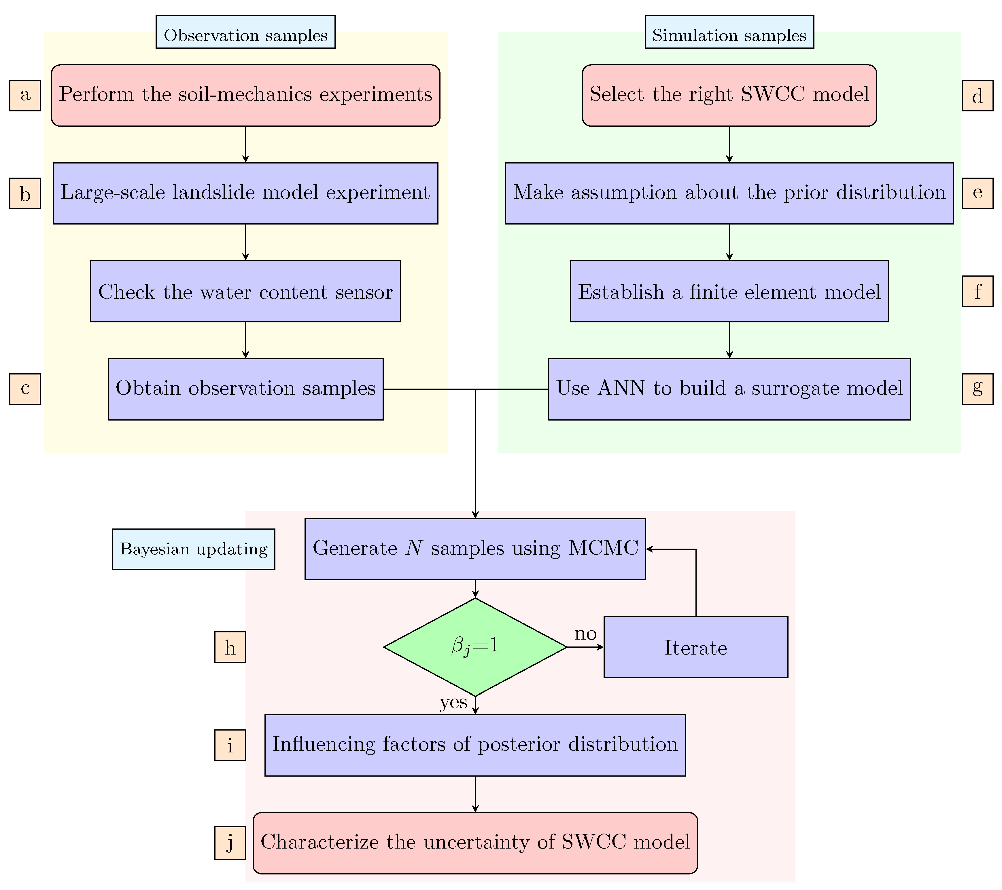
In this paper, the above-mentioned Bayesian updating method is used to calculate the SWCC model parameters. Bayesian updating is a method of statistical inference, in which as more evidence or information (in this paper is the observation samples) is obtained, Bayes’ theorem (Equation (2)) is used to update the probability of a hypothesis. First, the prior distribution of the SWCC model parameters is determined through reference research data or data from a SWCC experiment, as done in this work. Then, one uses the M–H method to generate a defined (large) number of random MCMC samples following a iterative calculation until β j = 1, and the posterior distribution is obtained. The M–H method is a powerful Markov chain method with which to simulate multivariate distributions. The main steps include initialization and iteration [34]. Figure 2 shows a flowchart for implementation of the proposed Bayesian approach schematically. The work done covers both the experimental results to feed the model (left branch on Figure 2), and the analysis methodology (right branch on Figure 2). The experimental data were obtained after basic soil mechanical experiments, to characterize the material of the landslide body, and a large-scale landslide model experiment, including water content sensors to measure in real-time the hydrodynamic process. The setup and results of the experiments are described in Section 4 and Section 5. Each step and its detailed description are summarized as follows.
  • Regarding the left branch, the main goal was to obtain Bayesian updating evidence (water content observation samples X o b s ) through the water content detection of large-scale landslide models:
    (a)
    Infiltration experiments and a triaxial experiment were carried out, and the material ratio of landslide body was determined to be 7:3 for soil:stone through these experiments.
    (b)
    Large-scale landslide models were built according to the layer-by-layer compaction method. The place where the sensor was buried was carefully compacted to avoid damage to the sensor.
    (c)
    After the landslide model and sensor were ready, the moisture content sensor was tested to determine the reliability of its data.
  • In the right branch, the main work was to obtain the Bayesian updating simulation samples ( X k ) through the finite element model:
    (d)
    The SWCC model was selected (VG model), and we analyzed the two model parameters within its range to observe their influences on the curve shape.
    (e)
    We assumed the prior distribution as normal or lognormal according to existing research. Then we determined the prior distribution of SWCC for the model parameters a and n, based on experimental data and research results.
    (f)
    A finite element (FE) numerical model was developed according to the large-scale landslide test; we evaluated the seepage flow under the conditions of the reservoir water level.
    (g)
    In the Bayesian updating process, it is necessary to call the FE model, taking a long time to obtain the large number of output values. Therefore, this paper used an artificial neural network (ANN) as a surrogate model to speed up the analysis.
  • In the lower part of the flowchart, the main work was to perform Bayesian updating by combining the water content observation samples ( X o b s ) of the large landslide model of the left branch and the simulation samples ( X k ) of the right branch:
    (h)
    The MCMC algorithm was used to generate N random samples that followed the posterior distribution of SWCC parameters and iteratively continued until β j = 1. We got the posterior distribution of SWCC model parameters (posterior most likely value, posterior mean, posterior standard deviation, etc.).
    (i)
    We analyzed the factors influencing the posterior distribution results, such as the number of observation datums, the prior distribution, and the observation data that changed over time.
    (j)
    We characterized the uncertainty of the SWCC model. For the parameters of the SWCC, the N samples generated from the MCMC algorithm were ranked, and a 95% confidence interval was obtained.
These steps were programmed, and MATLAB 2019b was used in this process. The programming of the program is divided into three steps: firstly, import the simulated and observed values; then use the MCMC algorithm to generate a large number of samples (100,000 sets of data in this program) to iterate for Bayesian updating; finally, the posterior distribution of the parameters of the SWCC model is visualized. In a different analysis case, the same analysis tools can be used so that geotechnical practitioners only need to provide laboratory or in-situ test results, prior knowledge (e.g., reasonable ranges of model parameters), and candidate SWCC models as inputs. The main advantage of the above method is that it can quickly check distributions of the posterior parameters of the SWCC.

4. The Large-Scale Landslide Model Experiment and Bayesian Updating

A large-scale landslide experiment was conducted using a soil–rock mixture and by monitoring the changes in water content to clarify the water migration during a landslide. The principle of numerical modeling, using an earlier developed model, is briefly explained. Simulations are presented and their results are compared to the experimental ones.

4.1. Experiment Setup

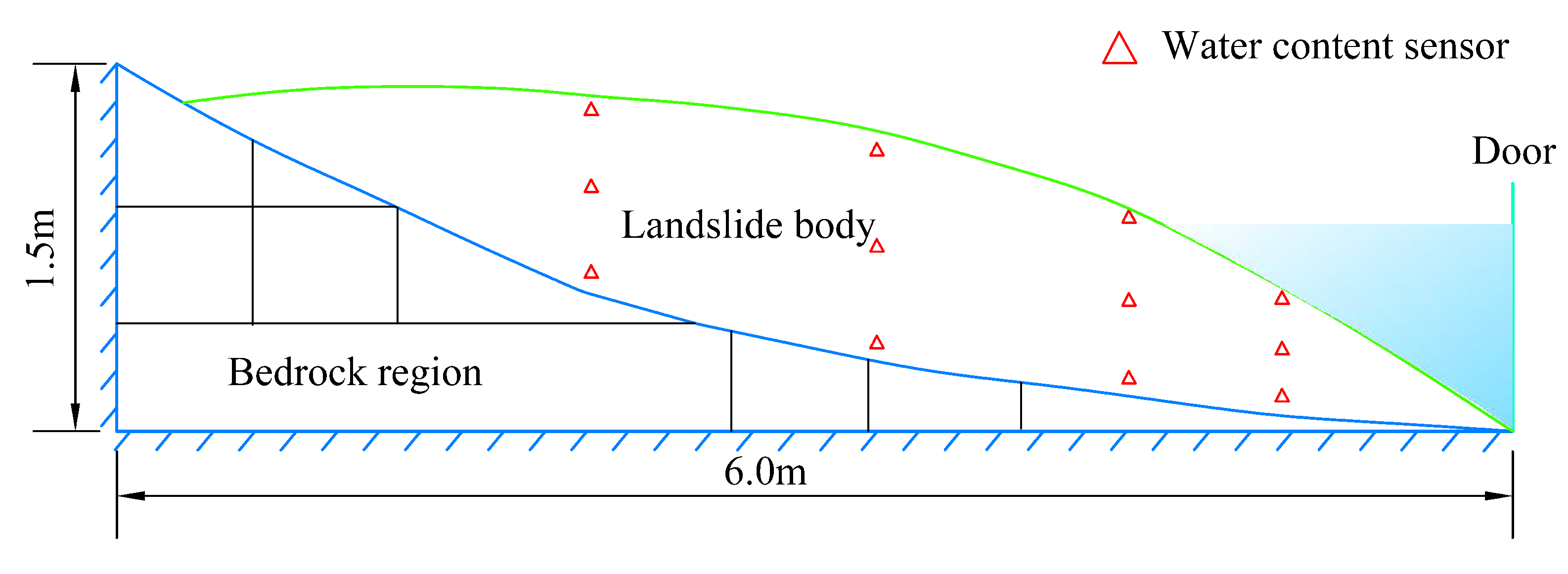
The experiments have been carried out in a large-scale landslide model experiment at The Key Laboratory of Geological Hazards and the Ministry of Education of the Three Gorges Reservoir Area of the Three Gorges University (China); the setup is shown in Figure 3. The model test platform was 6 m long, 0.8 m wide, and 1.5 m high. The door at the right end of the test platform could control the rise and fall of the reservoir water level. The landslide model was connected to external water supply pipes and drainage pipes. The speed at which the water level of the reservoir changed was adjusted by setting a flow valve.
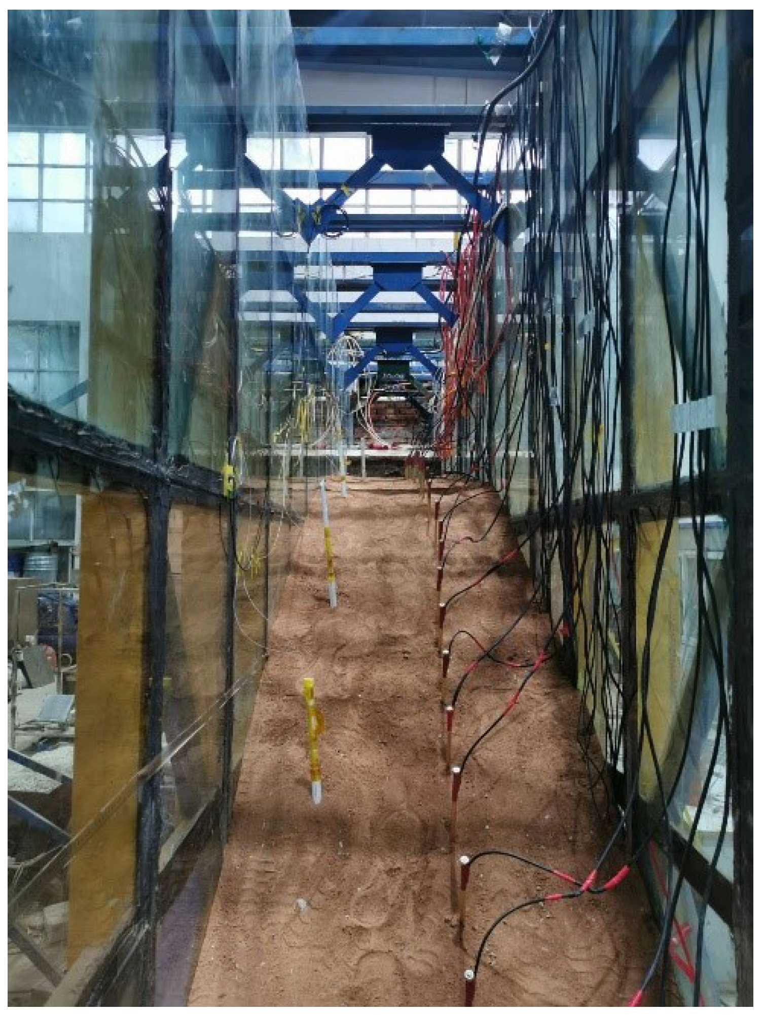
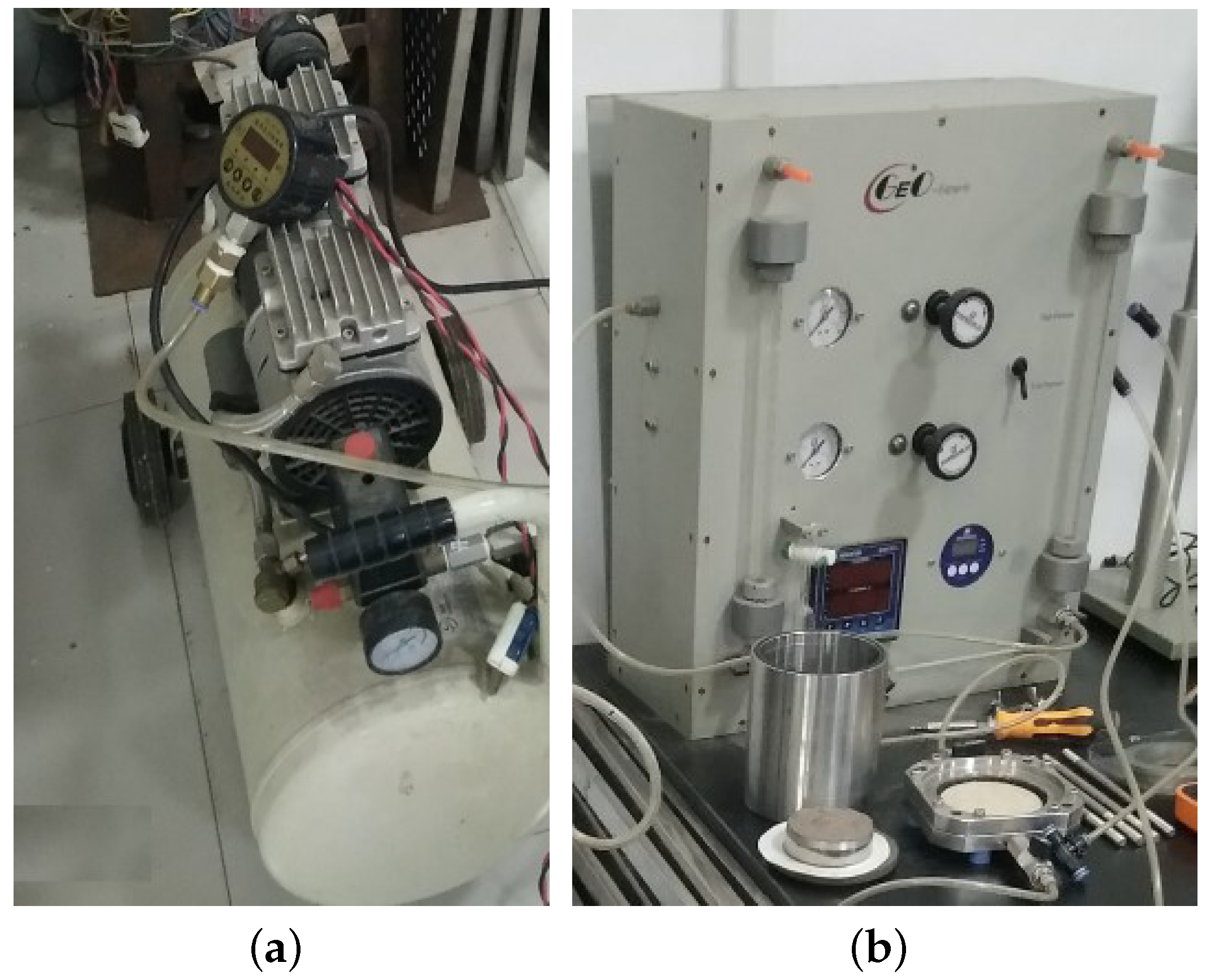
According to the nature of the landslide body in the Three Gorges reservoir area, the material of the landslide body was designed. The material used in the landslide body was composed of soil and small stones, and the ratio was 7:3. The landslide model test was completed according to the principle of landslide model forming. Considering the size of the model and the need to embed sensors, it was decided to choose the tamping method to build the landslide model. The sensors were embedded in the model in advance. The moisture content sensors were arranged in four sections, with 3 sensors in each section. Then we increased the water level of the reservoir to monitor the change of its water content. The overall landslide model is shown in Figure 4. In this figure, instruments for displacement monitoring and high-density electrical methods are included (the results are not used in this article.) In order to obtain the material parameters of the landslide model, a triaxial test and a constant head permeability coefficient experiment were carried out. A pressure plate instrument was used to obtain the characteristic curve of unsaturated soil water, as shown in Figure 5a,b. In this figure, the pressure pump and pressure plate instruments are displayed.
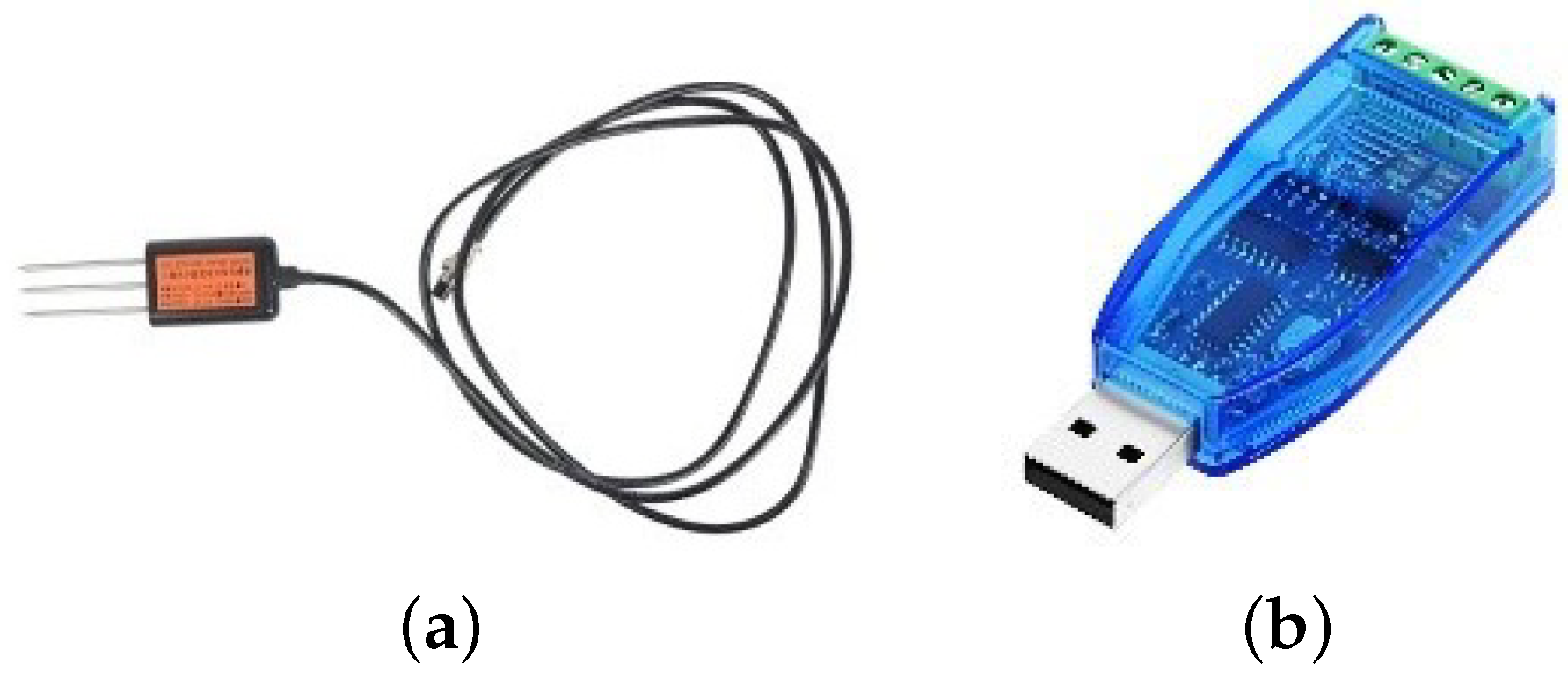
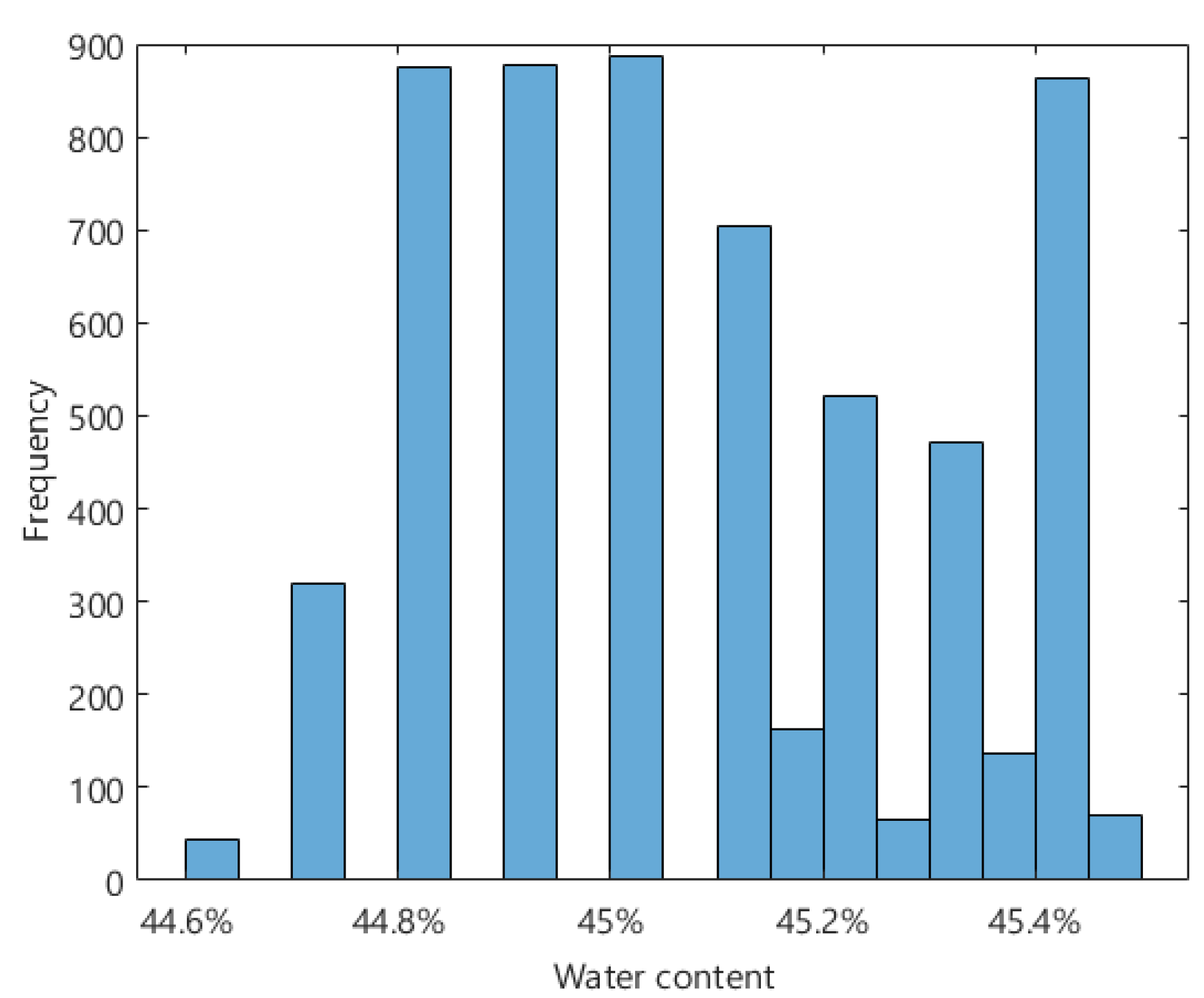
Sensors were used to obtain water content data in real time. Figure 6a shows the water content sensor. The power supply voltage of the sensor was 5 V, and the output signal type was RS485. The monitoring data of the water content sensor were saved when the water level was from 0.3 to 1 m. Figure 6b shows the sensor data interface. Its function was to convert RS485 signals into USB signals. Based on the Modbus protocol, the data acquisition software was developed using C# to save the water content data to the database. All sensors conducted data sampling and recording every 10 s. Figure 7 is a histogram representation of moisture sensor monitoring data. In this figure, the abscissa represents different moisture content, and the ordinate represents its frequency. These water content data were used as observation samples in Bayesian updating (specifically, as shown in Figure 2).

4.2. FEM Simulation

In the Bayesian updating process, a numerical model of the experimental setup is needed to provide simulation results. The SEEP/W software, a part of Geo Studio is a numerical simulation software for seepage analysis. In this study, Geo Studio software (2007) was used. It can mathematically simulate the real physical process of water flowing through the soil medium based on the finite element model. The equation used in the process is a steady-state seepage equation. The work of this section aims to model the seepage analysis of the landslide model in Figure 3 through the FEM. For this reason, a geometric model of a large-scale landslide model was built in FEM software. The purpose of this research was to study the seepage characteristics of landslides through FEM to simulate the changes in water content of landslides when the water level rises. We used SEEP/W software to develop and calibrate computer models of landslide model, and compare observed data with simulated data.
In the FE model process, the main steps are to establish a landslide model, set material parameters, divide calculation units, and set boundary conditions [35]. Firstly, SEEP/W was used for geometric modeling of the landslide model according to the dimensions in Figure 3. The material models and properties of the soil were put into saturated-unsaturated seepage model, defined with a seepage constitutive relationship requiring two functions: the permeability coefficient function and water content function (SWCC) [35]. In this process, the saturated permeability coefficient was set to 1 . 6 × 10 6 , and the SWCC parameters were set according to the prior distribution. Figure 8 shows the geometric model and the mesh used in this work. In this figure, the yellow area represents the landslide body. The unit accuracy of the finite element mesh was set to 0.1 m. The red part represents the boundary conditions. Two boundary conditions were set for the numerical model based on water level changes: water level boundary conditions and pressure boundary conditions. The boundary conditions of the model were a key component of the numerical analysis, and the ability to control the boundary conditions was also a direct reason for the powerful numerical analysis. In this process, the calculation method was the steady-state calculation, and the solver adopted the implicit solution method.
The FEM can evaluate water content values, depending on the input parameters (a,n) of the SWCC model. This results were the simulation samples used in Bayesian updating. The main purpose of this was to obtain the complete results of the FE model evaluation by SEEP/W software calculation, including water pressure, moisture content, etc. The results calculated by the SEEP/W software are analyzed and compared with the monitoring data of the landslide model in Section 4.1 to check for errors. The calculation of the SEEP/W software in this section also provides a model for the establishment of the surrogate model in the next section.

4.3. Surrogate Model

Bayesian updating requires two sets of data: one of experimental data, and the other of simulation data. The experimental data were obtained through the above-mentioned large-scale landslide model experiment, and the data are shown in Figure 7. The simulation data were calculated according to the FEM in Section 4.2. It took 690 h (about 29 days) to perform a complete Bayesian update calculation with the FEM, and 2 h to use the surrogate model (Intel(R) Core(TM) i5-5200U CPU @ 2.20 GHz, RAM 8.00 GB). Therefore, a surrogate model was used in this study to obtain the simulation value. The surrogate model is a commonly used optimization method in engineering problems. When the actual problem is very computationally intensive and difficult to solve, a simplified model with less computational complexity and a rapid solution can be used to replace the original model to speed up the optimization process. In this study, an ANN was used to build the surrogate model.
In order to improve the efficiency of Bayesian updating, we adopted the method of the surrogate model. We used an ANN to train the surrogate model. The ANN is an algorithm whose design is driven by the function of the human brain and its components. ANNs use nonlinear techniques, so they can be used to model highly complex and nonlinear systems. In this study, a fully connected feedforward multi-layer structure using a backpropagation momentum learning algorithm was adopted. This kind of ANN architecture usually consists of an input layer, some hidden layers, and an output layer. For us there were 10 neuron nodes used in each layer. Each node was interconnected to the nodes of the upper layer through adjustable weights, and horizontal, self-direction, or backward connection was not allowed. The calculation and expression ability of a single neuron is limited. However, when they are connected to each other, the entire network can model complex functions. The training pattern consists of a set of matched input and output vectors. The logical sigmoid function was used as the activation function. In order to develop the artificial neural network model, Neural Network Fitting toolbox and MATLAB R2019b were used. The Neural Network toolbox provides various parameters for neural network development, which can be selected flexibly. We set the distribution of the parameters of the SWCC model, and then used the SEEP/W software to calculate the value of the water content. We saved the SWCC model parameters and the generated water content data for the establishment of the surrogate model. The input data selected for this part were a array ( 2 × 1000 ) of SWCC parameters a and n, and the target array was water content data. In the training process, 70% of the data were used for training, 15% of the data for verification, and 15% of the data for testing. The training data were presented to the network during the training process, and the network was adjusted according to its errors. The verification data were used to measure the generalization of the network and stop training when the generalization stopped improving. The test data had no effect on training, so they provide an independent measurement of network performance during and after training. In this section, the number of hidden neurons was 10. Finally, we checked the error of the surrogate model built using an ANN.
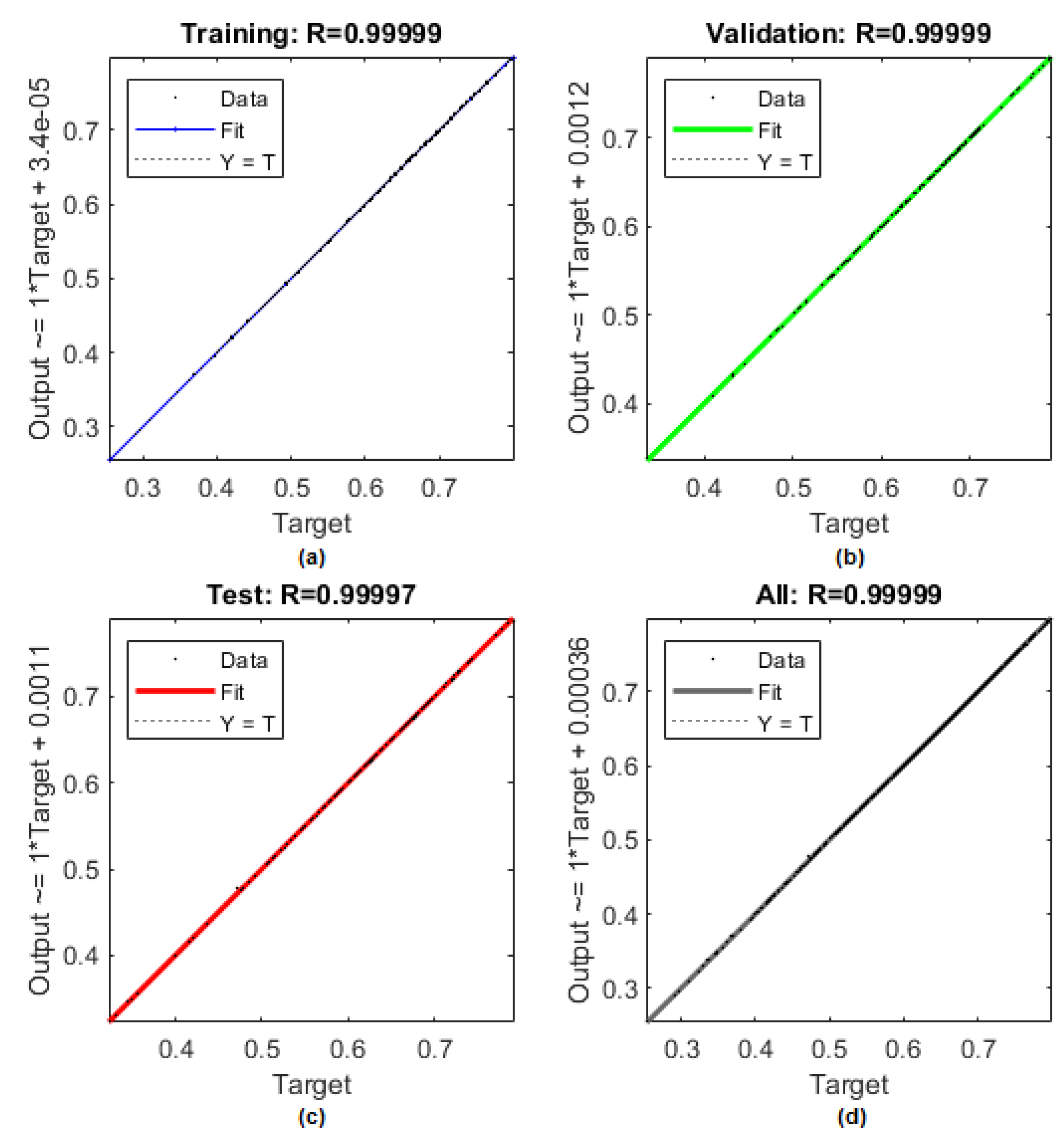
Figure 9 shows the regression diagram of the water content and SWCC parameters at specific points of the landslide model. In this figure, we can observe that all datasets were correctly fitted to the row. This shows that our neural network structure was correct, and it can also be used to predict the outputs of other input datasets. Figure 9a is the regression diagram of 70% of the training data. Figure 9b is the regression diagram of the 15% group of the validation data. Figure 9c is the regression diagram of the 15% group of test data. Figure 9d is the regression diagram of all data. The results of ANN prediction quality are detailed in Table 1. The goodness of fit (R) is close to 1 and the expected value of the mean square of the error (MSE) is small. The model results show that the ANN model can be used to predict the relationship between the water content at specific points of the landslide model and the parameters of the SWCC.

5. Results

5.1. Effect of Dataset Size on the Outcome of Bayesian Updating

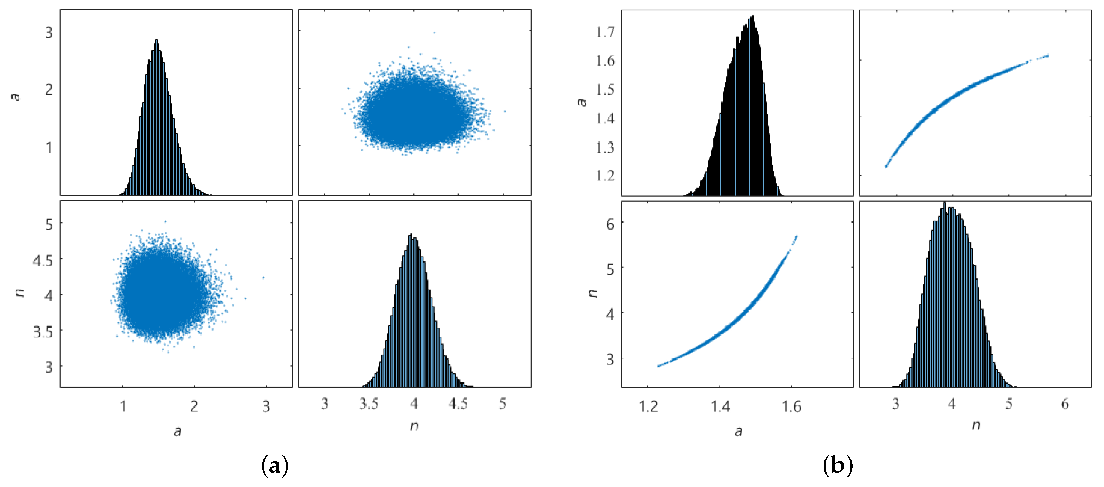
Using the surrogate model and the experimental data, the iterative Bayesian updating was done until the simulated value was close to the observed value. Bayesian updating is an iterative process. First, it sets the prior distribution of SWCC parameters and uses the MCMC algorithm to generate a large number of samples that obey the prior distribution. Then it performs iterative calculations, using surrogate models and experimental water cut monitoring data. Bayesian updating is performed until the simulated value is close to the observed value. For each iteration, a set of samples of SWCC parameters are generated. All the data of the iteration are presented into a plotmatrix, as shown in Figure 10a. In this figure, the top-left figure is the frequency diagram of parameter a, the bottom-right figure is the frequency diagram of parameter n, and the bottom-left and top-right figures represent the correlation. Figure 10b shows the distribution of SWCC parameters obtained by Bayesian updating, converged after 5 iterations (j = 5). This is the plotmatrix of the SWCC parameters after the fifth iteration.
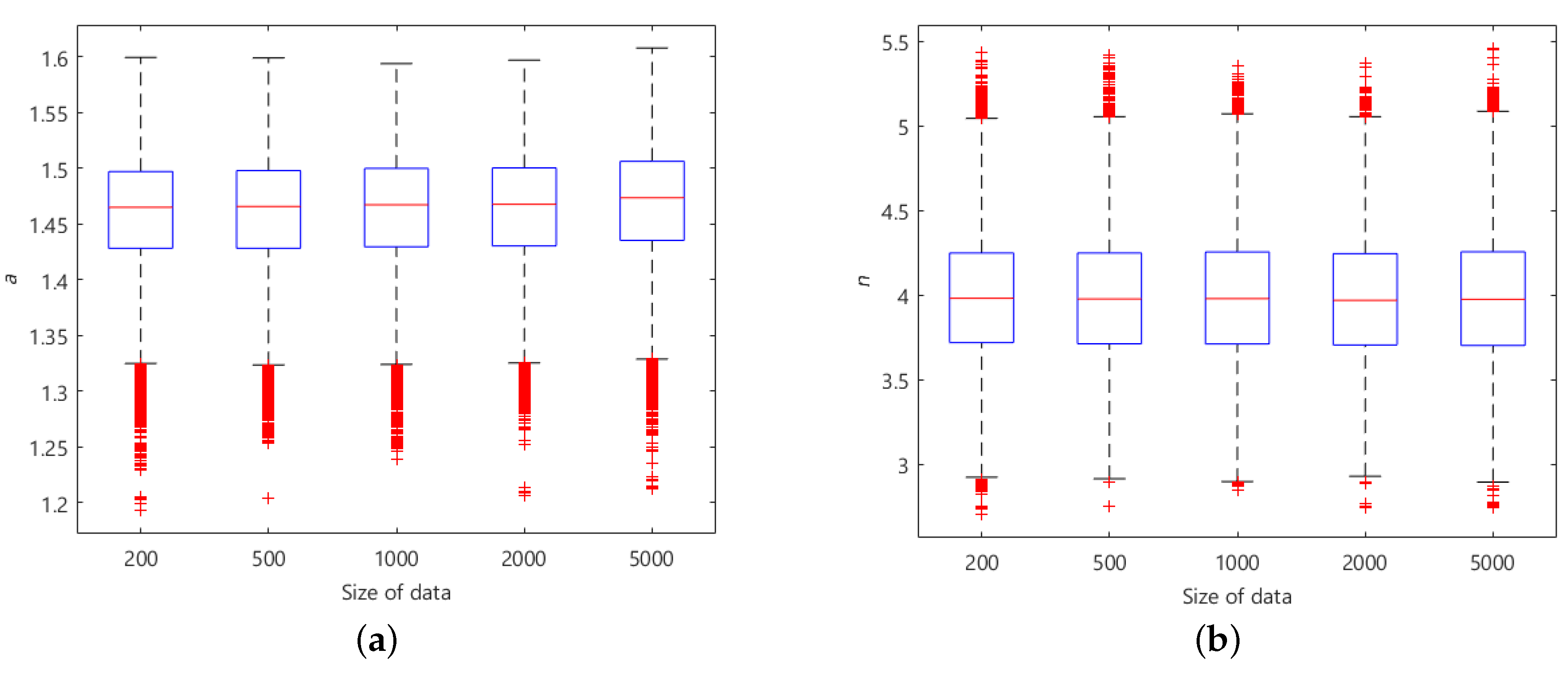
In order to study the changes in the posterior distribution when monitoring the increase in the amount of data, we used 200, 500, 1000, 2000, and 5000 sets of monitoring data to calculate the posterior distribution and analyze the results. As the amount of data increased, the trends of Bayesian updating results are shown in Figure 11, and the values of Bayesian updating results are shown in Table 2. In that figure, the red line represents the median, the upper and lower lines of the blue rectangle represent the upper and lower quartiles, the short red lines represent outliers, and the short black lines represent the minimum and maximum values. The trend of the change of parameter a is shown in Figure 11a. It can be seen that the median value of parameter a fluctuates around 1.46 and has a tendency to increase slightly. Outliers are distributed below the minimum value, indicating that the posterior distribution is left skewed. The trend of the change of parameter n is shown in Figure 11b. It can be seen that the median value of the parameter n fluctuated around 3.98. Outliers are distributed over the maximum value, indicating that the posterior distribution skewed right. When the number of data was 1000, the data of the posterior distribution were relatively stable. Therefore, in the following analysis, 1000 sets of observation data were used as samples to study the influence of the distribution type on the posterior distribution.

5.2. The Effect of Prior Distribution on the Outcome of Bayesian Updating

In this Bayesian updating process, the prior distribution of SWCC parameters a and n needs to be set first. In the previous analysis (Section 5.1) the prior distribution of variables a and n was adjusted to a lognormal distribution. The converged posterior distribution was analyzed and the most likely value, mean, and standard deviation of the parameter were evaluated. In Table 3, the results for the analysis with dataset size value 1000 are shown.
To investigate the effect that a different prior distribution has on the results, the prior distribution was changed to a normal distribution. The results are plotted in Figure 12, and the distribution parameters are shown in Table 3. Comparing the results of Table 3, the values of the parameters a and n are compatible within the deviations obtained.

5.3. The Effects of Six Stages on the Outcome of Bayesian Updating

During the experiment (see Section 4.1 for details), we set the data collection time interval of the moisture content sensor to 10 s. When the water level changed from 0.3 m to 1 m, six stages were selected to study the trend of the posterior distribution of SWCC parameters when the water level changed. With the monitoring data obtained over time, the trend of Bayesian updating results is shown in Figure 13, and the value of Bayesian updating results is shown in Table 4. In this boxplot, the red line represents the median, the upper and lower lines of the blue rectangle represent the upper and lower quartiles, the red short lines represent the outliers, and the black short lines represent the minimum and maximum values. The trend of the change of parameter a is shown in Figure 13a. It can be seen that the median value of parameter a fluctuates around 1.47 and has a tendency to increase slightly. Outliers are distributed above the maximum value. The trend of the change of parameter n is shown in Figure 13b. It can be seen that the median value of parameter n fluctuates around 3.98 and has a slightly lower trend.

5.4. Characterization of Uncertainty

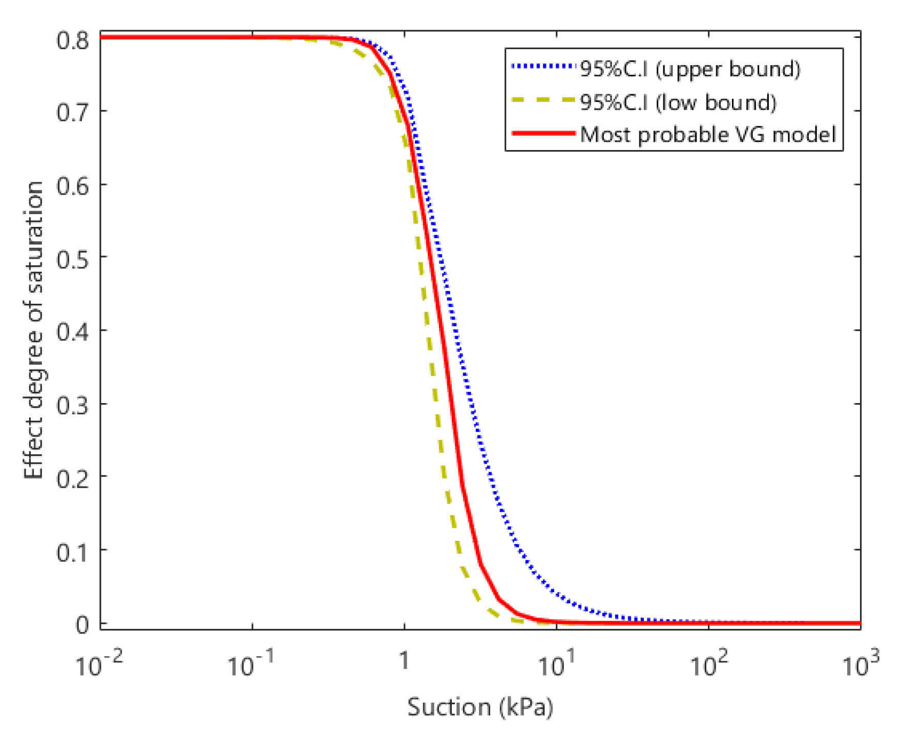
According to the previous results, it is possible to characterize the uncertainty of the model parameters. For a sufficiently large number of samples, and considering the minor effects caused by the selected prior distribution type and the time stage, the uncertainties obtained are reliable. Considering the VG model for the SWCC, the parameters a and n were evaluated with 100,000 MCMC samples and 95% confidence intervals (for 97.5% and 2.5% upper and lower bounds). The results are plotted on the curves in Figure 14. As can be seen in this figure, the most likely SWCC models were all within the 95% confidence interval. Therefore, the proposed method can reasonably determine the SWCC model based on limited experimental data and quantify the uncertainty of the SWCC model estimate.

6. Discussion

Although slight changes of SWCC parameters have minor effects on the stability of a landslide, they improve the accuracy of landslide reliability calculation. It is very necessary to conduct in-depth research on SWCC parameters. In previous studies, the main focus was on the SWCC model. We used indoor test data to select SWCC model [36]. Compared with the deterministic SWCC model, this paper took into account the uncertain factors caused by soil variability and unstable monitoring data. This paper mainly checked the parameters of SWCC based on the monitoring data of large-scale model tests.
This paper mainly describes the impacts of monitoring data volume, prior distribution type, and different stages on posterior distribution. Figure 11 and Table 2 show the effect of data volume from 200 to 5000 on the posterior distribution of SWCC model parameters. The left figure represents the prior distribution, and it can be clearly seen that the prior distribution is the same. The figure on the right represents the posterior distribution. As the number of observation samples increases, it has little effect on the posterior distribution of SWCC parameters. It can be seen from Table 2 that the results of the posterior distribution are very stable. Therefore, it is feasible to perform Bayesian updating of parameters using monitoring data. This makes it possible to realize the online SWCC parameter monitoring and analysis system. In the research, this study selected 1000 sets of data for Bayesian updating. Figure 10 and Figure 12 compare the effects of the prior distribution type on the results of the SWCC parameters’ posterior distributions. It can be clearly seen that the coefficient of variation is smaller when the prior distribution is lognormal. Therefore, when using monitoring data to perform Bayesian updating of SWCC parameters, it is more reasonable to set the prior distribution to the lognormal distribution to obtain the posterior distribution. Figure 13 and Table 4 show the changes in the posterior distributions of SWCC parameters with different stages. In this figure, it can be seen that the mean value of parameter a in the SWCC posterior distribution increases from 1.462 to 1.480, while the mean value of parameter n fluctuates from 3.985 to 3.983 (the fluctuation range is within 0.1). Due to the short monitoring time, the change to the posterior distribution is very subtle. In the follow-up research, the monitoring time could be extended to obtain the SWCC parameter change rule. Figure 14 shows the 95% confidence interval of the posterior distribution of SWCC. The most likely SWCC falls within the 95% confidence interval of its posterior distribution.
This paper studied the method of using landslide monitoring data to study SWCC parameters. However, due to the influences of many uncertain factors, the simulation model’s prediction and the real structural response often have certain errors. Therefore, it is necessary to verify the prediction accuracy of the simulation model in future research.

7. Conclusions

This paper presents a SWCC parameter calculation framework based on Bayesian landslide monitoring data theory. This method makes full use of prior information and limited monitoring data to determine the posterior information of SWCC model parameters. It characterizes the uncertainty of the SWCC model and is of great significance for reliability analysis. The influences of the dataset size, prior distribution type, and time-varying monitoring data on the result of posterior distribution were studied. Finally, the uncertainty of the SWCC model parameters was characterized. Taking the water content monitoring data of the large-scale landslide model test as an example, the effectiveness of this method is explained. The main conclusions from this study are as follows:
  • This paper proposes a Bayesian-based analysis method that can take the parameters’ uncertainty into account, and is different from conventional deterministic analysis methods. The feasibility of the Bayesian updating method in the monitoring data of a large landslide model was demonstrated. Through the Bayesian updating, the posterior value ranges of the SWCC parameters will be narrowed compared to the prior ones.
  • The Bayesian updating method has good application prospects in landslide monitoring. When the prior distribution is lognormal, the coefficient of variation of the posterior distribution is smaller than that of the normal distribution. The SWCC parameter a tends to increase when the posterior distribution changes with time.
  • In the process of Bayesian updating, a numerical simulation based in a FE model was used. Alternatively, a ANN surrogate model was also trained based on the FE model. This method can greatly improve the efficiency of Bayesian model updating—its accuracy being acceptable.

Author Contributions

Conceptualization, C.F. and M.B. (Michael Beer); data collection, C.F., X.L. and T.H.; methodology, C.F., M.B. (Matteo Broggi), and B.T.; software, C.F. and M.B. (Matteo Broggi); validation, C.F., B.X., and B.T.; data curation, C.F.; writing—original draft preparation, C.F.; writing—review and editing, S.B.; project administration, B.T.; funding acquisition, B.T. All authors have read and agreed to the published version of the manuscript.

Funding

This work is supported by the National Key Research and Development Program of China (2017YFC1501100), and the Research Fund for Excellent Dissertation of China Three Gorges University (2019SSPY005).

Acknowledgments

Thanks to the National Research Council and Three Gorges University for their support.

Conflicts of Interest

The authors declare no conflict of interest.

References

  1. Tan, X.; Wang, X.; Khoshnevisan, S.; Hou, X.; Zha, F. Seepage analysis of earth dams considering spatial variability of hydraulic parameters. Eng. Geol. 2017, 228, 260–269. [Google Scholar] [CrossRef]
  2. Zheng, D.; Huang, J.; Li, D.Q.; Kelly, R.; Sloan, S.W. Embankment prediction using testing data and monitored behaviour: A Bayesian updating approach. Comput. Geotech. 2018, 93, 150–162. [Google Scholar] [CrossRef]
  3. Wang, B.; Li, J.; Jiang, Q.; Yang, Y.; Feng, X.T. An improved FE-Meshfree method for solving steady seepage problems. Comput. Geotech. 2020, 119, 103223. [Google Scholar] [CrossRef]
  4. Guan, X.; Jha, R.; Liu, Y. Model selection, updating, and averaging for probabilistic fatigue damage prognosis. Struct. Saf. 2011, 33, 242–249. [Google Scholar] [CrossRef]
  5. Mia, M.; Dhar, N.R. Response surface and neural network based predictive models of cutting temperature in hard turning. J. Adv. Res. 2016, 7, 1035–1044. [Google Scholar] [CrossRef] [Green Version]
  6. Strauss, A.; Frangopol, D.M.; Kim, S. Use of monitoring extreme data for the performance prediction of structures: Bayesian updating. Eng. Struct. 2008, 30, 3654–3666. [Google Scholar] [CrossRef]
  7. Hsein Juang, C.; Luo, Z.; Atamturktur, S.; Huang, H. Bayesian updating of soil parameters for braced excavations using field observations. J. Geotech. Geoenviron. Eng. 2013, 139, 395–406. [Google Scholar] [CrossRef] [Green Version]
  8. Liu, W.; Luo, X.; Huang, F.; Fu, M. Uncertainty of the soil–water characteristic curve and its effects on slope seepage and stability analysis under conditions of rainfall using the Markov Chain Monte Carlo Method. Water 2017, 9, 758. [Google Scholar] [CrossRef] [Green Version]
  9. Lam, H.F.; Yang, J.; Au, S.K. Bayesian model updating of a coupled-slab system using field test data utilizing an enhanced Markov chain Monte Carlo simulation algorithm. Eng. Struct. 2015, 102, 144–155. [Google Scholar] [CrossRef]
  10. Rocchetta, R.; Broggi, M.; Huchet, Q.; Patelli, E. On-line Bayesian model updating for structural health monitoring. Mech. Syst. Signal Process. 2018, 103, 174–195. [Google Scholar] [CrossRef]
  11. Bi, S.; Broggi, M.; Beer, M. The role of the Bhattacharyya distance in stochastic model updating. Mech. Syst. Signal Process. 2019, 117, 437–452. [Google Scholar] [CrossRef]
  12. Van Genuchten, M.T. A closed-form equation for predicting the hydraulic conductivity of unsaturated soils. Soil Sci. Soc. Am. J. 1980, 44, 892–898. [Google Scholar] [CrossRef] [Green Version]
  13. Neuman, S.P.; Witherspoon, P.A. Finite element method of analyzing steady seepage with a free surface. Water Resour. Res. 1970, 6, 889–897. [Google Scholar] [CrossRef] [Green Version]
  14. Leong, E.C.; Rahardjo, H. Review of soil-water characteristic curve equations. J. Geotech. Geoenviron. Eng. 1997, 123, 1106–1117. [Google Scholar] [CrossRef] [Green Version]
  15. Thu, T.M.; Rahardjo, H.; Leong, E.C. Elastoplastic model for unsaturated soil with incorporation of the soil-water characteristic curve. Can. Geotech. J. 2007, 44, 67–77. [Google Scholar] [CrossRef]
  16. Fredlund, D.G.; Xing, A. Equations for the soil-water characteristic curve. Can. Geotech. J. 1994, 31, 521–532. [Google Scholar] [CrossRef]
  17. Gardner, W. Some steady-state solutions of the unsaturated moisture flow equation with application to evaporation from a water table. Soil Sci. 1958, 85, 228–232. [Google Scholar] [CrossRef]
  18. Li, D.Q.; Qi, X.H.; Phoon, K.K.; Zhang, L.M.; Zhou, C.B. Effect of spatially variable shear strength parameters with linearly increasing mean trend on reliability of infinite slopes. Struct. Saf. 2014, 49, 45–55. [Google Scholar] [CrossRef]
  19. Li, D.Q.; Wang, L.; Cao, Z.J.; Qi, X.H. Reliability analysis of unsaturated slope stability considering SWCC model selection and parameter uncertainties. Eng. Geol. 2019, 260, 105207. [Google Scholar] [CrossRef]
  20. Johari, A.; Talebi, A. Stochastic Analysis of Rainfall-Induced Slope Instability and Steady-State Seepage Flow Using Random Finite-Element Method. Int. J. Geomech. 2019, 19, 04019085. [Google Scholar] [CrossRef]
  21. Han, Z.; Vanapalli, S.K. Model for predicting resilient modulus of unsaturated subgrade soil using soil-water characteristic curve. Can. Geotech. J. 2015, 52, 1605–1619. [Google Scholar] [CrossRef]
  22. Brutsaert, W. Probability laws for pore-size distributions. Soil Sci. 1966, 101, 85–92. [Google Scholar] [CrossRef]
  23. Chiu, C.; Yan, W.; Yuen, K.V. Reliability analysis of soil–water characteristics curve and its application to slope stability analysis. Eng. Geol. 2012, 135, 83–91. [Google Scholar] [CrossRef]
  24. Ching, J.; Chen, Y.C. Transitional Markov chain Monte Carlo method for Bayesian model updating, model class selection, and model averaging. J. Eng. Mech. 2007, 133, 816–832. [Google Scholar] [CrossRef]
  25. Patelli, E.; Govers, Y.; Broggi, M.; Gomes, H.M.; Link, M.; Mottershead, J.E. Sensitivity or Bayesian model updating: A comparison of techniques using the DLR AIRMOD test data. Arch. Appl. Mech. 2017, 87, 905–925. [Google Scholar] [CrossRef] [Green Version]
  26. Wang, L.; Cao, Z.J.; Li, D.Q.; Phoon, K.K.; Au, S.K. Determination of site-specific soil-water characteristic curve from a limited number of test data—A Bayesian perspective. Geosci. Front. 2018, 9, 1665–1677. [Google Scholar] [CrossRef]
  27. Kelly, R.; Huang, J. Bayesian updating for one-dimensional consolidation measurements. Can. Geotech. J. 2015, 52, 1318–1330. [Google Scholar] [CrossRef] [Green Version]
  28. Papaioannou, I.; Straub, D. Reliability updating in geotechnical engineering including spatial variability of soil. Comput. Geotech. 2012, 42, 44–51. [Google Scholar] [CrossRef] [Green Version]
  29. He, L.; Liu, Y.; Bi, S.; Wang, L.; Broggi, M.; Beer, M. Estimation of failure probability in braced excavation using Bayesian networks with integrated model updating. Undergr. Space 2019. [Google Scholar] [CrossRef]
  30. Tian, M.; Li, D.Q.; Cao, Z.J.; Phoon, K.K.; Wang, Y. Bayesian identification of random field model using indirect test data. Eng. Geol. 2016, 210, 197–211. [Google Scholar] [CrossRef]
  31. Phoon, K.K.; Tang, C. Characterisation of geotechnical model uncertainty. Georisk Assess. Manag. Risk Eng. Syst. Geohazards 2019, 13, 101–130. [Google Scholar] [CrossRef]
  32. Beck, J.L.; Katafygiotis, L.S. Updating models and their uncertainties. I: Bayesian statistical framework. J. Eng. Mech. 1998, 124, 455–461. [Google Scholar] [CrossRef]
  33. Katafygiotis, L.S.; Beck, J.L. Updating models and their uncertainties. II: Model identifiability. J. Eng. Mech. 1998, 124, 463–467. [Google Scholar] [CrossRef]
  34. Chib, S.; Greenberg, E. Understanding the metropolis-hastings algorithm. Am. Stat. 1995, 49, 327–335. [Google Scholar]
  35. Arshad, I.; Baber, M. Finite element analysis of seepage through an earthen dam by using geo-slope (SEEP/W) software. Int. J. Res 2014, 1, 612–619. [Google Scholar]
  36. Wang, L.; Tang, L.; Wang, Z.; Liu, H.; Zhang, W. Probabilistic characterization of the soil-water retention curve and hydraulic conductivity and its application to slope reliability analysis. Comput. Geotech. 2020, 121, 103460. [Google Scholar] [CrossRef]
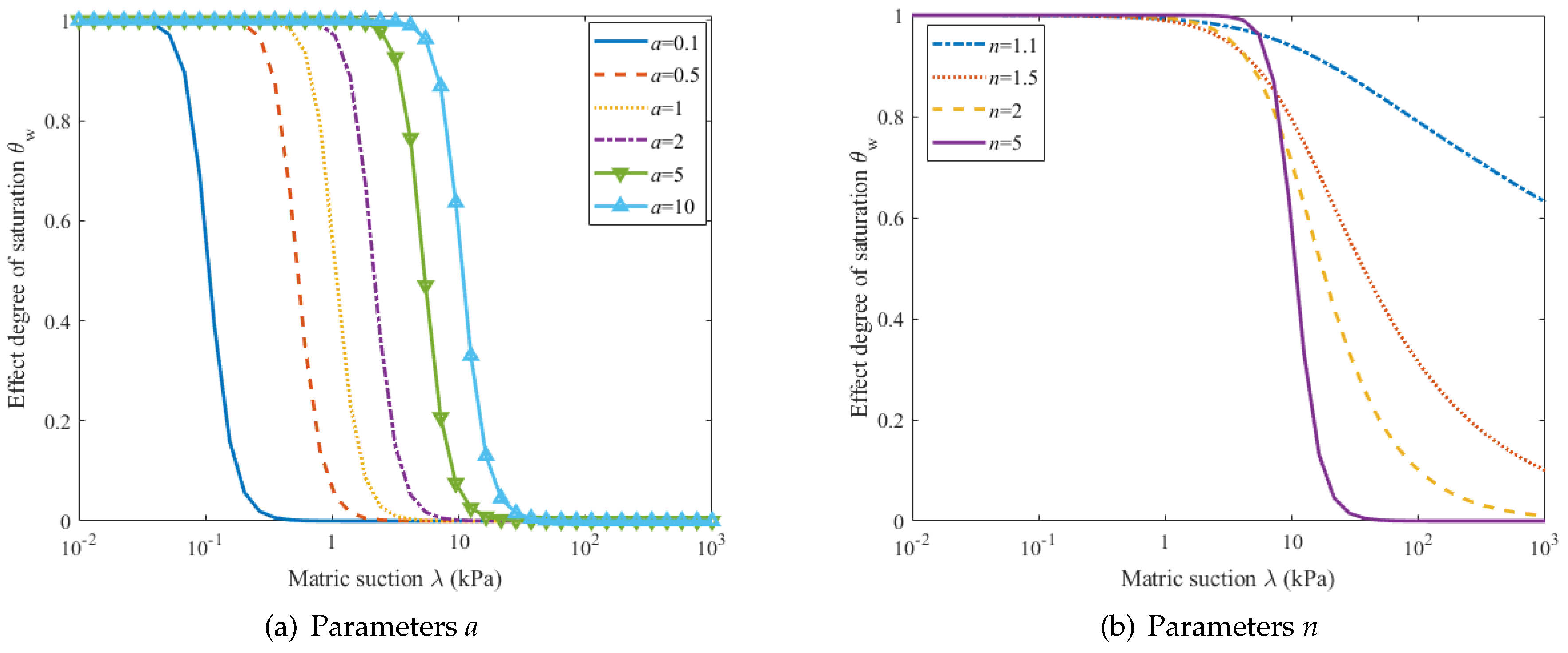
Figure 1. (a) The influence of parameters a on the soil–water characteristic curve (SWCC), and the n is 5 in this figure; (b) The influences of parameters n on the SWCC equation, and the a is 2 in this figure.
Applsci 10 05526 g001
Figure 2. Flowchart of the Bayesian updating procedure.
Applsci 10 05526 g002
Figure 3. The side view of the landslide model and configuration of instruments in the experiment. A drawing of the configuration of the experimental model, showing the bedrock region (within blue lines), the landslide body region (below the green line), and the embedded sensors to monitor the water content.
Applsci 10 05526 g003
Figure 4. A picture of the landslide model built indoors, from a frontal view: the model was 1.5 m (height) ∗ 0.8 m (width). The water content sensor is inside the landslide body (not visible; the actual water content sensor is shown in Figure 6a).
Applsci 10 05526 g004
Figure 5. Pressure plate instrument: (a) pump; (b) pressure gauge.
Applsci 10 05526 g005
Figure 6. (a) Water content sensor (the rated voltage was 5 V); (b) signal conversion device (converting the RS485 signal to USB signal).
Applsci 10 05526 g006
Figure 7. Monitoring data of water content.
Applsci 10 05526 g007
Figure 8. Mesh generation of finite element model (FEM).
Applsci 10 05526 g008
Figure 9. Neural network training regression: (a) The regression diagram of the 70% group of the training data; (b) The regression diagram of the 15% group of the validation data; (c) The regression diagram of the 15% group of test data; (d) The regression diagram of all data.
Applsci 10 05526 g009
Figure 10. Results of using 1000 sets of water content monitoring data to update: (a) prior distribution; (b) posterior distribution.
Applsci 10 05526 g010
Figure 11. Impact of data volume on update results: (a) Parameter a; (b) parameter n.
Applsci 10 05526 g011
Figure 12. Update results when the prior distribution is a normal distribution: (a) prior distribution; (b) posterior distribution.
Applsci 10 05526 g012
Figure 13. The influence of the monitoring value at different time stages on the update result: (a) parameter a; (b) parameter n.
Applsci 10 05526 g013
Figure 14. The 95% confidence interval of VG obtained from the Bayesian updating.
Applsci 10 05526 g014
Table 1. The results of the prediction with the artificial neural networks (ANN).
SamplesMSER
Training7001.43430 × 10 7 9.99991 × 10 1
Validations1501.67754 × 10 7 9.99989 × 10 1
Testing1505.56267 × 10 7 9.99968 × 10 1
Table 2. Impact of dataset size on update results.
Most Probable VG Model ParametersPosterior MeanPosterior Standard Deviation
Dataset Size a n a n a n
2001.473.941.4593.9810.0480.363
5001.483.921.4603.9800.0480.359
10001.493.851.4623.9850.0480.364
20001.493.851.4643.9880.0480.367
50001.503.841.4683.9780.0480.364
Table 3. Impact of prior distribution on update results.
Most Probable VG Model ParametersPosterior MeanPosterior Standard Deviation
Type a n a n a n
normal distribution1.484.061.4623.9870.0480.367
lognormal distribution1.493.851.4623.9850.0480.364
Table 4. Impacts of different stages on update results.
Most Probable VG Model ParametersPosterior MeanPosterior Standard Deviation
Stage a n a n a n
11.493.851.4623.9850.0480.364
21.4834.031.4653.9780.0480.362
31.4864.011.4693.9840.0470.360
41.4983.981.4723.9830.0480.369
51.5083.801.4763.9850.0470.364
61.5133.821.4803.9830.0470.365