Nonlinear Dynamics of Swinging Clapper Bells under Arbitrary or Resonant Forcing Functions

Featured Application

Innovative algorithms to solve the system of nonlinear ordinary differential equations governing free and forced oscillations of swinging clapper bells, duly considering the clapper impacts, are discussed. These algorithms provide the time histories of the relevant motion parameters of bell and clapper: rotations, angular velocities, angular accelerations, radial excitations at the pivots, and so on, also considering friction and viscous damping, if present. For its generality, the proposed method is particularly suitable not only to assess the bell “ringability”, but also the determine the excitation transmitted by the swinging bell to the supporting structures under arbitrary forcing functions.

Abstract

Study of swinging clapper bells involves aspects encompassing sound and acoustic engineering, mechanical engineering, and structural engineering. From the musical point of view, clapper bells are directly played idiophone instruments, where the playing device, the clapper, although directly excited, is not explicitly controlled by the bell ringer. The achievement of a clear and optimal sound mainly depends on the acoustic characteristics of the bell and on the regularity of the clapper strokes, which is not only governed by the ringing style and the relevant parameters of clapper and bell but also by the real time corrections to the excitation introduced by trained bell ringers. In fact, despite centuries of experience allowed to optimize the bell performances, standardizing proportions and mounting arrangements, effective sound control requires some fine tuning of the forcing function. Another crucial topic, especially in view of assessing existing structures, regards the evaluation of time histories of the actions transmitted by the bell to the pivots and the study of the interactions between the bell and the supporting structures, belfries, and bell-towers. “Ringability” of swinging bells and bell-structure interactions are usually tackled in the framework of rigid body dynamics, so arriving at an initial value problem, governed by a system of two second order nonlinear ordinary differential equations (ODEs), whose solutions are piecewise-defined functions. In the relevant literature, numerical solutions of the system are commonly sought using built-in algorithms provided in advanced software packages; since the use of such general algorithms is subject to some restrictions, especially regarding the forcing functions, validity of the results is often limited. The present study focuses on an innovative procedure to solve the equations of motion. The method, extremely fast and effective, is based on original numerical explicit-implicit predictor-corrector integration algorithms with constant time step, duly validated reproducing the outcomes of relevant reference case studies. Each time the clapper strikes the bell a new “piece” of the solution is initialized, so avoiding user interventions in the elaboration phase. Independently on the oscillation amplitude and on the duration of the considered time interval, the algorithms can successfully manage undamped oscillations; friction and viscosity damped oscillations; free oscillations in transient and stationary phases; and can be applied also to solve stiff equations. Furthermore, the capability of the proposed methods to deal with arbitrary forcing functions is particularly innovative. The outcomes of relevant case studies, regarding the oscillations of the old tenor bell of the Great St. Mary church in Cambridge, confirm the potentialities of the method, also highlighting some topical issues, involving, for example, the assessment of damping equivalence. Finally, a pioneering feature of the algorithms is their ability to handle and to define “resonant” forcing functions, continuously tuning the frequency of the excitation to the natural frequency of the oscillation, according to the oscillation amplitude.

1. Introduction

Since their origin, dating in China back to around the 3rd millennium BC [1], bells have been widely used as musical percussion instruments for religious rites and other relevant events.

Starting from the early Middle Ages, bells knew a large diffusion also in Europe and in the Christian world, so that tower bells became a normal addition of churches and other important municipal or civil buildings.

From the musical point of view, according to the Musical Instrument Museums Online (MIMO) revision [2,3] of the Hornbostel–Sachs classification [4] the bells are directly struck idiophone instruments, that vibrate “without requiring stretched membranes or strings”. The sophisticated categorization of bells given in [2] is a function of the mounting, of the position and of the way they are struck, but for the aim of the study a more rudimentary distinction is enough.

Depending on the position, bells can be classified as:

• resting bells, whose “cup is placed on the palm of the hand or on a cushion; its mouth faces upwards”, not relevant for the aim of the study, or
• suspended bells.

Suspended bells are grouped in three main subcategories, depending on the way they are struck:

b1.

bells, often without internal clapper, struck from outside with a separate hammer,

b2.

clapper bells, characterized by an internal clapper,

b3.

bells with attached external clapper.

Oriental religions generally utilize bells belonging to type b1 or b3; on the contrary, in the Christian context, church bells generally fall in type b2, even if, in particular cases, or events, they can also be struck from outside.

Depending on the excitation, clapper bells can be rung in two different ways. In fact, the vibrations can be excited by clapper strokes indirectly caused by the swinging bell, or by chimes, i.e., leaving the bell quite motionless and directly striking the clapper against it. The latter technique is typical of the Orthodox Church tradition, while in the rest of Christianity swinging bells are the rule, even if in most cases, for conservation purposes, they are chimed via motorized devices.

Swinging clapper bells raise intricate mathematical and physical problems, covering sound and acoustic engineering, mechanical engineering, and structural engineering as well.

As already noted, the swinging bell is a peculiar musical instrument played with a device, the clapper, whose movements, although directly excited, are not explicitly controlled by the bell ringer. The achievement of a clear and optimal sound thus relies not only on the acoustic characteristics of the bell but also on the regularity of the clapper strokes, which depends on the parameters of clapper and bell governing the equations of motion. Such parameters have been empirically tuned over centuries of practical experience leading to standardized proportions, nevertheless, in some cases, the sound control could result extremely difficult even when the bells are driven by well experienced bell ringers. In fact, if on the one hand, in case the bells are manually rung, some odd behavior can be compensated by skilled bell ringers duly modifying the excitation, on the other, in case the bells are swung by motors, fine real time adjustments are practically precluded.

It must also be underlined that different layouts are adopted to suspend the bells, mainly depending on: the ringing technique; the weight of the joke, eventually contributing to counterweight the bell; the position of the bell pivot with respect to the center of gravity of the bell; the distance between the clapper pivot and the bell pivot. The discussion of the rationale and consequences of different arrangements is out of the scope of the present paper, but it must be stressed that distinctive features of bells are also influenced by the technique intended for ringing them.

As described in [5], generally, they can be distinguished:

• the “flying clapper” ringing technique, mainly used in continental Europe, except the Iberic peninsula and north Italy,
• the full circle techniques, like the English full circle ringing or change ringing technique [6,7,8,9], and the Italian “Bolognese”, “Veronese”, and “Ambrosiano” styles,
• the Spanish system, typically used in Iberic peninsula.

In the “flying clapper” technique, the maximum oscillation of the bell, which is not counterweight, is around 90°, although in some cases it can attain 135°, and the clapper strikes the bell on the upper part of the mouth. Occasionally, in France, Belgium, and the Netherlands also the opposite “falling clapper” scheme is adopted, where the clapper strikes the lower part of the mouth.

The full circle techniques are based on alternate full circle oscillations, which facilitate the sound control. The bells are firstly driven in the upward position, where they are briefly stopped with the help of suitable devices or even manually, and then put in oscillations, which are maintained accurately adjusting the excitation. The English full circle and the Bolognese style use unbalanced bells, on the contrary “Veronese” and “Ambrosiano” styles adopt balanced bells.

In the Spanish system, balanced bells continuously rotate full circle in one direction [10,11,12,13].

From the above considerations, it clearly emerges that study of swinging bells can involve:

• the assessment of the acoustic characteristics of the bell itself, intended as a musical instrument,
• the quality and the precision of the sound, depending on the ease of controlling the clapper impacts during the oscillations, and
• the interactions between the swinging bell and the supporting structures: belfry and bell tower.

The acoustics of the bells is a very specialized topic, outside the scope of the present study, therefore it will not be further discussed. The interested reader can find some basic information about theoretical, experimental, or numerical acoustic studies in [14,15,16,17].

Truly, the ease of controlling the impacts significantly influences the acoustic performance of the bell; in fact, as remarked in [18], “the “ringability” of bells depends not only on the linear acoustics of the modes and natural frequencies of the bells but also on the rotational dynamics of the bell and clapper, interacting through impact each time the clapper strikes the bell surface.”

The inertia forces due to the swinging of the bell play a crucial role in dynamic identification [19] or assessment of existing bell towers [8,9,10,11,12,13,20,21,22,23,24,25], especially when the frequency of the bell oscillations is in the neighborhood of the relevant natural frequencies of the tower. Some analytical solutions for bell-tower interaction are given in [13], considering free oscillations and different mounting systems. However, some studies focus on the seismic response of the bell itself [26].

The time histories of bell and clapper rotations and support reactions are commonly studied in the framework of the Lagrangian mechanics, following the approach proposed by Lagrange [27,28], which is described in detail in every modern book of theoretical mechanics [29,30,31]. The analytical model of the bell, based on rigid body dynamics, originally suggested by Veltmann [32] in the 19th century, was recovered in the late 20th century by Threlfall and Heyman [33], who also suggested a simple experimental method to derive the inertia forces transmitted by full circle ringing bells. Since then, several studies have been carried out, shortly discussed in the following.

A recurrent simplification disregards the presence of the clapper; the bell motion is thus governed by the ordinary differential equation (ODE) of the physical pendulum, depending on two independent initial conditions. But, as better illustrated in Section 2, more refined approaches lead to a system of two second-order nonlinear ODEs. The solutions of that system are the time histories of bell and clapper rotations, provided that four independent initial conditions are given.

It must be underlined that, except in the case of small amplitude oscillations, when the physical pendulum equation can be linearized, the ODEs are always nonlinear, even if springs and dampers are not present. That peculiarity significantly distinguishes the swinging bell model from the simple harmonic oscillator, whose behavior is nonlinear only if nonlinear terms are explicitly introduced, like, for example, nonlinear restoring forces or springs in the Duffing oscillator [34]. Sometimes Duffing oscillator has been also used to approximate the nonlinear pendulum equation, based on the McLaurin expansion of the sinus function, but these aspects are outside the scope of the study.

To solve the swinging clapper bell problem, many different approaches have been proposed, alternatively concentrating the attention on the bell-clapper interactions or on the bell-tower excitation. Frequently, aiming to obtain convenient expressions of the equations, drastic simplifications are introduced, so arriving at suitable analytical or numerical solutions.

Noteworthy simplifications, often combined, may include:

• neglecting the clapper, so that the bell reduces to the already cited physical pendulum,
• neglecting the damping, thus considering only undamped oscillations,
• considering only viscous damping,
• disregarding external forces, thus considering only free oscillations,
• disregarding the transient phase, dealing with forced oscillations,
• suitably modifying the forcing functions to obtain “workable” equations from the analytical [22], or the numerical point of view [35,36,37,38],
• adopting simplified models to describe the impact of the clapper on the bell.

However, if analytical solutions are available only for special cases, also usual numerical approaches can result unsatisfactory. In fact, numerical solutions reported in the relevant literature are commonly obtained adopting built-in algorithms for the solutions of ODEs, available in advanced software packages, like Matlab^®. These algorithms are frequently based on Runge–Kutta methods. The availability of such sound and validated algorithms, characterized by clearly defined limitations, is certainly beneficial, but resorting to them involves rather evident disadvantages, because these general methods are scarcely flexible and not easily adaptable to handle specific problems.

Moreover, hypothesizing viscous damping only and assuming special forcing functions, the field of application of these “traditional” approaches sensibly reduces.

With regards to the previous remarks, it must be stressed, on one hand, that other kinds of damping, like friction damping, can play a key role and on the other, that different forcing functions can be envisaged in stationary or transient phases, also depending on the type of excitation−manual or automatic, and on the type of the motorization: linear, or rotating, or even contactless, if any.

Since the pivots are generally equipped with bushes or roller bearings, in which dissipative forces depend on the radial reaction forces, friction damping appears as the most appropriate model. Nevertheless, it is common practice to adopt an “equivalent” viscous damping model, so drastically simplifying the equations. Unfortunately, as confirmed by the outcomes of the study, the equivalence holds on a limited range of oscillation amplitudes, so that the parameters of the equivalent model should be continuously adjusted and adapted, depending on the actual situation.

Regarding the forcing functions, it is noteworthy that a typical transient is the starting phase, in which the bell is set in motion and suitably excited until a pre-established configuration is achieved. Especially in the case that the bells are manually driven or contactless excitations are adopted, the forcing functions are often optimized to be “resonant”, i.e., continuously and suitably tuned by an external device or by a trained bell ringer to match the instantaneous natural frequency of the system, which is a function of the amplitude of the oscillation.

For these reasons, an ideal and fully featured method to solve the ODEs of motion should allow:

• to take into account both viscous and friction damping,
• to consider “arbitrary” forcing function,
• to determine the solution in both stationary and transient phases,
• to introduce or to deduce “resonant” excitations, automatically tuned on the instantaneous natural frequency of the system.

In addition, the method should work also with “stiff equations”.

The aim of the study is the setup of an original all-purposes general procedure to solve the system of ODEs describing the motion of the bell and of the clapper.

The proposed algorithms discussed in Section 6 are based on explicit-implicit predictor-corrector integration methods with constant time step, directly operating on the ODEs system. They do not require any preliminary manipulation of the equations themselves, with evident advantages. To highlight their flexibility, two slightly different versions of the algorithms are presented:

• a moderately simplified version, in which the prediction-correction phase works only on the rotations of bell and clapper,
• the complete, more refined, version, in which the convergence is improved thanks to an additional prediction-correction phase regarding the angular velocities and the angular accelerations too.

The paper is organized as follows:

• Section 2 illustrates the deduction of the ODEs governing the problem.
• Section 3 refers to the model of the clapper to bell impact and how it is considered in the equations.
• Section 4 illustrates the friction and viscous damping models, while
• Section 5, considering the dissipative moments corresponding to damping phenomena, describes the general form of the nonlinear system of ODEs.
• Section 6 illustrates in detail the implementation of the proposed algorithms.
• Section 7 deals with the validation of the proposed method, checking its capability to reproduce some relevant theoretical or experimental results. To enrich the comparison, the convergence of the proposed algorithms is assessed, and its dependence on the time step and other influencing parameters is critically discussed, also considering “stiff” equations. Of course, that section is not essential for the understanding of the remaining parts of the paper.
• Section 8 considers a significant case study, consisting in the old tenor bell of the Great St. Mary’s church in Cambridge, whose characteristics are precisely reported in [17]. Several relevant situations are analyzed, considering damped or undamped conditions; free oscillations; forced oscillations; stationary or transient phases; different initial conditions; demonstrating the main features and the potentialities of the proposed algorithms.
• Section 9 summarizes the main conclusions, envisaging further developments.

The novel approach and the algorithms proposed in the paper allow one to overcome the limitations affecting the “traditional” approaches proposed until now; in fact, besides satisfying all the previously recalled requisites (a−c), they are also able to derive or to define resonant excitations and to solve stiff equations, as well. Independently on the oscillation amplitude and on the duration of the considered time interval, the algorithms can successfully manage undamped oscillations; friction and viscosity damped oscillations; free oscillations in transient and stationary phases; and can be applied also to solve stiff equations. Furthermore, the capability of the proposed methods to deal with arbitrary forcing functions is particularly innovative.

Typical outcomes of the method are time histories and phase plots in transient and stationary phases of relevant parameters under “arbitrary” forcing functions, including the excitations transmitted to the belfry and the bell tower through the supports. Even in the paper the attention is mainly concentrated on “unbalanced” swinging systems; the proposed methods apply also to the other system previously cited.

2. The Governing Equations

In the classical Lagrange–Euler approach, the equations of the bell and clapper dynamics can be easily derived starting from the Lagrangian function $ℒ$ of the two degrees of freedom system,

$$ℒ\left(\theta ,\phi ,\dot{\theta },\dot{\phi },t\right)=T-U,$$

(1)

where,

• $\theta =\theta \left(t\right)$ is the angle between the axis of the bell and the vertical axis,
• $\phi =\phi \left(t\right)$ the relative angle between the clapper axis and the bell axis (Figure 1),
• $\dot{\theta }=\dot{\theta }\left(t\right)$ and $\dot{\phi }=\dot{\phi }\left(t\right)$ their first derivatives with respect to the time $t$, i.e., their angular velocities, respectively,
• $T$ the kinetic energy of the system,
• and $U$ its potential energy.

Referring again to Figure 1, let $A$ be the pivot of the bell, $B$ the pivot of the clapper, and $r$ their distance, $r=y_B-y_A$, being $y_A$ and $y_B$ the ordinates of $A$ and $B$, respectively.

An error affecting the position of the pivot of the clapper is hypothesized. Be $\delta$ such an error, which is the distance $\overline{B{B}^{\prime }}$ between the actual position $B^{\prime }$ of the clapper pivot and its theoretical position. Obviously, the positioning error can be expressed in other terms by means of the angle $\alpha$,

$$\alpha =\mathrm{atan}\left(\frac{\delta }{r}\right).$$

(2)

Although the positioning error, typically ranging in the interval $\delta =10-20 \mathrm{mm}$, is significant only for small bells; it is considered here for the sake of generality.

Said:

• $G_b$ the center of gravity of the bell,
• $G_c$ the center of gravity of the clapper,
• $M$ the mass of the bell,
• $m$ the mass of the clapper,
• $a$ the distance between the center of gravity of the bell and the bell pivot $A$,
• $b$ the distance between the center of gravity of the clapper and the clapper pivot $B^{\prime }$,
• $I_b$ the moment of inertia0 of the bell about $A$,
• $I_c$ the moment of inertia of the clapper about $B^{\prime }$,
• ${\overrightarrow{v}}_{gc}$ the velocity of $G_c$,

it results:

$$T=\frac{1}{2}{I}_b {\dot{\theta }}^2+\frac{1}{2}\left(I_c-m b^2\right) {\left(\dot{\phi }+\dot{\theta }\right)}^2+\frac{1}{2} m {\left|{\overrightarrow{v}}_{gc}\right|}^2 ,$$

(3)

where

$${\overrightarrow{v}}_{gc}=\left(\begin{array}{c}-\left(r\dot{\theta } \sin \left(\theta +\alpha \right)+b\left(\dot{\phi }+\dot{\theta }\right)\sin \left(\theta +\phi \right)\right)\\ \\ r\dot{\theta } \cos \left(\theta +\alpha \right)+b\left(\dot{\phi }+\dot{\theta }\right)\cos \left(\theta +\phi \right)\end{array}\right),$$

(4)

and

$$U=M g a \left(1-\cos \theta \right)+m g r \left[1-\cos \left(\theta +\alpha \right)\right]+m g b \left[1-\cos \left(\theta +\phi \right)\right].$$

(5)

Substituting

$${\left|{\overrightarrow{v}}_{gc}\right|}^2=\left[r^2 {\dot{\theta }}^2+b^2 {\left(\dot{\phi }+\dot{\theta }\right)}^2+2 r b \dot{\theta } \left(\dot{\phi }+\dot{\theta }\right)\cos \left(\phi -\alpha \right)\right]$$

(6)

in Equation (3) and recalling Equation (5), the Lagrangian function becomes

$$\begin{array}{l}ℒ=\frac{1}{2}\left[I_b+m r^2+2 m r b \cos \left(\phi -\alpha \right)\right] {\dot{\theta }}^2+\frac{1}{2}{I}_c {\left(\dot{\phi }+\dot{\theta }\right)}^2+m r b \dot{\phi } \dot{\theta } \cos \left(\phi -\alpha \right)\\ \hspace{1em}\hspace{1em}\hspace{1em}\hspace{1em}\hspace{1em}\hspace{1em} -M g a \left(1-\cos \theta \right)+m g r \left[1-\cos \left(\theta +\alpha \right)\right]\\ \hspace{1em}\hspace{1em}\hspace{1em}\hspace{1em}\hspace{1em}\hspace{1em} +m g b \left[1-\cos \left(\theta +\phi \right)\right].\end{array}$$

(7)

Finally, considering generalized forces, the system of nonlinear ordinary differential equations

$$\{\begin{array}{c}\frac{d}{dt}\left(\frac{\partial ℒ}{\partial \dot{\theta }}\right)-\frac{\partial ℒ}{\partial \theta }=M_e\left(\theta ,t\right)+M_{dis}\left(\theta ,\dot{\theta },t\right)-m_{dis}\left(\phi ,\dot{\phi },t\right)\\ \\ \frac{d}{dt}\left(\frac{\partial ℒ}{\partial \dot{\phi }}\right)-\frac{\partial ℒ}{\partial \phi }=m_e\left(\phi ,t\right)+m_{dis}\left(\phi ,\dot{\phi },t\right)\end{array},$$

(8)

is obtained, where $M_e\left(\theta ,t\right)$ and $m_e\left(\phi ,t\right)$ are the external torque moments, if any, acting on the bell and on the clapper, respectively, $M_{dis}\left(\theta ,\dot{\theta },t\right)$ the dissipative moment at the bell pivot and $m_{dis}\left(\phi ,\dot{\phi },t\right)$ the dissipative moments at the clapper pivot, as illustrated in Figure 2.

It is quite obvious to remark that $M_{dis}\left(\theta ,\dot{\theta },t\right)$ and $m_{dis}\left(\phi ,\dot{\phi },t\right)$ are oriented to resist the motion of the bell and of the clapper, respectively, while $m_{dis}\left(\phi ,\dot{\phi },t\right)$ resists the motion of the bell only if $\dot{\phi }<0$; on the contrary, when $\dot{\phi }>0$, $m_{dis}\left(\phi ,\dot{\phi },t\right)$ contributes to the motion of the bell.

The application of Lagrangian mechanics is rigorously limited to nondissipative systems, even if, under certain conditions, it can be extended also to dissipative systems [39,40]. Nevertheless, since Newtonian mechanics can be applied also in case of dissipative systems, Equation (8) can be considered as dynamic equilibrium equations and the dissipative forces in the right sides as external forces.

Typical dissipative moments are associated to viscosity or friction. In the classical oscillation theory, dissipation is associated to linear viscous dampers, where resisting forces are proportional to velocities through equivalent damping coefficients. In the study, it has been considered also friction damping, characterized by resisting forces which are nonlinear functions of the displacements or of their time derivatives, as better illustrated in the following.

After some manipulations, omitting variables in the moment expressions, Equation (8) becomes,

$$\{\begin{array}{c}\left[I_b+I_c+m r^2+2 m r b\cos \left(\phi -\alpha \right)\right] \ddot{\theta }+\left[I_c+m r b \cos \left(\phi -\alpha \right)\right] \ddot{\phi }-m r b \left(2 \dot{\theta }\dot{\phi }+ {\dot{\phi }}^2\right)\\ \sin \left(\phi -\alpha \right)+M g a\sin \theta +m g\left[ r\sin \left(\theta +\alpha \right)+b \sin \left(\theta +\phi \right)\right]=M_e+M_{dis}-m_{dis}\\ \\ \left[I_c+ m r b\cos \left(\phi -\alpha \right)\right] \ddot{\theta }+I_c \ddot{\phi } +m r b\sin \left(\phi -\alpha \right){\dot{\theta }}^2+m g b\sin \left(\theta +\phi \right)=m_e+m_{dis}\end{array}$$

(9)

which is a system of two nonlinear second order ordinary differential equations (ODEs), whose solution depends on the given initial conditions.

It must be stressed that the solution is represented by piecewise-defined functions, each one continuously differentiable in appropriate subspace domains corresponding to subintervals of the closed interval where the clapper can freely swing (Figure 3):

$$-{\phi }^{\prime }\le \phi \le {\phi }^{\prime }.$$

(10)

When positioning errors are considered and odd clapper impact occurs, the interval becomes

$$-{\phi }^{\ast \ast }\le \phi \le {\phi }^{\ast }.$$

(11)

As illustrated in Figure 3, in Equation (11) ${\phi }^{\ast }$ and ${\phi }^{\ast \ast }$ are given by:

$${\phi }^{\ast }={\phi }^{\prime }-{\alpha }^{\ast }, {\phi }^{\ast \ast }={\phi }^{\prime }+{\alpha }^{\ast \ast },$$

(12)

where

$${\alpha }^{\ast }\approx {\alpha }^{\ast \ast }\approx \frac{\delta \cos {\phi }^{\prime }}{b}.$$

(13)

When the swing angle of the clapper attains a limit value, the clapper impacts the bell, the angular velocities of the clapper and of the bell suddenly change, and a new “piece” of the solution, duly connected with the preceding one, is initialized. Obviously, if two consecutive clapper impacts occur on opposite sides of the bell, the corresponding “piece” of the solution is defined on the closed interval given by Equation (10) or by Equation (11); otherwise, it is defined on a left closed or a right closed subinterval of it, depending on the evolution over time of the relative clapper-bell configurations.

The modeling of the impact is discussed in the next section, but it can be anticipate that the use of coefficient of restitution (COR) in terms of relative velocity, like in the classical Newton approach, seems to be the most appropriate for the purposes of the present study.

3. Modelling the Clapper Impact

Over the years, several approaches have been proposed to model the clapper to bell impact, also depending on the aim of the specific study. In classical approaches, the impact is modelled from macroscopic point of view, based on the coefficient of restitution [41]. The coefficient of restitution is a simple and synthetic macroscopic parameter, which summarizes not only the intricate interactions occurring during the impact, but also the influence of the clapper and bell geometry and of the ringing style on the impact itself. The coefficient of restitution can be alternatively defined:

• in kinematic terms, as ratio between the relative orthogonal velocities after and before the impact, according to the Newton definition,
• in kinetic terms, as ratio between the normal impulses during the restitution phase and the compression phase, according to the Poisson definition, or
• in energetic terms, as recently suggested in [42], as ratio between the works done during the restitution phase and the compression phase.

In case of the bell, the COV “measures” also the efficiency of the energy transfer between clapper and bell, in exciting bell vibrations. Manifestly, different definitions of COR are equivalent only if the impact is frictionless; on the contrary, as remarked in [42], if friction between the impacting bodies is relevant, hypothesizing the equivalence leads sometimes to illogical results.

Recently, more sophisticated models have been proposed, particularly focusing on the influence of the impact on the integrity [43] or the acoustic performance of the bell, but a careful examination of these sophisticate models is outside the scope of the present work.

In the present case, the kinematic approach in terms of relative velocities appears particularly comprehensible. The impact phase is studied applying the law of conservation of angular momentum of the whole system with respect to the bell pivot $A$ in the configuration assumed by the system when the impact occurs (Figure 4). According recurrent assumptions and considering that the impact is quite instantaneous, the impulse of ordinary forces, if present, the energy losses at the pivot, and the displacements of body particles, have been disregarded during the impact phase.

Said $K$ the kinematic coefficient of restitution of the clapper, it results

$${\dot{\phi }}_f=-K {\dot{\phi }}_i -1\le K\le 1,$$

(14)

where ${\dot{\phi }}_i$ and ${\dot{\phi }}_f$ are the relative angular velocities of the clapper at the time of impact and at the end of the impact, respectively. As known, $K=-1$ corresponds to an impact against massless bell, $K=0$ to the perfectly plastic case, and $K=1$ to an ideal perfectly elastic impact against a fixed surface, in the latter case, the kinetic energy of the system is obviously conserved.

The kinematic COR can be easily measured in practice by means of high-speed video cameras, using super slow-motion video recording capabilities of such kind of devices.

As already said, the clapper strikes the bell each time it holds one of the conditions

$$\phi ={\phi }^{\ast } \vee \phi =-{\phi }^{\ast \ast } ,$$

(15)

holds. For example, referring to the case $\phi ={\phi }^{\ast }$, the angular momentum $L$ of the system around $A$ is:

$$L=\left(I_b+I_c-m b^2+m {b^{\prime }}^2\right) \dot{\theta }+\left[I_c+m r b\cos \left({\phi }^{\ast }-\alpha \right)\right] \dot{\phi }.$$

(16)

In Equation (16) $b^{\prime }$ is the distance $\overline{A{G}_c}$ between the bell pivot and the clapper center of gravity in the impact position (Figure 4),

$${b^{\prime }}^2=b^2+r^2+2 r b\cos \left({\phi }^{\ast }-\alpha \right) ,$$

(17)

and $b+r \cos \left({\phi }^{\ast }-\alpha \right)$ is the measure of its projection on the clapper axis.

Said $I_{cA}$ the moment of inertia of the clapper around $A$ in that position,

$$I_{cA}=I_c+m \left[ r^2+2 r b\cos \left({\phi }^{\ast }-\alpha \right)\right],$$

(18)

$I_{bt}$ the moment of the inertia around $A$ of the whole system,

$$I_{bt}=I_b+I_{cA},$$

(19)

and $I_{c\ast }$ the term pertaining to $\dot{\phi }$ in (16)

$$I_{c\ast }=I_c+m r b\cos \left({\phi }^{\ast }-\alpha \right) ,$$

(20)

the law of conservation of the angular momentum for an isolated system gives

$$I_{bt} {\dot{\theta }}_i+I_{c\ast } {\dot{\phi }}_i=I_{bt} {\dot{\theta }}_f+I_{c\ast } {\dot{\phi }}_f,$$

(21)

being ${\dot{\theta }}_i$ and ${\dot{\theta }}_f$ the angular velocities of the bell before and after the impact, respectively.

Recalling Equation (14), ${\dot{\theta }}_f$ is easily obtained from Equation (21) as

$${\dot{\theta }}_f={\dot{\theta }}_i+\left(1+K\right) \frac{I_{c\ast }}{I_{bt}} {\dot{\phi }}_i .$$

(22)

Finally, the variations of the angular velocities during the impact result:

$$\{\begin{array}{c}\Delta \dot{\phi }={\dot{\phi }}_f-{\dot{\phi }}_i=-\left(1+K\right) {\dot{\phi }}_i\\ \\ \Delta \dot{\theta }={\dot{\theta }}_f-{\dot{\theta }}_i=\left(1+K\right) \frac{I_{c\ast }}{I_{bt}} {\dot{\phi }}_i\end{array}.$$

(23)

Equations (14) and (22) allow to consider the impact effects in a very effective way, since they constitute, together with the pertinent condition on $\phi$ (Equation (15)) and the corresponding value of ${\theta }_f$ at the end of the impact, the initial conditions for the subsequent “piece” of the piecewise-defined solution. From another point of view, these variations can be simulated setting the angular accelerations, ${\ddot{\theta }}_j$ and ${\ddot{\phi }}_j$, at the $j-\mathrm{th}$ step in the form

$$\{\begin{array}{c}{\ddot{\phi }}_j=\frac{\mathsf{\Delta } {\dot{\phi }}_j}{\mathsf{\Delta }t}=-\frac{\left(1+K\right) {\dot{\phi }}_j}{\mathsf{\Delta }t}\\ \\ {\ddot{\theta }}_j=\frac{\mathsf{\Delta }{\dot{\theta }}_j}{\mathsf{\Delta }t}=\frac{\left(1+K\right) I_{c\ast } {\dot{\phi }}_j}{I_{bt} \mathsf{\Delta }t}\end{array},$$

(24)

in which ${\dot{\phi }}_j$ is the relative angular velocity of the impacting clapper and $\mathsf{\Delta }t$ the time step adopted in numerical integration. Similar conclusions can be derived from the impulse-momentum theorem.

As said before, refined evaluation of the coefficient of restitution would require much more sophisticated modelling of the impact phase, nevertheless the simplified approach proposed above can be easily improved and corrected; on one hand, to avoid physical paradoxes, on the other, to properly consider additional phenomena associated with the impact.

First, it must be remarked that the bounds on $K$ given in Equation (14) can be finer tuned, since, on the light of what previously discussed, in a swinging bell $K=1$ infringes the law of conservation of energy. For physical coherence, the effective relative angular velocity between the clapper and the bell after the impact, $\Delta \omega$, involving not only ${\dot{\phi }}_f$, but also $\mathsf{\Delta }\dot{\theta }$, should satisfy the conditions

$$-{\dot{\phi }}_i\le \Delta \omega ={\dot{\theta }}_f-{\dot{\theta }}_i+{\dot{\phi }}_f\le {\dot{\phi }}_i,$$

(25)

that, recalling Equations (14) and (22), finally provides

$$-1\le K\le \frac{I_{bt}-I_{c\ast }}{I_{bt}+I_{c\ast }},$$

(26)

in which the upper bound corresponds to a perfectly elastic impact.

It must be stressed that, while in the first clapper stroke(s) a considerable part of energy is spent to induce vibrations in the bell, in the subsequent ones the transfer is less relevant, being only responsible for maintaining the vibrations themselves. The first impacts are thus characterized by lower coefficients of restitution. Furthermore, in some cases bell ringers cover a side of the clapper with felt pads to muffle the sound as a function of the side of impact. In any case, these aspects can be simply managed, varying the COR as a function of the strike sequence or of the impact side.

At this point, it could be argued that the bell is not an isolated system, because part of energy, associated with the acoustic waves, leaves the system. This facet can be tackled suitably modifying the second Equation (23), and expressing the variation of the bell angular velocity $\mathsf{\Delta }\dot{\theta }$ as

$$\mathsf{\Delta }\dot{\theta }={\dot{\theta }}_f-{\dot{\theta }}_i=\left(1-{\xi }_s\right)\left(1+K\right) \frac{I_{c\ast }}{I_{bt}} {\dot{\phi }}_i,$$

(27)

in which ${\xi }_s$ is the quota of the angular momentum, $\Delta L_{cb}$, transferred by the clapper to the bell during the impact, which is spent to excite bell vibrations.

4. Modelling the Dissipation

In the analysis of simple oscillators, dissipation is usually modelled by viscous dampers, so that dissipative forces and moments are assumed proportional to the velocity $\dot{x}$ or to the angular velocity $\dot{\theta }$. Consequently, dissipative effects are described in translational mechanics by the force

$$\mathsf{\Delta }\dot{\theta }={\dot{\theta }}_f-{\dot{\theta }}_i=\left(1-{\xi }_s\right)\left(1+K\right) \frac{I_{c\ast }}{I_{bt}} {\dot{\phi }}_i,$$

(28)

and in rotational mechanics by the moment

$$M_v=C \dot{\theta },$$

(29)

being $c$ the damping coefficient, and $C$ the angular damping coefficient.

Although very simple and effective, these models are not satisfactory when more complex dissipation phenomena are involved, like, for example, in rotational mechanics. For that reason, in the present study, a more convincing friction dissipative model is also introduced. In that model, friction forces at the pivot depend on the radial reactive forces at the pivot itself.

Referring to a pivot of radius $r_p$, the dissipative moment due to friction forces can be written as

$$M_f={\mu }_f r_p F_r,$$

(30)

being $F_r$ the radial force and ${\mu }_f$ the friction coefficient. In the present case, $F_r$ are the forces resulting from inertia forces and self-weight at the bell pivot and at the clapper pivot.

Adopting the previously mentioned notation (Figure 1), after some trivial mathematical passages, the centrifugal reactive force at the clapper pivot, $B$, results

$${\overrightarrow{F}}_{c{B}^{\prime }}=\left(\begin{array}{c}m b {\left(\dot{\theta }+\dot{\phi }\right)}^2\sin \left(\theta +\phi \right)\\ \\ m b {\left(\dot{\theta }+\dot{\phi }\right)}^2\cos \left(\theta +\phi \right)\end{array}\right) ,$$

(31)

Furthermore, the centrifugal reactive force at the bell pivot, $A$, results

$${\overrightarrow{F}}_{cA}=\left(\begin{array}{c}\left(M a+m r\right) {\dot{\theta }}^2\sin \theta +m b {\left(\dot{\theta }+\dot{\phi }\right)}^2\sin \left(\theta +\phi -\alpha \right)\\ \\ \left(M a+m r\right) {\dot{\theta }}^2\cos \theta +m b {\left(\dot{\theta }+\dot{\phi }\right)}^2\cos \left(\theta +\phi -\alpha \right)\end{array}\right) .$$

(32)

Finally, also considering the self-weights, Equations (31) and (32) become

$${\overrightarrow{F}}_{r{B}^{\prime }}=\left(\begin{array}{c}m b {\left(\dot{\theta }+\dot{\phi }\right)}^2\sin \left(\theta +\phi \right)\\ \\ m b {\left(\dot{\theta }+\dot{\phi }\right)}^2\cos \left(\theta +\phi \right)+m g\end{array}\right) ,$$

(33)

$${\overrightarrow{F}}_{rA}=\left(\begin{array}{c}\left(M a+m r\right) {\dot{\theta }}^2\sin \theta +m b {\left(\dot{\theta }+\dot{\phi }\right)}^2\sin \left(\theta +\phi -\alpha \right)\\ \\ \left(M a+m r\right) {\dot{\theta }}^2\cos \theta +m b {\left(\dot{\theta }+\dot{\phi }\right)}^2\cos \left(\theta +\phi -\alpha \right)+\left(M+m\right) g\end{array}\right) .$$

(34)

5. Dissipative Moments at Clapper Pivot and at the Bell Pivot

As already noted in Section 2, dissipative moments at the pivots resist the motion of the element directly connected to the pivot, but, in some cases, depending on their orientation, they contribute to the motion of other elements. Let $C_c$ and $C_b$ be the angular damping coefficient at the clapper and bell pivot, respectively; considering the already recalled viscous model (Equation (29)), the resisting moments at the clapper pivot $B^{\prime }$, $M_{{vB}^{\prime }}$, and at the bell pivot $A$, $M_{vA}$, result

$$M_{{vB}^{\prime }}=-C_c \dot{\phi },$$

(35)

$$M_{vA}=-C_b \dot{\theta }+C_c \dot{\phi }.$$

(36)

On the contrary, considering friction according to Equation (30), the friction moments are then

$$M_{{fB}^{\prime }}=-{\mu }_{fc} r_c \left|{\overrightarrow{F}}_{{rB}^{\prime }}\right| \mathrm{sgn} \dot{\phi },$$

(37)

at the clapper pivot, $B^{\prime }$ and

$$M_{fA}=-{\mu }_{fb} r_b \left|{\overrightarrow{F}}_{rA}\right| \mathrm{sgn} \dot{\theta }+{\mu }_{fc} r_c \left|{\overrightarrow{F}}_{{rB}^{\prime }}\right| \mathrm{sgn} \dot{\phi },$$

(38)

at the bell pivot, $A$, being $r_c$ the radius of the clapper hinge, $r_b$ the radius of the bell hinge, and ${\mu }_{fc}$ and ${\mu }_{fb}$ the respective friction coefficients. In Equation (37) $\left|{\overrightarrow{F}}_{{rB}^{\prime }}\right|$ is the modulus of the radial force acting in $B^{\prime }$ (Equation (33)); in Equation (38) $\left|{\overrightarrow{F}}_{rA}\right|$ is the modulus of the radial force acting in $A$ (Equation (34)).

Finally, in the most general case, considering both dissipative sources, the governing system of ODEs can be written as

$$\{\begin{array}{c}\left[I_b+I_c+m r^2+2 m r b\cos \left(\phi -\alpha \right)\right] \ddot{\theta }+\left[I_c+m r b \cos \left(\phi -\alpha \right)\right] \ddot{\phi }-m r b \left(2 \dot{\theta }\dot{\phi }+ {\dot{\phi }}^2\right)\\ \sin \left(\phi -\alpha \right)+M g a\sin \theta +m g\left[ r\sin \left(\theta +\alpha \right)+b \sin \left(\theta +\phi \right)\right]=\\ M_e-C_b \dot{\theta }+C_c \dot{\phi }-{\mu }_{fb} r_b \left|{\overrightarrow{F}}_{rA}\right| \mathrm{sgn} \dot{\theta }+{\mu }_{fc} r_c \left|{\overrightarrow{F}}_{r{B}^{\prime }}\right| \mathrm{sgn} \dot{\phi },\\ \\ \left[I_c+ m r b\cos \left(\phi -\alpha \right)\right] \ddot{\theta }+I_c \ddot{\phi } +m r b\sin \left(\phi -\alpha \right){\dot{\theta }}^2+m g b\sin \left(\theta +\phi \right)=\\ m_e-C_c \dot{\phi }-{\mu }_{fc} r_c \left|{\overrightarrow{F}}_{rB\text{'}}\right| \mathrm{sgn} \dot{\phi }\end{array}$$

(39)

6. Numerical Integration of the Nonlinear ODEs System

Considering the peculiar structure of the nonlinear system of ODEs (Equation (39)), a very effective numerical explicit-implicit predictor-corrector integration method with constant time step can be envisaged. Since numerical methods to solve ODEs are the subject of huge specialized literature, they are no further discussed; the interested reader can refer, for example, to [44].

In the proposed method, at a given time step, the angular velocities are calculated first, using the forward Euler method, starting from the angular accelerations at the previous step; subsequently, from the angular velocities at the current and at the previous step, the rotations are obtained, via the Heun’s explicit trapezoidal rule; finally, the angular accelerations at the current step are predicted solving the resulting system of two linear algebraic equations. The solution is then corrected: the angular velocities and the rotations are recalculated using the Heun’s explicit trapezoidal rule, while the angular accelerations are recalculated by solving again the linear system of algebraic equations.

The main steps of the practical implementation of the method are:

• Define the relevant parameters of the problem: masses, moments of inertia, geometry of bell and clappers, limit values of clapper oscillation, $-{\phi }^{\ast \ast }$ and ${\phi }^{\ast }$, angular damping coefficients, $C_c$ and $C_b$, friction coefficients, ${\mu }_{fc}$ and ${\mu }_{fb}$, coefficient of restitutions $K_m$.
• Define typology and expressions of the external excitations, $M_e$ and $m_e$, if any.
• Set the integration step, $\Delta t$.
• Define the time interval $\left[0,t_{\max }\right]$ to be investigated.
• Define the initial conditions:

  $$\theta \left(t_0=0\right)={\theta }_0; \dot{\theta }\left(t_0=0\right)={\dot{\theta }}_0; \phi \left(t_0=0\right)={\phi }_0; \dot{\phi }\left(t_0=0\right)={\dot{\phi }}_0.$$

  (40)
• Considering $M_{e0}$ and $m_{e0}$, substitute the initial values in Equations (39) and, solving the system of two linear equations, evaluate the unknowns ${\ddot{\theta }}_0$ and ${\ddot{\phi }}_0$.
• Start the iteration at the considered time step $i$, $t_i=t_0+i \Delta t$.
• Calculate the predicted values of the angular velocities ${\dot{\theta }}_{ip}$ and ${\dot{\phi }}_{ip}$ at the time $t_i$ by means of the Euler forward formula:

  $${\dot{\theta }}_{ip}={\dot{\theta }}_{i-1}+{\ddot{\theta }}_{i-1} \Delta t ; {\dot{\phi }}_{ip}={\dot{\phi }}_{i-1}+{\ddot{\phi }}_{i-1} \Delta t .$$

  (41)
• Calculate the predicted values of the rotations ${\theta }_{ip}$ and ${\phi }_{ip}$ at the time $t_i$ by means of the Heun’s explicit trapezoidal formula:

  $${\theta }_{ip}={\theta }_{i-1}+\frac{1}{2}\left({\dot{\theta }}_{i-1}+{\dot{\theta }}_{ip}\right)\Delta t; {\phi }_{ip}={\phi }_{i-1}+\frac{1}{2}\left({\dot{\phi }}_{i-1}+{\dot{\phi }}_{ip}\right)\Delta t.$$

  (42)
• Substitute the values ${\theta }_{ip}$, ${\dot{\theta }}_{ip}$, ${\phi }_{ip}$, ${\dot{\phi }}_{ip}$ in Equations (39) and solve the resulting system of two linear algebraic equations in ${\ddot{\theta }}_i$ and ${\ddot{\phi }}_i$, obtaining ${\ddot{\theta }}_{ip}$ and ${\ddot{\phi }}_{ip}$.
• Calculate the corrected values of the angular velocities ${\dot{\theta }}_i$ and ${\dot{\phi }}_i$ at the time $t_i$ by means of the Heun’s explicit trapezoidal formula:

  $${\dot{\theta }}_i={\dot{\theta }}_{i-1}+\frac{1}{2}\left({\ddot{\theta }}_{i-1}+{\ddot{\theta }}_{ip}\right) \Delta t; {\dot{\phi }}_i={\dot{\phi }}_{i-1}+\frac{1}{2}\left({\ddot{\phi }}_{i-1}+{\ddot{\phi }}_{ip}\right) \Delta t.$$

  (43)
• Calculate the corrected values of ${\theta }_i$ and ${\phi }_i$ at the time $t_i$ using the Heun’s explicit formula:

  $${\theta }_i={\theta }_{i-1}+\frac{1}{2}\left({\dot{\theta }}_{i-1}+{\dot{\theta }}_i\right)\Delta t; {\phi }_i={\phi }_{i-1}+\frac{1}{2}\left({\dot{\phi }}_{i-1}+{\dot{\phi }}_i\right)\Delta t.$$

  (44)
• Check the value of ${\phi }_i$: if $-{\phi }^{\ast \ast }<{\phi }_i<{\phi }^{\ast }$ go to step 16.
• If ${\phi }_i\le -{\phi }^{\ast \ast }$, set $\overline{\phi }=-{\phi }^{\ast \ast }$, else, if ${\phi }_i\ge {\phi }^{\ast }$, set $\overline{\phi }={\phi }^{\ast }$.
  • Register the clapper strike number, $n$, and the step number, $j$,
  • Take note of the time, $t_{nj}=t_0+j \Delta t$,
  • Select the pertinent coefficient of restitution, $K_n$, depending on $n$ and on the side of impact,
    Initialize the new clapper oscillation, $\overline{t_0}=t_{nj}$, and assume as initial values (Equation (22)):

    $$\theta \left(\overline{t_0}\right)={\theta }_i; \dot{\theta }\left(\overline{t_0}\right)={\dot{\theta }}_i+\left(1+K\right) \frac{I_{c\ast }}{I_{bt}} {\dot{\phi }}_i; \phi \left(\overline{t_0}\right)=\overline{\phi }; \dot{\phi }\left(\overline{t_0}\right)=-K {\dot{\phi }}_i,$$

    (45)
  • Considering $M_{e0}$ and $m_{e0}$, substitute the initial values in Equations (39), and evaluate the unknowns ${\ddot{\theta }}_0$ and ${\ddot{\phi }}_0$ solving the system of two linear algebraic equations.
• Start the iteration at the initial time-step $t_1=\overline{t_0}+\Delta t$ and go to step 7.
• Substitute the values ${\theta }_i$, ${\dot{\theta }}_i$, ${\phi }_i$, ${\dot{\phi }}_i$ in Equations (39) and solve the resulting system of two equation linear equations in ${\ddot{\theta }}_i$ and ${\ddot{\phi }}_i$.
• If $t_i=t_{\max }$ then end the elaboration.
• Go to step 7.

Obviously, to optimize the computer memory usage, the procedure can be repeated as many times as necessary, duly modifying the initial time and starting from the previously obtained initial conditions. The proposed procedure can also be slightly simplified, eliminating the correction steps 10, 11 and 12, so jumping indeed directly from step 9 to step 13.

The validation of the method is discussed in the next section, referring to some relevant cases.

7. Validation of the Methods

For the sake of validation, the methods have been applied to reproduce significant experimental and theoretical results with increasing degree of complexity, also discussing their convergence.

The considered cases are:

• Frequencies of small free oscillations of bell and clapper, considering the old tenor bell of the Great St. Mary’s, Cambridge, and a laboratory bell, indicated in the following as bell 1, both described in detail in [18], whose parameters are summarized in

  Table 1. Bell and clapper properties (after [18]) of the bells considered in validation.

  	Great St. Mary’s Tenor	Bell 1	Bell 2	Bell 3
  $M \left[\mathrm{kg}\right]$	1378	45.8	45.8	45.8
  $a \left[\mathrm{m}\right]$	0.705	0.24	0.24	0.24
  $I_b \left[{\mathrm{kg} \mathrm{m}}^2\right]$	1311	4.1	9.34	9.34
  $L_b \left[\mathrm{m}\right]$	1.349	0.376	0.85	0.85
  $T_b \left[\mathrm{s}\right]$	2.33	1.23	1.85	1.85
  $r \left[\mathrm{m}\right]$	0.179	0.10	0.285	−0.0058
  $m \left[\mathrm{kg}\right]$	24.2	1.65	1.65	1.65
  $b \left[\mathrm{m}\right]$	0.589	0.25	0.195	0.104
  $I_c \left[{\mathrm{kg} \mathrm{m}}^2\right]$	11.0	0.093	0.20	0.20
  $L_c \left[\mathrm{m}\right]$	0.772	0.224	0.622	1.159
  $T_c \left[\mathrm{s}\right]$	1.76	0.95	1.58	2.16
  $L_b/L_c$	1.75	1.68	0.732	1.363
  $r/L_c$	0.232	0.446	0.458	−0.005
  $\phi { }^{\ast }$ (Equation (12))	32°	26°	26°	26°
  ${\phi }^{ \ast \ast }$ (Equation (12))	32°	26°	26°	26°

  .
  In the table $L_b$ and $c$ are the equivalent lengths of the bell and of the clapper,

  $$L_b=\frac{I_b}{M a} , L_c=\frac{I_c}{m b},$$

  (46)

  and $T_a$ and $T_b$ the periods of the free small oscillations of the bell and of the clapper, respectively:

  $$T_b=2 \pi \sqrt{\frac{L_b}{g}} , T_c=2 \pi \sqrt{\frac{L_c}{g}}.$$

  (47)
• Bell oscillations and clapper strikes in one cycle for the bell 1, for which also convergence is discussed, and for other two bells (bell 2 and bell 3) studied in [18] as well (see Table 1),
• Damped oscillations of the of the Great St. Mary’s bell.

The above mentioned cases have been selected in [18] suitably modifying the most relevant parameters characterizing the bell behavior, namely the ratios $r/L_c$ and $L_b/L_c$.

7.1. Small Free Oscillations of Great St. Mary’s Tenor Bell and of Bell 1

By means of the algorithm proposed before, the small oscillations frequencies of clapper and bell of the of Great St. Mary’s tenor bell and of the laboratory bell 1 have been numerically evaluated assuming, for the clapper, the initial conditions:

$$\theta \left(0\right)=0; \dot{\theta }\left(0\right)=0; \phi \left(0\right)=1°; \dot{\phi }\left(0\right)=0,$$

(48)

and, for the bell, the initial conditions:

$$\theta \left(0\right)=0; \dot{\theta }\left(0\right)=0; \phi \left(0\right)=1°; \dot{\phi }\left(0\right)=0,$$

(49)

The diagrams, obtained considering a massless clapper in case of bell excitation, and $r=0$ in case of clapper excitation, are reported in Figure 5a,b for bell and clapper excitation of St. Mary’s tenor bell and in Figure 6a,b for bell and clapper excitation of bell 1. The natural periods so obtained fit very well the theoretical ones, as evident from the comparison (see

Table 2. Comparison between theoretical and numerical results—periods of free oscillations.

	Great St. Mary’s Tenor		Bell 1
	${\mathit{T}}_{\mathit{b}} \left[s\right]$	${\mathit{T}}_{\mathit{c}} \left[s\right]$	${\mathit{T}}_{\mathit{b}} \left[s\right]$	${\mathit{T}}_{\mathit{c}} \left[s\right]$
Bell excitation	2.330	----	1.225	----
Clapper excitation	----	1.762	----	0.953
Theoretical	2.330	1.762	1.225	0.953

).

7.2. Bell Oscillations and Clapper Strikes of Three Reference Bells

As recalled before, the clapper strikes on one cycle of a free oscillating bell have been extensively studied in [18], where results are diagrammatically shown for the three reference bells.

Assuming the properties already recalled in Table 1, the cycles, starting at an angle of 171°, have been reproduced with the proposed algorithm, considering two cases, according as the bell is starting ringing right or wrong. The bell is said to be ringing right if the clapper impacts are “in phase” with the bell oscillations, i.e., the clapper impacts the bell on the upper part of the mouth, or it is said ringing wrong if the clapper impacts are “in opposition of phase” with the bell oscillations, i.e., the clapper impacts the bell on the lower part of the mouth. Analytically, the bell starts ringing right if the first clapper impact satisfies the condition:

$$\mathrm{sgn} \left(\theta \overline{\phi }\right)=1,$$

(50)

it starts ringing wrong, if the first clapper impact satisfies

$$\mathrm{sgn} \left(\theta \overline{\phi }\right)=-1,$$

(51)

instead. In the considered cases, the corresponding initial conditions are thus

$$\theta \left(0\right)=171°; \dot{\theta }\left(0\right)=0; \phi \left(0\right)=26°; \dot{\phi }\left(0\right)=0 ,$$

(52)

for the bell ringing right and

$$\theta \left(0\right)=171°; \dot{\theta }\left(0\right)=0; \phi \left(0\right)=-26°; \dot{\phi }\left(0\right)=0 ,$$

(53)

for the bell ringing wrong. According to the assumption made in [18], in both cases the kinetic coefficient of restitution has been hypothesized $K=\sqrt{0.2}$, independently on the impact sequence.

Figure 7a,b, adapted from [18], illustrates reference results in terms $\theta =\theta \left(t/T\right)$, $\phi =\phi \left(t/T\right)$ and $\dot{\phi }=\dot{\phi }\left(t/T\right)$ for bell 1 ringing right or wrong, respectively.

It must be considered that in [18] specific information about the period of the cycles as well as on the magnitude of the angular velocity of the clapper is not given, therefore they have been considered in relative sense. In Figure 7c,d they are reported the $\theta =\theta \left(t\right)$ and $\phi =\phi \left(t\right)$ diagrams obtained with the proposed algorithm in the two considered cases, while the corresponding $\dot{\phi }=\dot{\phi }\left(t\right)$ clapper angular velocity diagrams are shown in Figure 7e,f.

Adopting a time step of $\Delta t=0.025 \mathrm{ms}$, the calculated periods are $T=2.883 \mathrm{s}$ for the bell ringing right and $T=2.706 \mathrm{s}$ for the bell ringing wrong.

To test the convergence, the case of bell 1 ringing right has been analyzed with the complete version of the algorithm, as well as with the simplified version, where the second correction phase, corresponding to steps 10, 11, and 12 in Section 6, is lacking. In the tests, time steps varying in the range $\Delta t=0.025-5 \mathrm{ms}$ have been adopted. The results in terms of minimum and maximum angular velocities of bell and clapper are summarized in

Table 3. Bell 1 ringing right. Convergence test for the proposed procedure.

$\Delta \mathit{t} \left[\mathbf{ms}\right]$	$\mathit{T} \left[\mathbf{s}\right]$	${\dot{\mathit{\theta }}}_{\mathbf{max}} \left[{\mathbf{s}}^{-1}\right]$	${\dot{\mathit{\theta }}}_{\mathbf{ms}} \left[{\mathbf{s}}^{-1}\right]$	${\dot{\mathit{\phi }}}_{\mathbf{max}} \left[{\mathbf{s}}^{-1}\right]$	${\dot{\mathit{\phi }}}_{\mathbf{ms}} \left[{\mathbf{s}}^{-1}\right]$
5.0	2.715	10.0448	−10.0553	3.8990	−3.9082
1.0	2.836	10.0620	−10.0853	3.9025	−3.9070
0.5	2.855	10.0692	−10.0890	3.9028	−3.9067
0.1	2.891	10.0749	−10.0918	3.9030	−3.9064
0.05	2.894	10.0756	−10.0922	3.9031	−3.9064
0.025	2.895	10.0759	−10.0924	3.9032	−3.9063

, while in

Table 4. Bell 1 ringing right. Convergence test for the simplified procedure.

$\Delta \mathit{t} \left[\mathbf{ms}\right]$	$\mathit{T} \left[\mathbf{s}\right]$	${\dot{\mathit{\theta }}}_{\mathbf{max}} \left[{\mathbf{s}}^{-1}\right]$	${\dot{\mathit{\theta }}}_{\mathbf{ms}} \left[{\mathbf{s}}^{-1}\right]$	${\dot{\mathit{\phi }}}_{\mathbf{max}} \left[{\mathbf{s}}^{-1}\right]$	${\dot{\mathit{\phi }}}_{\mathbf{ms}} \left[{\mathbf{s}}^{-1}\right]$
5.0	---- (1)	10.1688	−10.1164	3.9797	−3.9689
1.0	3.114	10.0955	−10.0974	3.9184	−3.9188
0.5	2.956	10.0860	−10.0949	3.9107	−3.9125
0.1	2.907	10.0782	−10.0930	3.9046	−3.9075
0.05	2.901	10.0773	−10.0928	3.9039	−3.9069
0.025	2.899	10.0768	−10.0927	3.9035	−3.9066

⁽¹⁾ the solution becomes numerically unstable $\left(\theta \left(t>3 \mathrm{s}\right)>{\theta }_0\right)$.

are reported the analogous results obtained with the simplified version.

The analysis of the results demonstrates that the complete version converges satisfactorily even adopting a rather coarse time step $\Delta t=5 \mathrm{ms}$ and that using $\Delta t\le 1 \mathrm{ms}$ the errors are insignificant. Using the simplified method, satisfactory results are obtained, as expected, only adopting time steps $\Delta t\le 1 \mathrm{ms}$, while errors become negligible only when $\Delta t\le 0.1 \mathrm{ms}$. In addition, adopting a time step $\Delta t=5 \mathrm{ms}$, the simplified method leads to a numerically unstable solution, since the bell exhibits a full rotation, in fact $\theta \left(t>3 \mathrm{s}\right)>{\theta }_0$.

Concerning bells 2 and 3, both ringing right, the diagrams $\theta =\theta \left(t/T\right)$, $\phi =\phi \left(t/T\right)$, and $\dot{\phi }=\dot{\phi }\left(t/T\right)$ given in [18], are reported in Figure 8a,b, respectively, while the diagrams $\theta =\theta \left(t\right)$ and $\phi =\phi \left(t\right)$ and $\dot{\phi }=\dot{\phi }\left(t\right)$ obtained in the present study are reported in Figure 8c,e, regarding bell 2, characterized by $T=4.137 \mathrm{s}$ and in Figure 8d,f, regarding bell 3, characterized by $T=4.235 \mathrm{s}$.

Finally, to complete that analysis, the case of bell ringing wrong has been studied for bell 2, characterized by $T=4.342 \mathrm{s}$, and for bell 3, characterized by $T=4.514 \mathrm{s}$. Results in terms of $\theta =\theta \left(t\right)$ and $\phi =\phi \left(t\right)$ are reported in Figure 9a for bell 2 and in Figure 9b for bell 3 respectively, while the diagrams of the angular velocities of the clapper are illustrated in Figure 9c,d, respectively.

7.3. Damped Oscillations of St. Mary Old Tenor Bell

As previously remarked, one of most important features to be assessed in studying numerical methods for solution of ODEs is their ability to manage “stiff” equations. Although there is no precise definition of equation stiffness, it is commonly agreed that differential equations manifest stiffness if their integration requires unnecessarily short time steps.

Since equation stiffness increases raising the damping coefficient, to assess the capability of the proposed methods to manage this kind of equations, they have been applied to St. Mary tenor bell to evaluate the value of the critical damping coefficient; to determine the structural response in critical or overdamped conditions as well as to estimate the relevant conditions for convergence. In the analysis, time steps have been varied in the range $\left[0.025-10 \mathrm{ms}\right]$.

As known, said ${\omega }_n$ its natural angular frequency, the critical value, $C_{cr}$, of the angular damping coefficient of a pendulum characterized by mass $M$, equivalent length $L$, and moment of inertia $I$, is

$$C_{cr}=2 {\omega }_n I=2 \sqrt{\frac{g}{L}} I=2 \sqrt{g M a_G I},$$

(54)

Being that $a_G$ is the distance between the center of gravity of the pendulum and the pivot.

From practical point of view, the damping coefficient can be more conveniently represented by a relative damping factor, $\overline{c}$,

$$\overline{c}=\frac{C}{M a_G},$$

(55)

whose critical value,

$${\overline{c}}_{cr}=2 \sqrt{g L},$$

(56)

depends only on $L$, or by the dimensionless damping ratio $\zeta$

$$\zeta =\frac{\overline{c}}{{\overline{c}}_{cr}},$$

(57)

which is the ratio between the actual damping coefficient and the critical one.

As known, underdamped oscillators, characterized by $\zeta <1$, tend to the equilibrium position by damped oscillations, overdamped systems, for which $\zeta >1$, smoothly return to the equilibrium position never overpassing it, critically damped systems, $\zeta =1$, require the minimum time to regain, without oscillations, a pre-established position.

Applying Equations (54) and (55) to the bell and the clapper of Sty. Mary’s tenor bell (Table 1), it results

$$C_{cr,b}=7069.44 \mathrm{kg} {\mathrm{m}}^2{\mathrm{s}}^{-1}, {\overline{c}}_{cr,b}=7.277 {\mathrm{m} \mathrm{s}}^{-1} ,$$

(58)

for the bell and

$$C_{cr,c}=78.44 \mathrm{kg} {\mathrm{m}}^2{\mathrm{s}}^{-1}, {\overline{c}}_{cr,c}=5.503 \mathrm{m} {\mathrm{s}}^{-1},$$

(59)

for the clapper. The critical damping obtained for the St. Mary’s bell and clapper small oscillations with the proposed methods are reported in

Table 5. Critical damping obtained for St. Mary’s tenor bell and clapper as function of Δ$t$.

$\Delta \mathit{t} \left[\mathbf{m}\mathbf{s}\right]$	${\overline{\mathit{c}}}_{\mathit{c}\mathit{r},\mathit{b}} \left[\mathbf{m} {\mathbf{s}}^{-1}\right]$	${\overline{\mathit{c}}}_{\mathit{c}\mathit{r},\mathit{b}} {\left[\mathbf{m} {\mathbf{s}}^{-1}\right]}^{\left(1\right)}$	${\overline{\mathit{c}}}_{\mathit{c}\mathit{r},\mathit{c}} \left[\mathbf{m} {\mathbf{s}}^{-1}\right]$	${\overline{\mathit{c}}}_{\mathit{c}\mathit{r},\mathit{c}} {\left[\mathit{m} {\mathit{s}}^{-1}\right]}^{(}{\ast }^{)}$
100	7.459	6.785	5.368	4.755
50	7.313	7.032	5.390	5.199
10	7.275	7.226	5.543	5.318
5.0	7.274	7.253	5.532	5.366
1.0	7.274	7.272	5.505	5.515
0.5	7.275	7.274	5.503	5.510
0.1	7.277	7.277	5.503	5.506
0.05	7.277	7.277	5.503	5.503
0.025	7.277	7.277	5.503	5.503
Theoretical	7.277	7.277	5.503	5.503

⁽¹⁾ simplified method.

.

In the elaborations, damping has been considered in turn on the bell and on the clapper. In addition, the influence of the clapper on the bell behavior has been neutralized assuming the clapper as massless and ${\overline{c}}_c=0$; while the influence of the bell on the clapper behavior has been minimized suitably increasing ${\overline{c}}_b$:

$${\overline{c}}_b=\min \left(\frac{2.5 \mathrm{m}}{\mathsf{\Delta }t};2500 \frac{\mathrm{m}}{\mathrm{s}}\right).$$

(60)

The first condition in Equation (60) is dictated by the convergence condition of both methods, which result in the adoption of a constant time step $\overline{\mathsf{\Delta }t}$ satisfying the inequality

$$\overline{\mathsf{\Delta }t} {\overline{c}}_b\le 2.6 \mathrm{m}.$$

(61)

In the present exercise, initial conditions have been set to:

$$\theta \left(0\right)=2°; \dot{\theta }\left(0\right)=0; \phi \left(0\right)=-2°; \dot{\phi }\left(0\right)=0 ,$$

(62)

for small amplitude bell oscillations and to

$$\theta \left(0\right)=0; \dot{\theta }\left(0\right)=0; \phi \left(0\right)=2°; \dot{\phi }\left(0\right)=0 ,$$

(63)

for small amplitude clapper oscillations.

In Figure 10a the time−rotation curve of the critically damped bell in semilogarithmic scale is represented, while in Figure 10b the time−rotation curve of the critically damped clapper is represented.

Results clearly demonstrate that, if time step complies with Equation (61), the proposed methods can manage stiff equations too.

To further stress that conclusion, also two overdamped cases have been studied, for the initial values

$$\theta \left(0\right)=171°; \dot{\theta }\left(0\right)=0; \phi \left(0\right)=32°; \dot{\phi }\left(0\right)=0 ,$$

(64)

or

$$\theta \left(0\right)=171°; \dot{\theta }\left(0\right)=0; \phi \left(0\right)=-32°; \dot{\phi }\left(0\right)=0.$$

(65)

Damping coefficients have been set to:

$${\overline{c}}_b=25 \mathrm{m} {\mathrm{s}}^{-1}, {\overline{c}}_c=10 \mathrm{m} {\mathrm{s}}^{-1},$$

(66)

for bell and clapper, respectively; corresponding to damping ratios:

$${\zeta }_b=3.44, {\zeta }_c=\mathrm{1.82.}$$

(67)

To enrich the study, the solutions obtained with a rather coarse time step, $\mathsf{\Delta }{t}_1=10 \mathrm{ms}$, nearly corresponding to the limit condition for convergence, are compared with the reference solution, obtained with a significantly smaller time step, $\mathsf{\Delta }{t}_2=0.025 \mathrm{ms}$, in Figure 11a,b, which refers to initial values given by Equations (64) and (65), respectively.

In Figure 11, the dashed lines, referring to $\mathsf{\Delta }{t}_1$, practically coincide with the solid lines, referring to $\mathsf{\Delta }{t}_2$, thus confirming the soundness and the reliability of the algorithms in handling stiff equations.

8. Some Relevant Case Studies Referring to St. Mary’s Tenor Bell

The nonlinear ODE system and the proposed numerical algorithms have been applied to solve some relevant problems, referring to the St. Mary’s old tenor bell. In these problems, the coefficient of restitution has been always assumed $K=\sqrt{0.2}$, unless otherwise specified in the following.

More precisely, the considered cases studies consist in:

• Large undamped free oscillations of the bell considering four significant cases, characterized by different sets of initial conditions:
  • Case I.a: initial conditions as per Equation (63), i.e., the bell starts ringing right,
  • Case I.b: initial conditions as per Equation (64), i.e., the bell starts ringing wrong,
  • Case II.a: initial conditions $\theta \left(0\right)=40°; \dot{\theta }\left(0\right)=0; \phi \left(0\right)=32°; \dot{\phi }\left(0\right)=0$, i.e., the bell starts ringing right,
  • Case II.b: initial conditions $\theta \left(0\right)=40°; \dot{\theta }\left(0\right)=0; \phi \left(0\right)=-32°; \dot{\phi }\left(0\right)=0$, i.e., the bell starts ringing wrong.
• Assuming nearly equivalent logarithmic decays for small oscillations, comparison of curves resulting from viscous and friction dissipative models, considering initial conditions as per Case I.
• Considering initial conditions as per Case I.a, assessment of time histories of horizontal and vertical excitations on the pivots in three subcases: undamped oscillations; friction damped or “equivalent” viscous damped oscillations
• Synchronized resonant forced oscillations of the bell in transient phase.

8.1. Large Undamped Free Oscillations

As already said, large undamped free oscillations have been considered in two relevant cases, characterized by different initial angles ${\theta }_0$: ${\theta }_0=171°$ in case I or ${\theta }_0=40°$ in case II.

8.1.1. Case I Undamped Free Oscillations $\left({\mathsf{\theta }}_0=171°\right)$

Relevant curves regarding undamped oscillations of the bell in cases I.a and I.b, both starting from ${\theta }_0=171°$, are compared in Figure 12. Figure 12a,b illustrates $\theta =\theta \left(t\right)$ and $\phi =\phi \left(t\right)$ curves, Figure 12c,d show $\phi -\dot{\phi }$ curves, and Figure 12e,f $\theta -\dot{\theta }$ curves.

It must be stressed that, despite that damping is nil, energy is not conserved, since in both cases, as anticipated, the clapper impact is not perfectly elastic $\left(K=\sqrt{0.2}\right)$.

The analysis of the results shows that, in the given conditions, the bell tends to maintain the initial ringing condition. More precisely, if the bell starts ringing wrong, it continues to ring wrong. Nevertheless, as clearly results from Figure 12b, while in a first phase the bell ringing wrong exhibits two well distinct impacts per semicycle, over time the impacts become more regular, and only one instantaneous and clear contact occurs per semicycle. Moreover, the number of significant impacts (Figure 12a,b) and the angular relative velocity $\dot{\phi }$ at the time of impacts (Figure 12c,d) are higher in the ringing wrong case I.b than in the ringing right case I.a; case I.b is thus characterized by more pronounced dissipation and transfer of energy, as the comparison of Figure 12e,f clearly demonstrates.

In addition, said ${\theta }_i^{\ast }$ the amplitude and $T_i^{\ast }$ the “apparent period” of the $i-\mathrm{th}$ cycle, defined as the time interval between ${\theta }_i^{\ast }$ and ${\theta }_{i+1}^{\ast }$, apparent logarithmic decrements of amplitude, ${\delta }_{\theta }^{\ast }$, and period, ${\delta }_T^{\ast }$, can be defined. In the following, these apparent logarithmic decrements are evaluated considering the first five apparent periods, according to:

$${\delta }_{\theta }^{\ast }=\frac{1}{5}\ln \left(\frac{{\theta }_1^{\ast }}{{\theta }_5^{\ast }}\right); {\delta }_T^{\ast }=\frac{1}{5}\ln \left(\frac{T_1^{\ast }}{T_5^{\ast }}\right).$$

(68)

The outcomes of the analysis are summarized in

Table 6. Max amplitudes ${\theta }_1^{\ast }$, ${\theta }_5^{\ast }$, apparent periods $T_1^{\ast }$ and $T_5^{\ast }$ and apparent logarithmic decrements in cases I.a and I.b.

	${\mathit{\theta }}_1^{\ast }$	${\mathit{\theta }}_5^{\ast }$	${\mathit{\delta }}_{\mathit{\theta }}^{\ast }$	${\mathit{T}}_1 \left[\mathbf{s}\right]$	${\mathit{T}}_5 \left[\mathbf{s}\right]$	${\mathit{\delta }}_{\mathit{T}}^{\ast }$
Case I.a	2.984	2.952	2.20·10−3	5.646	5.428	7.88·10−3
Case I.b	2.984	2.813	1.19·10−2	5.236	4.549	2.81·10−2

, which confirms that case I.a is characterized by smaller apparent logarithmic decrements.

Although marginal in the present paper, another important question regards the aptitude of the bell to maintain the initial ringing condition, especially when initial condition is wrong. As already remarked, the adoption of a coefficient of restitution $K=\sqrt{0.2}$ implies that in case I.b the bell tends to ring wrong, but this is not always the case.

Truly, hypothesizing higher values of the coefficient of restitution the result can be the opposite. For example, assuming $K=0.8$, the curves $\theta =\theta \left(t\right)$ and $\phi =\phi \left(t\right)$ resulting in cases I.a and I.b become those illustrated in Figure 13a,b, respectively. Curves in Figure 13a confirm that, like in Figure 12a, the bell lasts in ringing right state over time; on the contrary, curves in Figure 13b show that, after some cycles, three in that case, the ringing state switches from wrong to right.

The tendency to stay in “wrong” condition thus depends not only on the relevant ratios $r/L_c$ and $L_b/L_c$ but also on the COR. Moreover, as shown in the following, that tendency depends not only on the quotas of energy dissipated or transferred outside the system during the impact but also on the extent and on the nature of other dissipative phenomena.

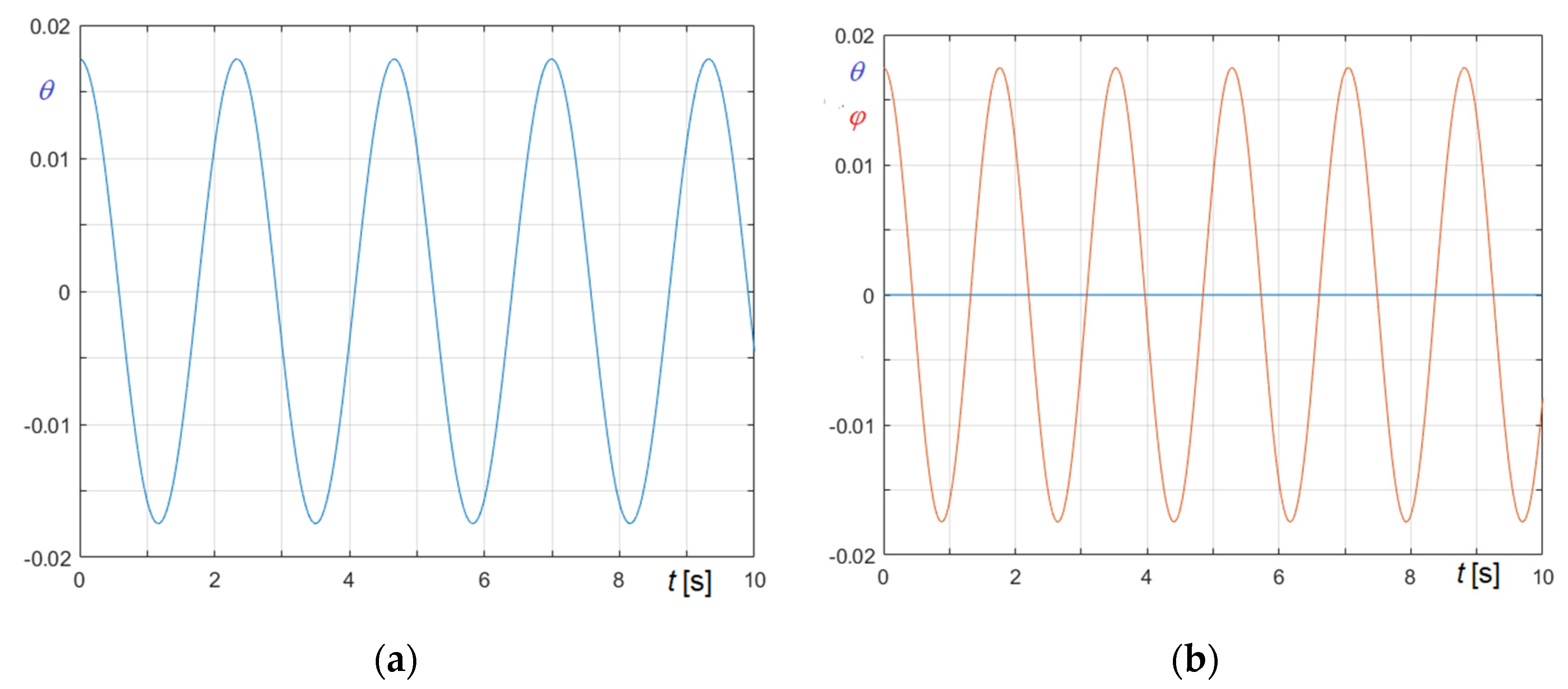
8.1.2. Case II Undamped Free Oscillations $\left({\mathsf{\theta }}_0=40°\right)$

Results regarding case II, undamped oscillations of the bell starting from ${\theta }_0=40°$, are reported in Figure 14a,b in terms of $\theta =\theta \left(t\right)$ and $\phi =\phi \left(t\right)$ curves, in Figure 14c,d in terms of $\phi -\dot{\phi }$ curves, and in Figure 14e,f in terms of $\theta -\dot{\theta }$ curves, in analogy with the criterion adopted for case I.

It must be underlined that in case II.b there are no impacts, while in case II.a, on average, impacts occur about every two oscillations. That results even more clearly from Figure 15a,b, which illustrates the time−angular acceleration curves $\ddot{\theta }=\ddot{\theta }\left(t\right)$ and $\ddot{\phi }=\ddot{\phi }\left(t\right)$ obtained in case II.b adopting $\Delta t=0.1 \mathrm{ms}$. In the figures, impacts obviously correspond to sudden variations, whose extents, recalling Equation (23) or (24), are inverse function of the adopted time step.

These remarks are further corroborated by

Table 7. Max amplitudes ${\theta }_1^{\ast }$, ${\theta }_5^{\ast }$, apparent periods $T_1^{\ast }$ and $T_5^{\ast }$ and apparent logarithmic decrements in Cases II.a and II.b.

	${\mathit{\theta }}_1^{\ast }$	${\mathit{\theta }}_5^{\ast }$	${\mathit{\delta }}_{\mathit{\theta }}^{\ast }$	${\mathit{T}}_1 \left[\mathit{s}\right]$	${\mathit{T}}_5 \left[\mathit{s}\right]$	${\mathit{\delta }}_{\mathit{T}}^{\ast }$
Case I.a	0.7066	0.7047	5.18·10−4	2.402	2.400	1.83·10−4
Case I.b	0.6981	0.6981	----	2.400	2.400	----

, evidencing that in case II.a part of energy is lost, while in case II.b, lacking any kind of dissipation, the energy is conserved.

The latter observation confirms that the proposed methods are symplectic integrators and that the energy drift is practically nil.

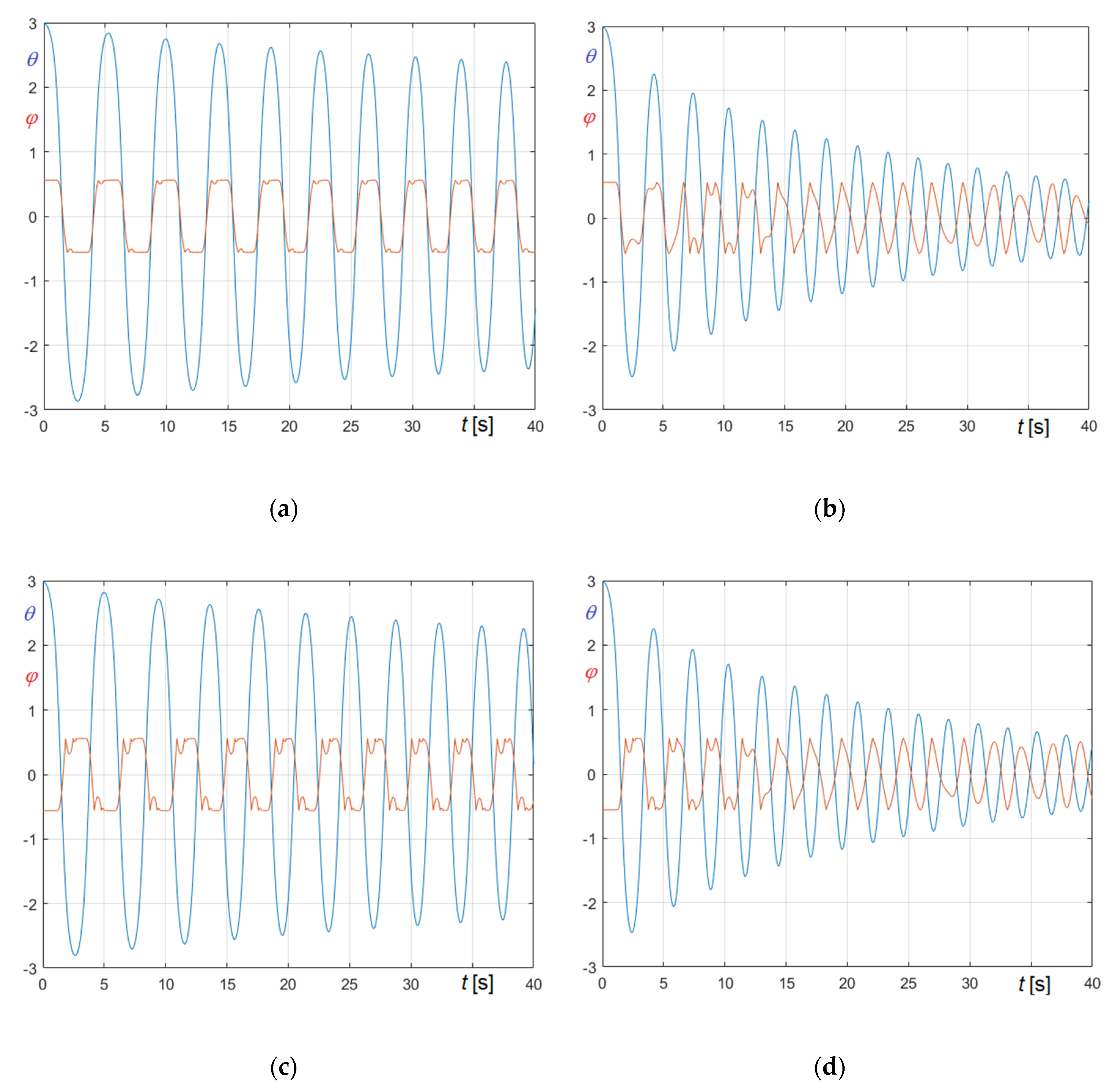
Recalling Equations (33) and (34), the radial accelerations at the clapper pivot $B^{\prime }$ and at the bell pivot $A$, including gravity acceleration, can be finally obtained as

$${\overrightarrow{a}}_{{rB}^{\prime }}=\left(\begin{array}{c}b {\left(\dot{\theta }+\dot{\phi }\right)}^2\sin \left(\theta +\phi \right)\\ \\ b {\left(\dot{\theta }+\dot{\phi }\right)}^2\cos \left(\theta +\phi \right)+g\end{array}\right) ,$$

(69)

$${\overrightarrow{a}}_{rA}=\frac{1}{M+m}\left(\begin{array}{c}\left(M a+m r\right) {\dot{\theta }}^2\sin \theta +m b {\left(\dot{\theta }+\dot{\phi }\right)}^2\sin \left(\theta +\phi -\alpha \right)\\ \\ \left(M a+m r\right) {\dot{\theta }}^2\cos \theta +m b {\left(\dot{\theta }+\dot{\phi }\right)}^2\cos \left(\theta +\phi -\alpha \right)+\left(M+m\right) g\end{array}\right) .$$

(70)

Referring again to case II.b, the resulting time histories of the dimensionless horizontal and vertical component of the radial accelerations in pivots $A$ and $B^{\prime }$ are illustrated in Figure 16. More precisely, Figure 16a,b refers to horizontal components $a_{rA,x}/g$ and $a_{r{B}^{\prime },x}/g$, while Figure 16c,d refers to vertical components $a_{rA,y}/g$ and $a_{r{B}^{\prime },y}/g$.

As expected, that amplitude does not induce significant excitation on the supports.

8.2. Viscous and Friction Damped Free Oscillations

Aiming to compare “equivalent” damping phenomena, case I.a has been studied considering viscous or friction damping as well. Preliminarily, the equivalence between viscous and friction damping has been assessed.

As known, the period, $T_d$, of viscous damped small free oscillations is constant over time; it depends only on the damping ratio $\zeta$ and on the period, $T$, of undamped oscillations, being independent on the exponentially decreasing amplitude of oscillations

$$T_d=\frac{T}{\sqrt{1-{\zeta }^2}}.$$

(71)

On the contrary, the apparent period of friction damped oscillations rigorously depends, besides on the friction coefficient, also on the amplitude of the oscillations; consequently, it varies over time, although slightly and the system generally does not retrieve the rest position. Given that the decay rate of friction damped oscillations is not exponential, their logarithmic decrement is variable, therefore the parameters of the equivalent viscous damping depend on the equivalence criterion.

Thanks to its simplicity, widely used procedures to determine the damping coefficient are based on the measurement of the period of damped oscillations or on the evaluation of the logarithmic decrement ${\delta }^{\ast }$.

The damping ratio $\zeta$ can be thus calculated using Equation (71) or by the formula:

$$\zeta ={\left[1+{\left(\frac{2 \pi }{{\delta }^{\ast }}\right)}^2\right]}^{-0.5}.$$

(72)

Following that procedure, the equivalence between friction and viscous damping has been established equalizing the logarithmic decrement of the viscous case and the apparent logarithmic decrement ${\delta }_{eq}^{\ast }$ of the friction case determined over five oscillations, using the first Equation (68), accordingly deducing damping ratios and damping coefficients. The amplitude of the first oscillation has been assumed, in turn, ${\theta }_0=5°$ or ${\phi }_0=5°$.

For the St. Mary’s tenor bell, assuming ${\mu }_b=0.02$ and $r_b=50 \mathrm{mm}$, at the bell pivot, and ${\mu }_c=0.04$ and $r_c=10 \mathrm{mm}$, at the clapper pivot, the equivalent damping ratios and the relative damping coefficient indicated in the last two columns of

Table 8. Friction parameters and 5° equivalent viscous damping parameters of St. Mary’s tenor bell.

	Pivot Radius [m]	Friction Coefficient	${\mathit{\delta }}_{\mathit{e}\mathit{q}}^{\ast }$	$\mathit{\zeta }$	$\overline{\mathit{c}} \left[\mathbf{m} {\mathbf{s}}^{-1}\right]$
Bell	0.05	0.02	8.077·10−2	1.285·10−2	9.354·10−2
Clapper	0.01	0.04	3.413·10−2	5.432·10−2	2.993·10−2

have been derived. As already said, the equivalence of the clapper has been derived assuming $r=0$.

The corresponding “equivalent” time histories of bell and clapper rotation are illustrated in Figure 17a,b, respectively: dashed lines refer to friction cases, and continuous lines to viscous cases.

Looking at the figures, it is evident that, although first oscillations of friction and viscous curves are nearly coincident, over time friction decay tends to prevail.

Comparison of Large Damped Free Oscillations in Case I $\left({\mathsf{\theta }}_0=171°\right)$

Cases I.a and I.b have been studied also in damped conditions, adopting the damping equivalent parameters previously determined (Table 8), assuming the initial values given by Equations (64) and (65).

The results are compared in Figure 18 in terms of time histories of rotations, in Figure 19 in terms of $\dot{\theta }-\theta$ curves, and in Figure 20 in terms $\dot{\phi }-\phi$ curves.

Figure 18a,b shows the time histories of bell and clapper rotations derived in case I.a—bell ringing right—considering friction damping and viscous damping, respectively; Figure 18c,d refer to the corresponding situations in case I.b−bell ringing wrong.

Figure 19a,b compares $\dot{\theta }-\theta$ curves in case I.a e I.b, respectively, while Figure 19c,d compares the corresponding curves $\dot{\phi }-\phi$. In these diagrams, curves pertaining to friction damping are in blue and curves pertaining to “5° equivalent” viscous damping are in red.

The diagrams demonstrate that equivalent viscous damping coefficients determined considering small oscillations cannot be adopted for large oscillations. In fact, the comparison of diagrams in Figure 18 and Figure 19 is a crystal-clear evidence that amplitude and period decrease more quickly for “5° equivalent” viscous damped oscillations than for friction damped oscillations.

The reason for the latter remark is that, as soon as the initial amplitude of the oscillations increases, viscous dissipation increases much more rapidly than friction dissipation. The observation can be further corroborated comparing the energy dissipation caused by friction or by viscosity in a group of cycles or in a given time interval.

Since energy dissipation is nothing else than the work done by the corresponding dissipative force, its calculation is not particularly difficult.

The energy dissipated by friction damping and the energy dissipated by “5° equivalent” viscous damping are compared in the diagrams of Figure 20 and Figure 21a.

In Figure 20 the dissipated energies $E_{dis}$ are plotted as a function of the bell rotation, $\theta$, cycle by cycle: Figure 20a refers to the small oscillation case considered to assess the equivalence, Figure 20b to the case I.a.

To facilitate the reading, curves in Figure 20b are parameterized considering different time intervals: the dashed magenta curve is the energy dissipated by friction in the time interval $0-25 \mathrm{s}$, while the solid blue line is the energy dissipated by “5° equivalent” viscosity in the time interval $0-6 \mathrm{s}$. Finally, the $E_{dis}-t$ curves obtained for case I.a are compared in Figure 21a, in which solid line refers to “5° equivalent” viscosity and dashed line to friction.

Figure 20a clearly shows that, as expected, for 5° oscillations the energy dissipations due to friction or equivalent viscosity practically coincide, but Figure 20b and Figure 21a underline that using “5° equivalent” viscosity leads to huge overestimations of the dissipated energy. That confirms that the equivalence parameters between friction and viscous dissipation is sensibly dependent on the initial amplitude. This aspect is not surprising since the energy dissipation due to friction depends, apart from the oscillation amplitude, on the increase of the friction forces due to the increase of radial forces, while the energy dissipation due to viscosity depends, besides the oscillation amplitude, on the angular velocity.

Owing the fact that the mean modulus of the radial acceleration at the pivot $A$, which is $\overline{\left|a_{rA}\right|}\approx g$ for ${\theta }_o=5°$ oscillations, becomes $\overline{\left|a_{rA}\right|}\approx 2.2 g$ for ${\theta }_o=171°$ oscillations, and that the mean angular velocity, which is $\overline{\dot{\theta }}\approx 0.15 {\mathrm{s}}^{-1}$ for ${\theta }_o=5°$ oscillations, becomes $\overline{\dot{\theta }}\approx 2.5 {\mathrm{s}}^{-1}$ for ${\theta }_o=171°$ oscillations, the energy dissipations in ${\theta }_o=171°$ oscillations can be roughly estimated, starting from the dissipation evaluated considering ${\theta }_o=5°$ oscillations. As the mean value of the dissipated energy for ${\theta }_o=5°$ oscillations is around ${\overline{E}}_{dis}\left(5°\right)\approx 4 \mathrm{J}/\mathrm{cycle}$ (Figure 20a), the dissipation caused by friction in ${\theta }_o=171°$ oscillations, which is approximately ${\overline{E}}_{dis,f}\left(171°\right)\approx 42.234\approx 300 \mathrm{J}/\mathrm{cycle}$, results sensibly smaller than the energy dissipated by “5° equivalent” viscosity, which is around ${\overline{E}}_{dis,v}\left(171°\right)\approx 41634\approx 2200 \mathrm{J}/\mathrm{cycle}.$ It must be remarked that these values, although roughly estimated, satisfactorily fit the calculated values for the first cycles (Figure 21a).

To conclude the analysis, the “171° equivalent” viscous damping parameters have also been determined, reported in

Table 9. Friction and 171° equivalent viscous damping parameters of St. Mary’s tenor bell.

	Pivot Radius [m]	Friction Coefficient	$\mathit{\zeta }$	$\overline{\mathit{c}} \left[\mathit{m} {\mathit{s}}^{-1}\right]$
Bell	0.05	0.02	0.97·10−3	7.051·10−3
Clapper	0.01	0.04	0.50·10−3	2.750·10−3

. These values, which are one order of magnitude lower than the ones determined for small oscillations (Table 8), lead to the time−dissipated energy curve illustrated in Figure 21b (solid line), substantially coinciding with the dashed curve regarding the friction case.

In addition, the entity of the dissipative forces can play an important role in discriminating the aptitude of the bell to ring right or wrong, as demonstrated by the St. Mary’s tenor bell behavior when large free oscillations are considered. In fact:

• on the one hand, as long as dissipative forces are low, over the time the bell tends to maintain the initial ringing state (right or wrong) (see Figure 18a,c),
• on the other, if dissipative forces increase, the bell tends to switch, independently on the initial state, into a ringing wrong state, in which each cycle is characterized by a single instantaneous impact (see Figure 18b,d).

8.3. Time Histories of Excitations at the Pivots in Case of Large Oscillations $\left({\theta }_0=171°\right)$

Adopting the approach already described in Section 8.1.2. for case II—undamped free oscillations with ${\mathsf{\theta }}_0=40°$, the time histories of the excitations at the bell and clapper pivots in case of full circle oscillations $\left({\theta }_0=171°\right)$ have also been determined, considering undamped and friction damped oscillations. Recalling that the “equivalent” viscous damping case, whose parameters accord with Table 9, leads to outcomes practically coinciding with the ones obtained for friction damping, this case has not been explicitly considered.

The time histories of the accelerations are compared in Figure 22, where solid lines refer to the undamped situation and dashed lines to the damped situation.

In analogy with Figure 16, Figure 22a,b refers to horizontal components $a_{rA,x}/g$ and $a_{r{B}^{\prime },x}/g$, while Figure 22c,d refers to vertical components $a_{rA,y}/g$ and $a_{r{B}^{\prime },y}/g$. The diagrams show that the apparent period of damped large oscillations decreases over time, as a consequence of the reduction of the amplitude of the oscillations, which largely compensates the small increase due to the (low) damping considered in the present case. Obviously, this aspect is particularly relevant not only for the assessment of the bell behavior but also for the evaluation of the actions to be considered dealing with bell-structure interactions.

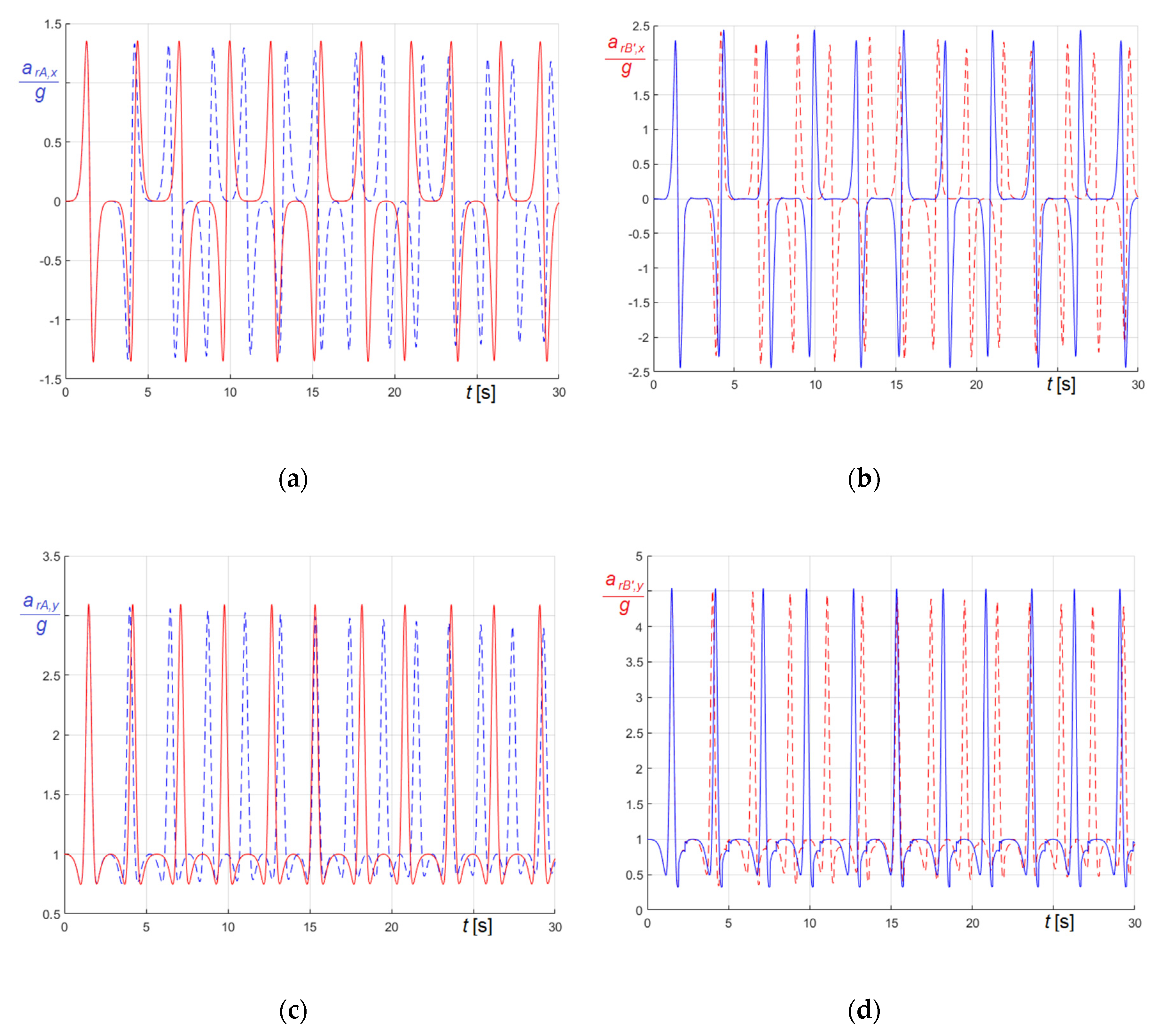
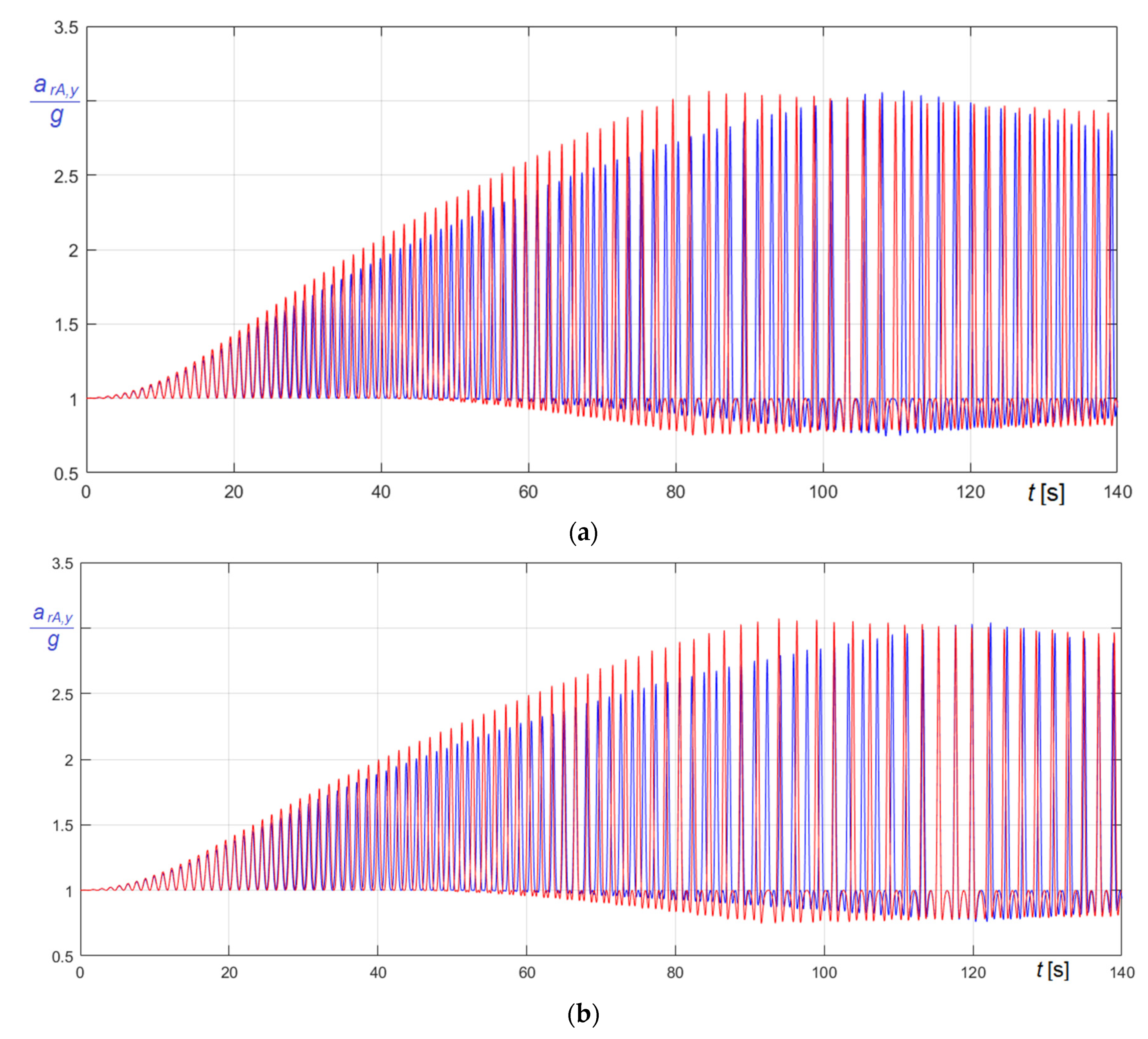
8.4. Synchronized Resonant Forced Oscillations of the Bell in Transient Phase

As known, manual excitation of a ringing bell in the starting phase is a typical example of resonance, where the forcing frequency is suitably tuned by the bell player in such a way that it is constantly synchronized with the natural frequency of the bell, which decreases as the oscillation amplitude increases. From the mathematical point of view, modelling this operation is not trivial, due to the complexity of the relationship between the natural frequency of the oscillations, their amplitude, the damping parameters, and their variations over time. For that reason, the study of this relevant transient phase is often disregarded or drastically simplified, for example considering easy to handle periodic forcing functions.

Dealing with forced oscillations, external forces are usually modeled by means of cosinusoidal functions of the time, so opening the door for easier analytical treatment. A similar approach is often adopted also in numerical integration of the equations of motion, especially when the solution is achieved via standard built-in numerical algorithms. Obviously, if the problem involves resonance aspects, the frequency of the forcing cosinusoidal function should be continuously modified to catch the actual natural frequency of the system, as a function of the oscillation amplitude. That approach is often worthless since it requires systematic human intervention to proceed with the solution. A common line of action is to consider forcing functions characterized by fixed frequency, suitably chosen in the range of natural frequencies associated with the expected range of oscillation amplitudes. Difficulties further increase considering external excitations described by arbitrary functions of the time, like, for example, the stepwise constant real excitations applied by bell ringers or by linear or rotating motors.

The proposed algorithms overcome all these issues. Really, they are able to successfully manage quite arbitrary excitations, $M_e\left(\theta ,t\right)$ and $m_e\left(\phi ,t\right)$, of bell and clapper, also in case their dependence on time is not explicit. That important original feature easily allows to automatically synchronize the excitation with the varying instantaneous natural frequency of the system, reproducing persistently resonant conditions and, consequently, minimizing the peaks of the excitation.

A possible workaround is considering torques explicitly depending only on the rotations, so that the dependence on $t$ is implicitly expressed through $\theta =\theta \left(t\right)$ and $\dot{\theta }=\dot{\theta }\left(t\right)$ or $\phi =\phi \left(t\right)$ and $\dot{\phi }=\dot{\phi }\left(t\right)$. It is worthwhile to remark that, even if the focus of the study is bell excitation, the approach is much more general, and it is not subject to special limitations.

Moreover, in defining the forcing function it should considered that, depending on the arrangement, external torque can be unidirectional or bidirectional, like in the case handstroke and backstroke consent to swing the bell through a full circle.

To assess the potentiality of the method, it has been studied the transient situation corresponding to the time interval needed to achieve the bell working position, starting from the rest condition. In the simulation, once achieved the bell working position, ${\theta }_{max}\approx 171°$, the excitation has been switched off, so subsequently leaving the bell free to oscillate.

Four cases have been analyzed, characterized by two different forcing functions and by undamped or damped oscillations. In all cases, the following initial conditions have been assumed:

$$\theta \left(0\right)=2°; \dot{\theta }\left(0\right)=0; \phi \left(0\right)=-2°; \dot{\phi }\left(0\right)=0 ,$$

(73)

which correspond to an initial small rotation of the bell, with the clapper in vertical position.

Aiming to reproduce a manual excitation, it has been adopted a piecewise-constant bidirectional forcing function, which is the more realistic one:

$$M_{e1}\left(\theta ,\dot{\theta }\right)=\{\begin{array}{c}250 \mathrm{sgn} \dot{\theta } Nm \mathrm{if}-\frac{\pi }{4}\le \theta \le \frac{\pi }{4}\\ \\ 0 \mathrm{if} \theta \langle -\frac{\pi }{4} \vee \theta \rangle \frac{\pi }{4}\end{array},$$

(74)

or a truncated sinusoidal bidirectional forcing function:

$$M_{e2}\left(\theta ,\dot{\theta }\right)=\{\begin{array}{c}250 \mathrm{sgn} \dot{\theta }\cos \theta Nm \mathrm{if}-\frac{\pi }{4}\le \theta \le \frac{\pi }{4}\\ \\ 0 \mathrm{if} \theta \langle -\frac{\pi }{4} \vee \theta \rangle \frac{\pi }{4} \end{array}.$$

(75)

It must be remarked that the peak modulus of $M_{e1}$ and $M_{e2}$, $250 \mathrm{Nm}$, matching the torque easily exerted by a person, is significantly smaller than the peak of the torque needed to lift statically the St. Mary’s tenor bell in the upward position, $M_{max}\approx 10 \mathrm{kNm}$.

Since “equivalent” viscous parameters strongly depend on the amplitude of the oscillations, the damped case refers to friction damping. Friction coefficients and pivot radii are those already recalled in Table 8 and Table 9, leading to very low level of damping, corresponding to a damping ratio $\zeta \approx 0.1\%$.

Relevant curves obtained in the undamped and in the friction damped case are compared in Figure 23, Figure 24 and Figure 25. In the figures, panel (a) refers to $M_{e1}$ (Equation (74)), and panel (b) to $M_{e2}$ (Equation (75)); curves referring to undamped case are generally in blue and curves referring to damped case are generally in red, except $\phi -t$ curves in Figure 23, whose colors are opposites.

Looking at the time histories of the rotations of bell and clapper (Figure 23), it results that:

• in the undamped case, the time needed to reach the maximum amplitude, $t_d$, i.e., the time during which the bell is driven, is $t_d\approx 83 \mathrm{s}$, when the forcing function is $M_{e1}$, increasing to $t_d\approx 93 \mathrm{s}$, when the forcing function is $M_{e2}$,
• in the friction damped case, the time needed to reach the maximum amplitude is $t_d\approx 110 \mathrm{s}$, when the forcing function is $M_{e1}$, increasing to $t_d\approx 121 \mathrm{s}$, when the forcing function is $M_{e2}$,
• also considering the transient phase, and without stopping it in the upward position before the free oscillation phase, the bell tends to ring wrong in all considered cases.

Further information can be derived from the time histories of the horizontal and of the vertical component of the acceleration at the bell pivot $A$, illustrated in Figure 24 and Figure 25, respectively.

Considering forced oscillations, the comparison of the diagrams obviously confirms that the number of oscillations needed to reach a given state in the transient phase is bigger in damped conditions than in undamped conditions.

Anyhow, it is interesting to remark that the amplitude and the period of these forced damped oscillations are generally smaller than those pertaining to forced undamped oscillations, even if, clearly, as already anticipated, the apparent period of a given large oscillation is higher in damped condition.

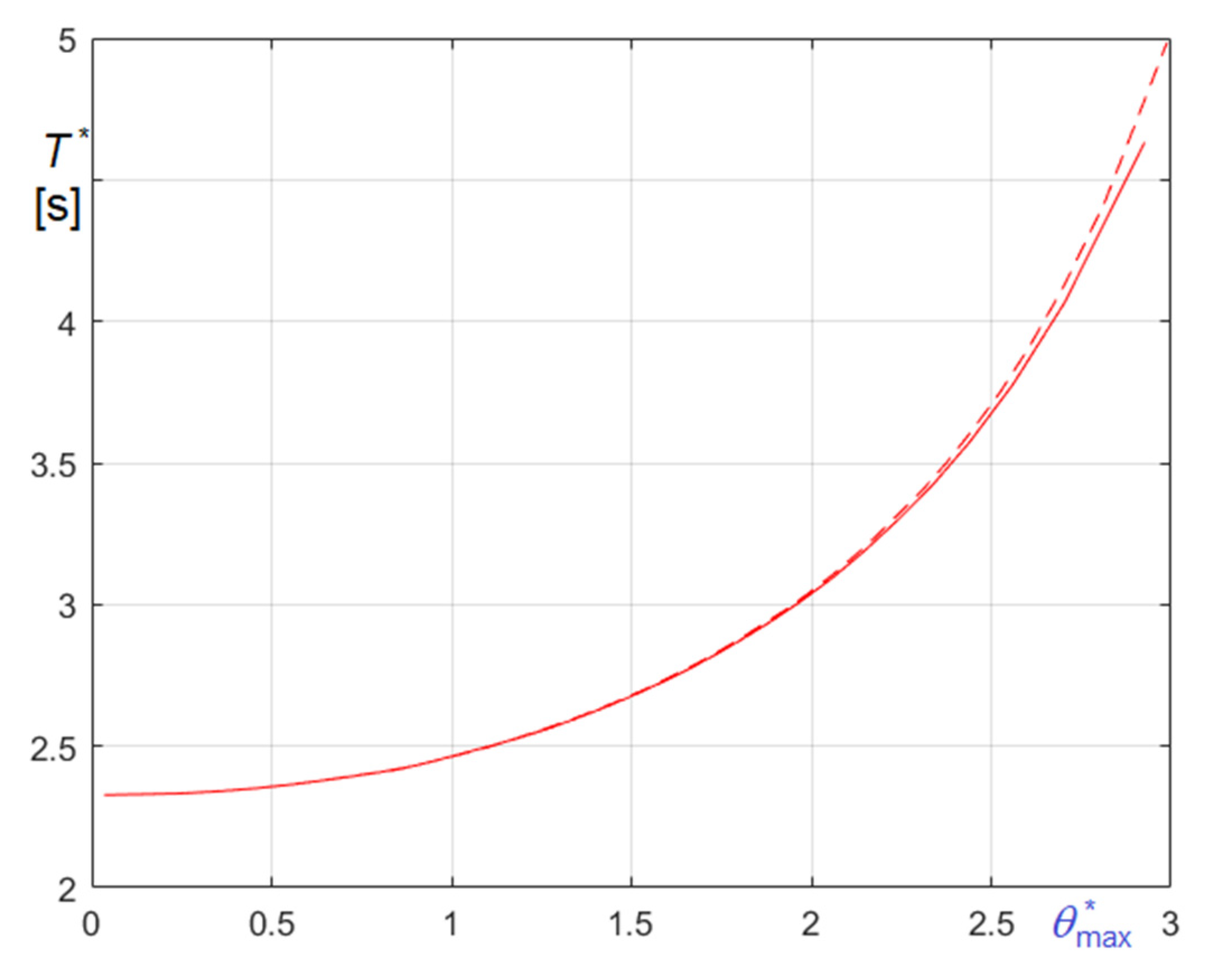
The latter observation is diagrammatically illustrated in Figure 26, where, referring to the present case study, the apparent periods $T^{\ast }$ of the forced resonant oscillations are plotted as a function of the maximum amplitude of the oscillations themselves ${\theta }_{\max }^{\ast }$. In the diagram, dashed line represents the damped case, solid line the undamped case. Evidently, due to the low damping ratio characterizing the case study, the increase of the period due to damping is significant only when the oscillation amplitude is large.

Finally, adopting a representation in line with that adopted for Figure 23, Figure 24 and Figure 25, in Figure 27 they are illustrated, as functions of the time, the resonant forcing functions resulting, in the considered cases, in damped and undamped conditions.

Obviously, Figure 27a refers to $M_{e1}$ (Equation (74)), Figure 27b to $M_{e2}$ (Equation (75)). The graphs clearly demonstrate that the period of the forcing frequency is automatically tuned on the period of the system, so certifying the capability of the proposed approach to simulate also constantly resonant excitations.

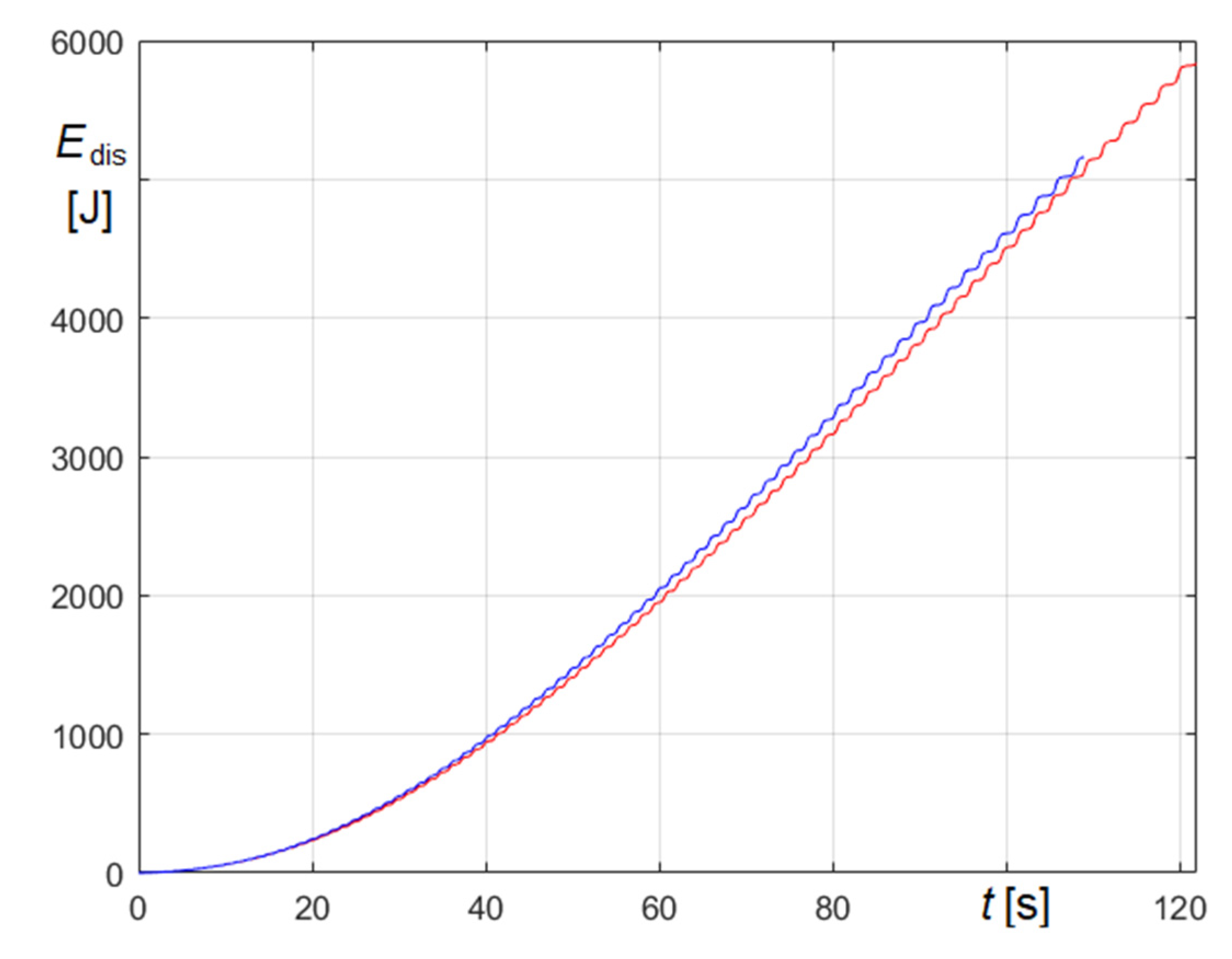
To complete the case study, the energy dissipated in the transient phase of forced damped oscillations are represented as a function of the time in Figure 28. In the figure, the blue line refers to $M_{e1}$ and the red line to $M_{e2}$. The total energy dissipated to attain the maximum amplitude results $E_{dis}\approx 5.15 \mathrm{kJ}$, if the forcing function is $M_{e1}$, increasing to $E_{dis}\approx 5.85 \mathrm{kJ}$, if the forcing function is $M_{e2}$, so indicating that, as expected, $M_{e1}$ excitation is more efficient.

Evidently, the duration of the transient phase depends on shape and intensity of the forcing excitation, as well as on the initial conditions, but the proposed algorithms are not sensitive on it. In fact, as already remarked at the end of Section 6, the procedure can be repeated as many times as necessary, duly modifying the initial condition, until the wanted final condition is achieved.

9. Conclusions

Study of swinging bells involves topical arguments of structural and mechanical engineering as well as sound and acoustic engineering.

The research focuses, first, on the system of two nonlinear second order ODEs governing the problem. That system is derived under very general hypotheses, considering viscous damping, friction damping, and arbitrary excitations. Dissipative forces are treated like external forces interpreting the equation of motion of bell and clapper as dynamic equilibrium equations, in the spirit of Newtonian mechanics.

In the study, besides viscous forces proportional to the angular velocities, friction forces at the bell and clapper pivots are introduced as well. In that novel perspective, friction forces, commonly disregarded in the traditional approach, are realistically expressed as a function of the time dependent reactive radial forces at the pivots.

Clapper strokes are modelled as instantaneous impacts, resorting to the kinematic definition of the coefficient of restitution, which allows a synthetic, and experimentally measurable, quantification of the complex interdependency between the relevant parameters governing the impact. The suitable application of the law of conservation of the angular momentum provides the bell and clapper angular velocities at the end of the impact, which can be easily modified to consider also the acoustic energy leaving the system. Moreover, to preserve the physical coherence avoiding paradoxical results, the upper bound of the coefficient of restitution, corresponding to perfectly elastic impact, is suitably derived.

In the relevant literature about classical bell dynamics, the focus is alternatively concentrated on the bell-clapper interactions or on the bell-tower excitation. Whatever the problem, analytical solutions are available in a limited number of cases, therefore the governing ODEs are usually solved using numerical methods. The most frequently used numerical approaches rely on standard built-in algorithms, available in advanced software packages. Since adoption of these general algorithms is subject to some restrictions and often requires some additional manipulation of the equations, especially regarding the forcing functions, the significance of the outcomes derived in that way is limited. Moreover, the piecewise-defined structure of the solution makes the use of these classical methods even more complex.

In the paper an innovative procedure to solve the equations of motions of bell and clapper is discussed.

The novelty of the proposed method, which is described in Section 6, is an original numerical explicit-implicit predictor-corrector integration scheme with constant time step, implemented in two different slightly different versions, depending on the correction phase regards only the rotations or the angular velocities and the angular accelerations as well. The implementation is such that each time the clapper strikes the bell a new “piece” of the solution is automatically initialized, consequently user interventions in the elaboration phase are not necessary.

In addition, the structure of the algorithm allows to analyze arbitrarily long transient and stationary time intervals, until the required final situation is achieved, provided that the total time to be analyzed is divided in suitable subintervals. Evidently, the duration of each subinterval should be chosen according the available physical memory of the computer hardware, while the initial conditions of the system in each subinterval are obtained duly recalling the final conditions of the system at the end of the preceding subinterval.

These extremely fast and effective algorithms, which have been validated in Section 7 reproducing relevant theoretical, numerical, and experimental outcomes, allow one to successfully handle, independently on the oscillation amplitude: undamped oscillations; friction and viscosity damped oscillations; free oscillations; forced oscillations; transient and stationary phases, and are also suitable to solve stiff equations.

The method has been applied in Section 8 to study the oscillations of a relevant bell, the Great St. Mary’s old tenor bell in Cambridge, hypothesizing several distinct operational conditions, also highlighting that the definition of damping equivalence requires nontrivial considerations.

The critical examination of the outcomes of the analyses demonstrates the potentialities of the method highlighting some original key issues, like its capability to handle arbitrary forcing functions.

A particularly significant and pioneering feature of the algorithms is their ability both to manage and to define “resonant” forcing functions, continuously tuned on the actual frequency of the oscillation, which depends on the amplitude of the oscillation itself. Outstanding examples of resonant forcing functions are, for example, the excitations that bell ringers apply on manually driven bells.

It must be stressed that the approach is absolutely general and can be applied independently on the adopted ringing style; as well as on dimensions, shape, and mechanical properties of bell and clapper.

Further refinements, especially regarding other sources of dissipation; linear and nonlinear external elastic restraints; and interaction with the supporting structures can be envisaged, which will be the subject of future studies.