Operational Performance and Degradation of PV Systems Consisting of Six Technologies in Three Climates


Abstract
1. Introduction
- -
- Reading in available input data;
- -
- Data filtering;
- -
- Selection of performance metric;
- -
- Possible correction and data aggregation;
- -
- Application of the statistical method to calculate the final PLR.
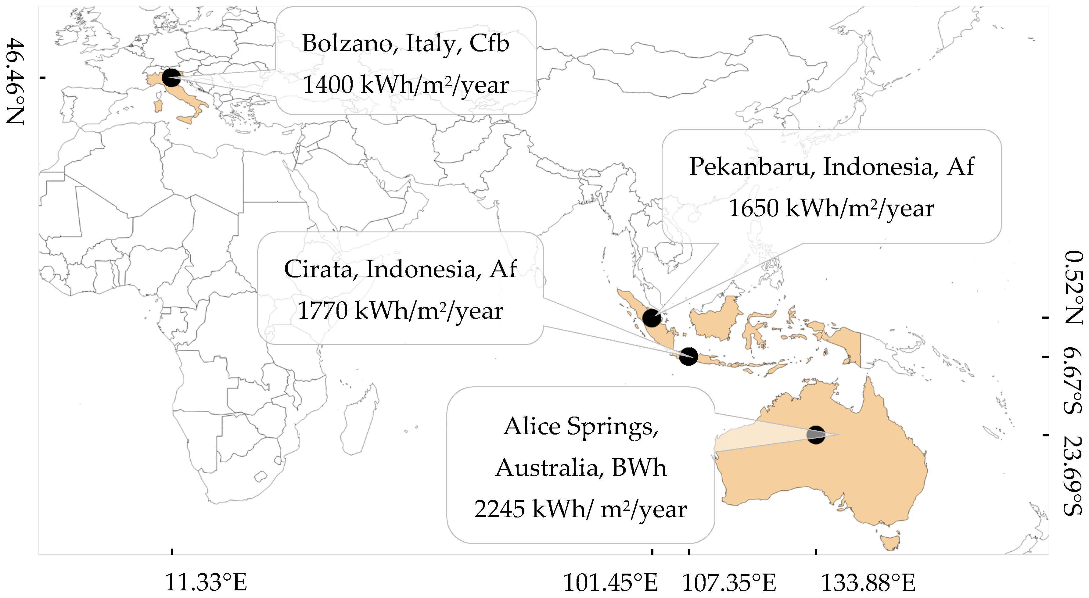
2. Experimental Set-up
3. Methods
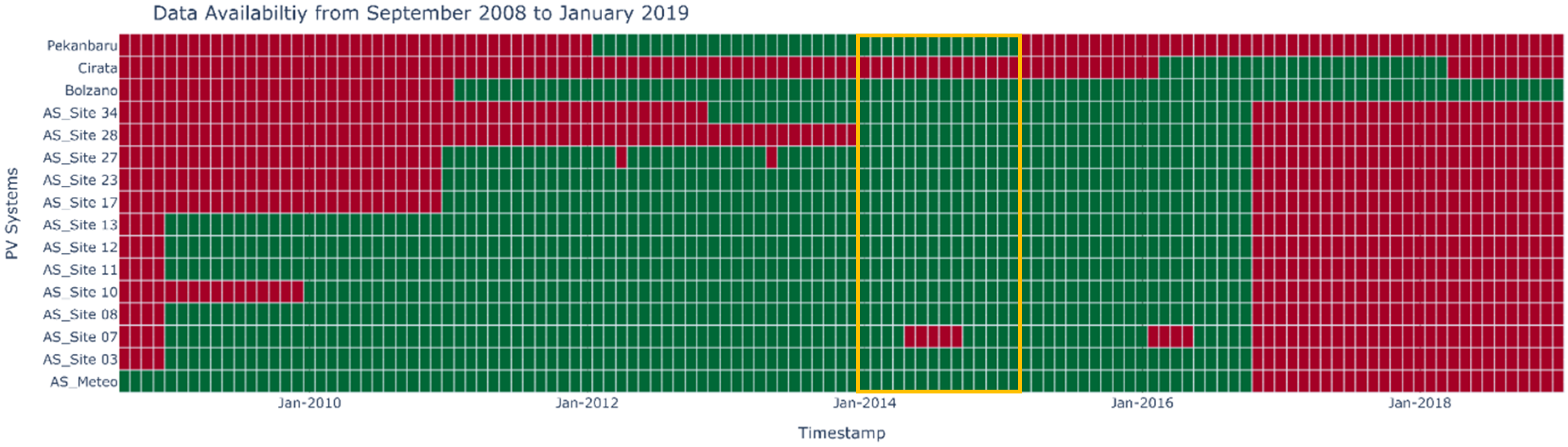
3.1. Data Preparation
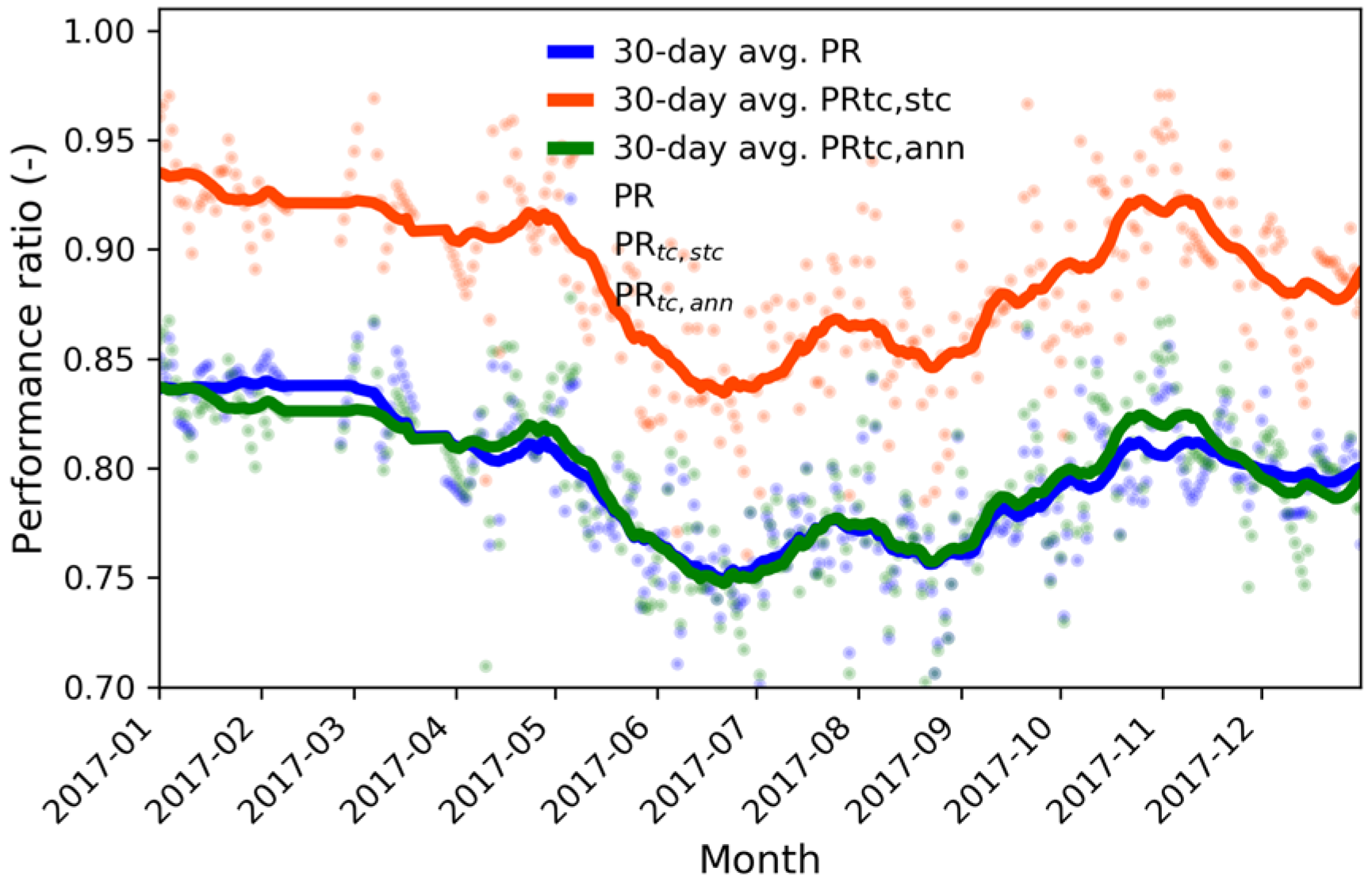
3.2. Calculation of the Performance Ratio
3.3. Calculation of the Performance Loss Rate Using Linear Regression and STL
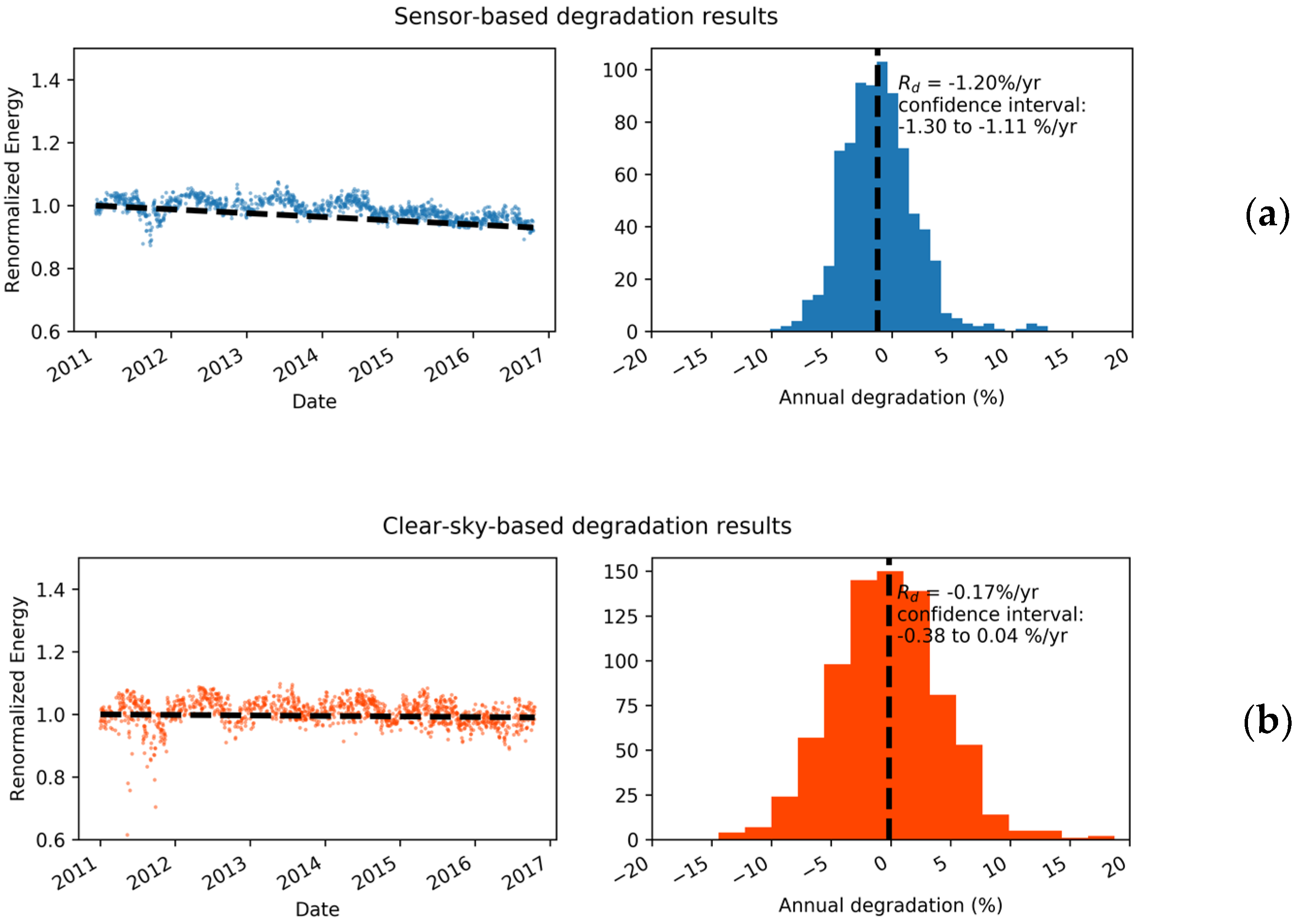
3.4. Calculation of the Performance Loss Rate Using the YoY Approach
4. Results and Discussion
4.1. Performance Ratio
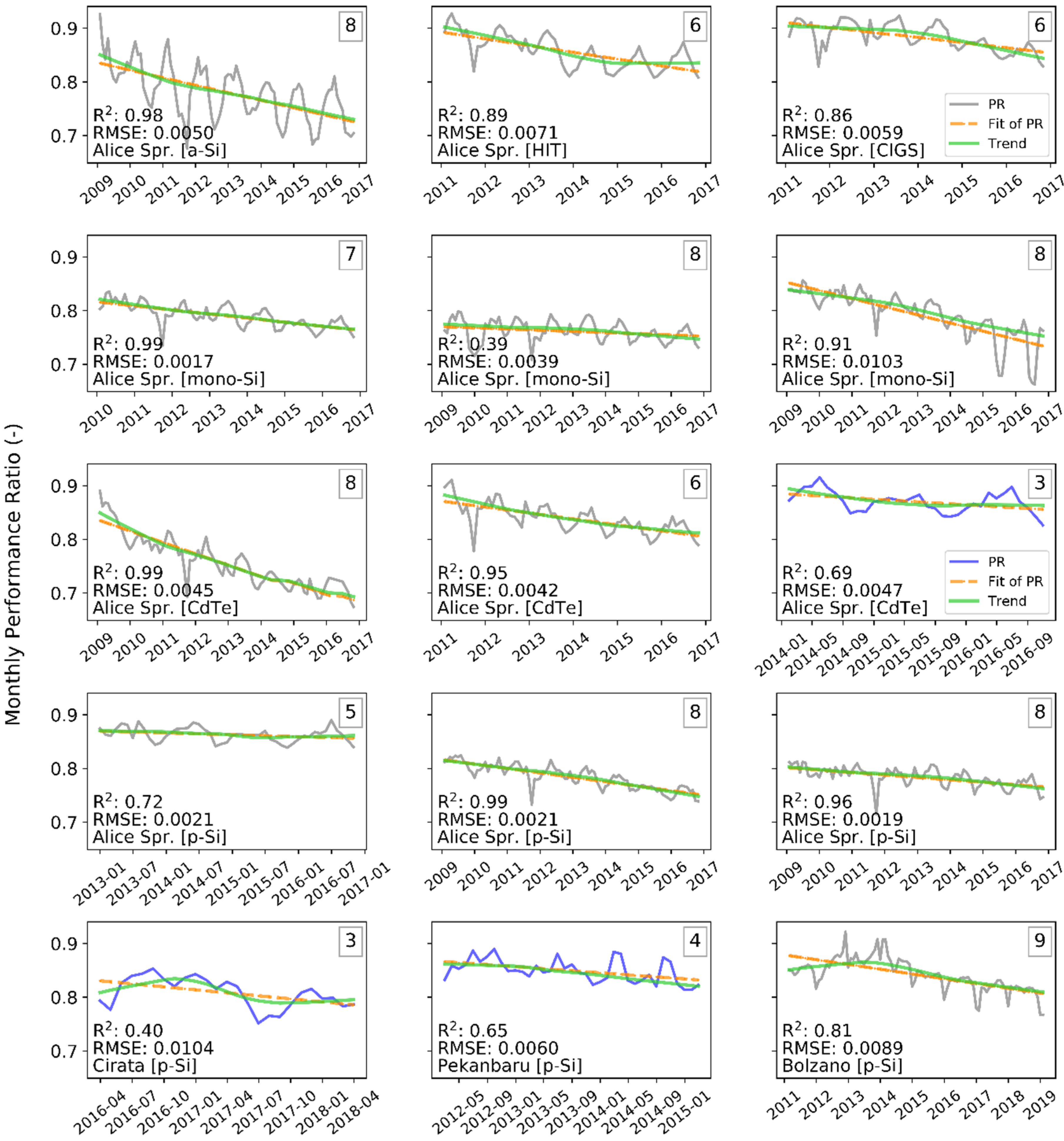
4.2. Performance Loss Rate Calculation Using LR and STL
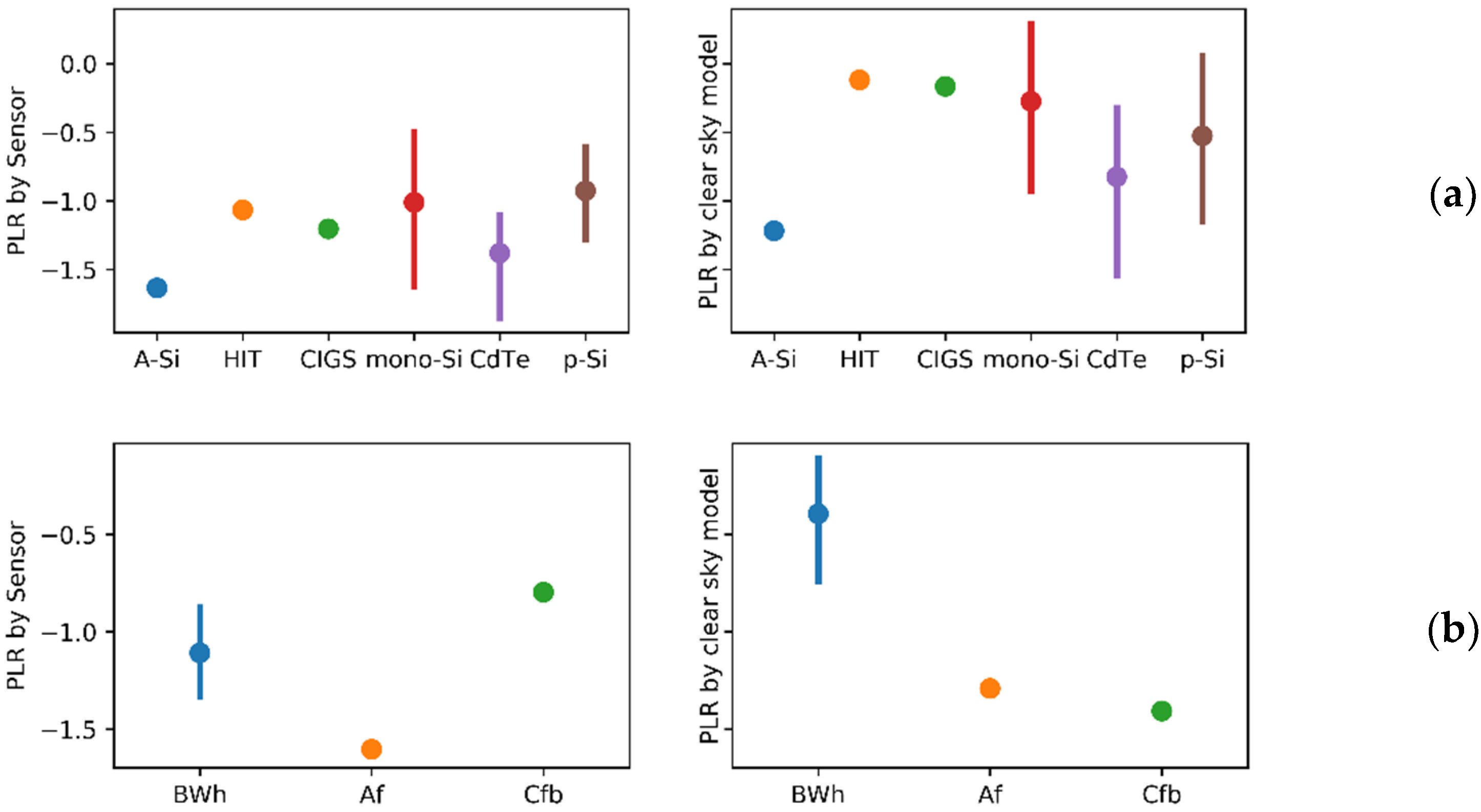
4.3. Comparison of PLR Values Using STL and YoY
5. Conclusions
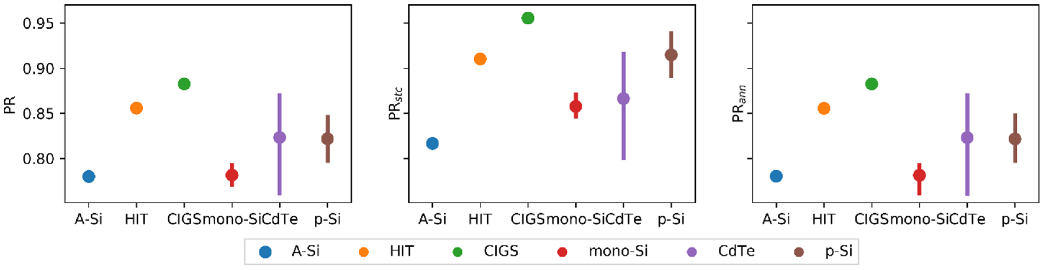
- The annual-averaged temperature-corrected performance ratio, PRann., with an average value of all systems from each technology. The CIGS system performed best with an average PR value of 0.88 ± 0.04. The least performing technology was the a-Si PV systems, with an average PR value of 0.78 ± 0.05. The p-Si systems in climate Cfb of Italy had a higher average PR of 0.84 than those operating in climates BWh (Australia) and Af (Indonesia), with the same value of 0.81.
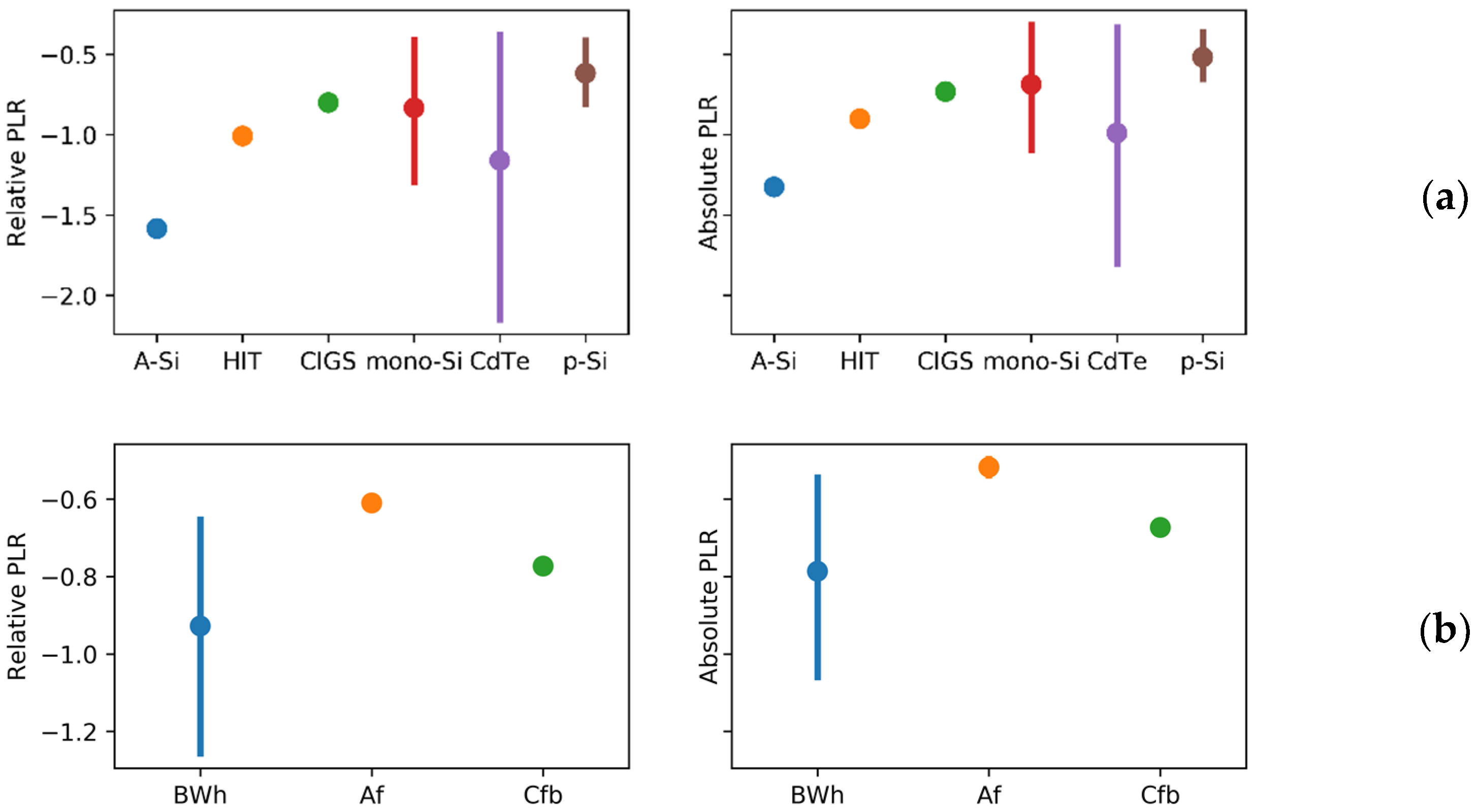
- Performance loss rates based on the STL approach. For almost all systems, the use of STL for the calculation of PLR is helpful, especially if monitoring data of high quality was not available. The p-Si systems show the lowest PLR among the technologies with an average PLR value of −0.6%/year. The strongest performance loss was experienced by a-Si modules at −1.58%/year.
Author Contributions
Funding
Acknowledgments
Conflicts of Interest
Appendix A

| No. | City | Climate | Technology | PR | PRstc. | PRann. | PLR (%/year) YoY | PLR (%/year) STL | |
|---|---|---|---|---|---|---|---|---|---|
| Sensor | Clear Sky | Relative | |||||||
| 1 | Alice Springs | BWh | a-Si | 0.78 ± 0.05 | 0.82 ± 0.05 | 0.78 ± 0.05 | −1.63 | −1.22 | −1.58 |
| 2 | Alice Springs | BWh | HIT | 0.86 ± 0.04 | 0.91 ± 0.03 | 0.86 ± 0.03 | −1.07 | −0.12 | −1.01 |
| 3 | Alice Springs | BWh | CIGS | 0.88 ± 0.04 | 0.96 ± 0.03 | 0.88 ± 0.03 | −1.20 | −0.17 | −0.80 |
| 4 | Alice Springs | BWh | mono-Si | 0.79 ± 0.03 | 0.86 ± 0.02 | 0.79 ± 0.02 | −0.91 | −0.19 | −0.80 |
| 5 | Alice Springs | BWh | mono-Si | 0.76 ± 0.04 | 0.85 ± 0.02 | 0.76 ± 0.02 | −0.50 | +0.29 | −0.41 |
| 6 | Alice Springs | BWh | mono-Si | 0.79 ± 0.05 | 0.87 ± 0.05 | 0.79 ± 0.04 | −1.62 | −0.93 | −1.30 |
| 7 | Alice Springs | BWh | CdTe | 0.76 ± 0.05 | 0.80 ± 0.05 | 0.76 ± 0.05 | −1.85 | −1.55 | −2.20 |
| 8 | Alice Springs | BWh | CdTe | 0.84 ± 0.03 | 0.88 ± 0.03 | 0.84 ± 0.03 | −1.10 | −0.32 | −0.95 |
| 9 | Alice Springs | BWh | CdTe | 0.87 ± 0.03 | 0.92 ± 0.02 | 0.87 ± 0.02 | −1.19 | −0.60 | −0.38 |
| 10 | Alice Springs | BWh | p-Si | 0.86 ± 0.03 | 0.95 ± 0.01 | 0.86 ± 0.01 | −0.47 | +0.33 | −0.19 |
| 11 | Alice Springs | BWh | p-Si | 0.78 ± 0.04 | 0.94 ± 0.03 | 0.78 ± 0.02 | −1.12 | −0.36 | −0.97 |
| 12 | Alice Springs | BWh | p-Si | 0.78 ± 0.03 | 0.87 ± 0.02 | 0.78 ± 0.02 | −0.64 | +0.09 | −0.56 |
| 13 | Cirata | Af | p-Si | 0.81 ± 0.03 | 0.90 ± 0.03 | 0.81 ± 0.03 | n.a | n.a. | −0.60 |
| 14 | Pekanbaru | Af | p-Si | 0.85 ± 0.02 | 0.93 ± 0.02 | 0.85 ± 0.02 | −1.60 | −1.29 | −0.62 |
| 15 | Bolzano | Cfb | p-Si | 0.84 ± 0.04 | 0.89 ± 0.03 | 0.84 ± 0.03 | −0.80 | −1.41 | −0.77 |
References
- Ingenhoven, P.; Belluardo, G.; Moser, D. Comparison of statistical and deterministic smoothing methods to reduce the uncertainty of performance loss rate estimates. IEEE J. Photovolt. 2018, 8, 224–232. [Google Scholar] [CrossRef]
- Fouad, M.M.; Shihata, L.A.; Morgan, E.S.I. An integrated review of factors influencing the performance of photovoltaic panels. Renew. Sustain. Energy Rev. 2017, 80, 1499–1511. [Google Scholar] [CrossRef]
- De Graaf, L.E.; Van Der Weiden, T.C.J. Characteristics and performance of a PV-system consisting of 20 AC-modules. In Proceedings of the Conference Record of the IEEE Photovoltaic Specialists Conference, Waikoloa, HI, USA, 5–9 December 1994; pp. 921–924. [Google Scholar]
- Fraunhofer ISE. Photovoltaics Report 2019; Fraunhofer Institute for Solar Energy Systems ISE: Freiburg im Breisgau, Germany, 2019. [Google Scholar]
- Jordan, D.C.; Sarah, R. Kurtz Photovoltaic degradation rates—An Analytical Review. Prog. Photovolt. Res. Appl. 2013, 21, 12–29. [Google Scholar] [CrossRef]
- Ingenhoven, P.; Belluardo, G.; Makrides, G.; Georghiou, G.E.; Rodden, P.; Frearson, L.; Herteleer, B.; Bertani, D.; Moser, D. Analysis of Photovoltaic Performance Loss Rates of Six Module Types in Five Geographical Locations. IEEE J. Photovolt. 2019, 9, 1091–1096. [Google Scholar] [CrossRef]
- Jordan, D.C.; Deline, C.; Kurtz, S.R.; Kimball, G.M.; Anderson, M. Robust PV Degradation Methodology and Application. IEEE J. Photovolt. 2018, 8, 525–531. [Google Scholar] [CrossRef]
- Jordan, D.C.; Kurtz, S.R.; VanSant, K.; Newmiller, J. Compendium of photovoltaic degradation rates. Prog. Photovolt. 2016, 24, 978–989. [Google Scholar] [CrossRef]
- Makrides, G.; Zinsser, B.; Schubert, M.; Georghiou, G.E. Performance loss rate of twelve photovoltaic technologies under field conditions using statistical techniques. Sol. Energy 2014, 103, 28–42. [Google Scholar] [CrossRef]
- Larrivee, J. An Analysis of Degradation Rates of PV Power Plants at the System Level. Master’s Thesis, Utrecht University, Utrecht, The Netherlands, 2013. [Google Scholar]
- Sharma, V.; Chandel, S.S. A novel study for determining early life degradation of multi-crystalline-silicon photovoltaic modules observed in western Himalayan Indian climatic conditions. Sol. Energy 2016, 134, 32–44. [Google Scholar] [CrossRef]
- Limmanee, A.; Udomdachanut, N.; Songtrai, S.; Kaewniyompanit, S.; Sato, Y.; Nakaishi, M.; Kittisontirak, S.; Sriprapha, K.; Sakamoto, Y. Field performance and degradation rates of different types of photovoltaic modules: A case study in Thailand. Renew. Energy 2016, 89, 12–17. [Google Scholar] [CrossRef]
- Hyndman, R.J.; Athanasopoulos, G. Forecasting: Principles and Practice; OTexts: Melbourne, Australia, 2013. [Google Scholar]
- Carr, A.J.; Pryor, T.L. A comparison of the performance of different PV module types in temperate climates. Sol. Energy 2004, 76, 285–294. [Google Scholar] [CrossRef]
- Phinikarides, A.; Makrides, G.; Zinsser, B.; Schubert, M.; Georghiou, G.E. Analysis of photovoltaic system performance time series: Seasonality and performance loss. Renew. Energy 2015, 77, 51–63. [Google Scholar] [CrossRef]
- Mills, T.C. Applied Time Series Analysis: A Practical Guide to Modeling and Forecasting; Elsevier: London, UK, 2019. [Google Scholar]
- Phinikarides, A.; Philippou, N.; Makrides, G.; Georghiou, G.E. Performance Loss Rates of Different Photovoltaic Technologies after Eight Years of Operation under Warm Climate Conditions. In Proceedings of the 29th EU-PVSEC Conference, Amsterdam, The Netherlands, 24–26 September 2014. [Google Scholar]
- Cleveland, R.B.; Cleveland, W.S.; McRae, J.E.; Terpenning, I. STL: A Seasonal-Trend Decomposition Procedure Based on Loss. J. Off. Stat. 1990, 6, 3–73. [Google Scholar]
- Lindig, S.; Kaaya, I.; Weis, K.A.; Moser, D.; Topic, M. Review of statistical and analytical degradation models for photovoltaic modules and systems as well as related improvements. IEEE J. Photovolt. 2018, 8, 1773–1786. [Google Scholar] [CrossRef]
- Srivastava, R.; Tiwari, A.N.; Giri, V.K. An overview on performance of PV plants commissioned at different places in the world. Energy Sustain. Dev. 2020, 54, 51–59. [Google Scholar] [CrossRef]
- Elibol, E.; Özmen, Ö.T.; Tutkun, N.; Köysal, O. Outdoor performance analysis of different PV panel types. Renew. Sustain. Energy Rev. 2017, 67, 651–661. [Google Scholar] [CrossRef]
- Li, C.; Zhou, D.; Zheng, Y. Techno-economic comparative study of grid-connected PV power systems in five climate zones, China. Energy 2018, 165, 1352–1369. [Google Scholar] [CrossRef]
- Oda, K.; Hakuta, K.; Nozaki, Y.; Ueda, Y. Characteristics evaluation of various types of PV modules in Japan and U.S. In Proceedings of the 2016 IEEE International Conference on Renewable Energy Research and Applications (ICRERA), Birmingham, UK, 20–23 November 2016. [Google Scholar]
- Leloux, J.; Taylor, J.; Moretón, R.; Narvarte, L.; Trebosc, D.; Desportes, A.; Solar, S. Monitoring 30,000 PV systems in Europe: Performance, Faults, and State of the Art. In Proceedings of the 31st Eur. Photovolt. Sol. Energy Conf. Exhib., Hamburg, Germany, 14–18 September 2015; pp. 1574–1582. [Google Scholar]
- Haghdadi, N.; Copper, J.; Bruce, A.; Macgill, I. Operational performance analysis of distributed PV systems in Australia. In Proceedings of the Asia-pacific Sol. Res. Conf., Canberra, Australia, 29 November–1 December 2016. [Google Scholar]
- Burhan, M.; Ernest, C.K.J.; Choon, N.K. Electrical Rating of Concentrated Photovoltaic (CPV) Systems: Long-Term Performance Analysis and Comparison to Conventional PV Systems. Int. J. Technol. 2016, 2, 189–196. [Google Scholar] [CrossRef][Green Version]
- Limmanee, A.; Songtrai, S.; Udomdachanut, N.; Keawniyompanit, S.; Sato, Y.; Nakaishi, M.; Kittisontirak, S.; Sriprapha, K.; Sakamoto, Y. Comparison of Photovoltaic Degradation Rates in Tropical Climate Derived from Different Calculation Methods. In Proceedings of the 2018 IEEE 7th World Conference on Photovoltaic Energy Conversion (WCPEC) (A Joint Conference of 45th IEEE PVSC, 28th PVSEC & 34th EU PVSEC), Waikoloa Village, HI, USA, 10–15 June 2018; pp. 735–738. [Google Scholar] [CrossRef]
- Veldhuis, A.J.; Nobre, A.M.; Peters, I.M.; Reindl, T.; Ruther, R.; Reinders, A.H.M.E. An Empirical Model for Rack-Mounted PV Module Temperatures for Southeast Asian Locations Evaluated for Minute Time Scales. IEEE J. Photovolt. 2015, 5, 774–782. [Google Scholar] [CrossRef]
- Lindig, S.; Moser, D.; Curran, A.J.; French, R.H. Performance Loss Rates of PV systems of Task 13 database. In Proceedings of the IEEE PVSC Chicago, Chicago, IL, USA, 16–21 June 2019. [Google Scholar]
- Kiefer, K.; Farnung, B.; Müller, B. Degradation in PV Power Plants: Theory and Practice. In Proceedings of the 36th European PV Solar Energy Conference and Exhibition, Marseille, France, 9–13 September 2018; pp. 9–13. [Google Scholar]
- Kyprianou, A.; Phinikarides, A.; Makrides, G.; Georghiou, G.E. Definition and Computation of the Degradation Rates of Photovoltaic Systems of Different Technologies With Robust Principal Component Analysis. IEEE J. Photovolt. 2015, 5, 1698–1705. [Google Scholar] [CrossRef]
- Phinikarides, A.; Makrides, G.; Georghiou, G.E. Estimation of annual performance loss rates of grid-connected photovoltaic systems using time series analysis and validation through indoor testing at standard test conditions. In Proceedings of the 2015 IEEE 42nd Photovolt. Spec. Conf., New Orleans, LA, USA, 14–19 June 2015; pp. 1–5. [Google Scholar] [CrossRef]
- Kunaifi, K.; Reinders, A.; Kaharudin, D.; Harmanto, A.; Mudiarto, K. A Comparative Performance Analysis of A 1 MW CIS PV System and a 5 kW Crystalline-Si PV System under the Tropical Climate of Indonesia. Int. J. Technol. 2019, 10, 1082–1092. [Google Scholar] [CrossRef]
- Kumar, M.; Kumar, A. Performance assessment and degradation analysis of solar photovoltaic technologies: A review. Renew. Sustain. Energy Rev. 2017, 78, 554–587. [Google Scholar] [CrossRef]
- Ye, J.Y.; Reindl, T.; Aberle, A.G.; Walsh, T.M. Performance Degradation of Various PV Module Technologies in Tropical Singapore. IEEE J. Photovolt. 2014, 4, 1288–1294. [Google Scholar] [CrossRef]
- Phinikarides, A.; Makrides, G.; Kindyni, N.; Georghiou, G.E. Comparison of trend extraction methods for calculating performance loss rates of different photovoltaic technologies. In Proceedings of the 2014 IEEE 40th Photovoltaic Specialist Conference, Denver, CO, USA, 8–13 June 2014; pp. 3211–3215. [Google Scholar] [CrossRef]
- D-maps.com Map World (Pacific Ocean in the Center): States 2007. Available online: https://d-maps.com/carte.php?num_car=3227&lang=en (accessed on 14 January 2020).
- Lave, M.; Hayes, W.; Pohl, A.; Hansen, C.W. Evaluation of Global Horizontal Irradiance to Plane-of-Array Irradiance Models at Locations Across the United States. IEEE J. Photovolt. 2015, 5, 597–606. [Google Scholar] [CrossRef]
- Erbs, D.G.; Klein, S.A.; Duffie, J.A. Estimation of the diffuse radiation fraction for hourly, daily and monthly-average global radiation. Sol. Energy 1982, 28, 293–302. [Google Scholar] [CrossRef]
- Gul, M.; Kotak, Y.; Muneer, T.; Ivanova, S. Enhancement of albedo for solar energy gain with particular emphasis on overcast skies. Energies 2018, 11, 2881. [Google Scholar] [CrossRef]
- Hottel, H.C.; Woertz, B.B. Evaluation of flat-plate solar heat collector. Trans. ASME 1942, 64, 91. [Google Scholar]
- Sandia National Laboratories. Sandia Module Temperature Model. 2018. Available online: https://pvpmc.sandia.gov/modeling-steps/2-dc-module-iv/module-temperature/sandia-module-temperature-model/ (accessed on 23 October 2019).
- Holmgren, W.F.; Hansen, C.W.; Mikofski, M.A. PVLIB Python: A Python Package for Modeling Solar Energy Systems. J. Open Source Softw. 2018. [Google Scholar] [CrossRef]
- Huld, T.; Müller, R.; Gambardella, A. A new solar radiation database for estimating PV performance in Europe and Africa. Sol. Energy 2012, 86, 1803–1815. [Google Scholar] [CrossRef]
- Beck, H.E.; Zimmermann, N.E.; McVicar, T.R.; Vergopolan, N.; Berg, A.; Wood, E.F. Present and future Koppen-Geiger climate classification maps at 1-km resolution. Sci. Data 2018, 5, 180214. [Google Scholar] [CrossRef]
- Kottek, M.; Grieser, J.; Beck, C.; Rudolf, B.; Rubel, F. World Map of the Köppen-Geiger climate classification updated. Meteorol. Zeitschrift 2006, 15, 259–263. [Google Scholar] [CrossRef]
- Peel, M.C.; Finlayson, B.L.; McMahon, T.A. Updated world map of the Köppen-Geiger climate classification. Hydrol. Earth Syst. Sci. 2007, 11, 1633–1644. [Google Scholar] [CrossRef]
- The International Electrotechnical Commission. IEC 61724-1 Photovoltaic System Performance—Part 1: Monitoring; 2017. Available online: https://webstore.iec.ch/publication/33622 (accessed on 20 August 2019).
- Fthenakis, V.; Yu, Y. Analysis of the potential for a heat island effect in large solar farms. In Proceedings of the IEEE 39th Photovoltaic Specialists Conference (PVSC), Tampa, FL, USA, 16–21 June 2013; pp. 3362–3366. [Google Scholar]
- Dierauf, T.; Growitz, A.; Kurtz, S.; Cruz, J.L.B.; Riley, E.; Hansen, C. Weather-Corrected Performance Ratio; NREL: Golden, CO, USA, 2013.
- Singh, R.; Sharma, M.; Rawat, R.; Banerjee, C. Field Analysis of three different silicon-based Technologies in Composite Climate Condition—Part II—Seasonal assessment and performance degradation rates using statistical tools. Renew. Energy 2020, 147, 2102–2117. [Google Scholar] [CrossRef]
- Montague, J. Stldecompose 0.0.5 2019. Available online: https://pypi.org/project/stldecompose/ (accessed on 20 December 2019).
- Belluardo, G.; Ingenhoven, P.; Sparber, W.; Wagner, J.; Weihs, P.; Moser, D. Novel method for the improvement in the evaluation of outdoor performance loss rate in different PV technologies and comparison with two other methods. Sol. Energy 2015, 117, 139–152. [Google Scholar] [CrossRef]
- Hasselbrink, E.; Anderson, M.; Defreitas, Z.; Mikofski, M.; Shen, Y.C.; Caldwell, S.; Terao, A.; Kavulak, D.; Campeau, Z.; Degraaff, D. Validation of the PVLife model using 3 million module-years of live site data. In Proceedings of the 2013 IEEE 39th Photovoltaic Specialists Conference, Tampa, FL, USA, 16–21 June 2013; pp. 7–12. [Google Scholar] [CrossRef]
- NREL PVWatts Calculator. Available online: https://pvwatts.nrel.gov/ (accessed on 12 December 2019).
- Fraunhofer-ISE. Photovoltaics Report; Fraunhofer Institute for Solar Energy Systems ISE: Freiburg im Breisgau, Germany, 2020. [Google Scholar]


| Location | Module Types | Temp. Coeff. of Power, γPmp (%/K) | Rated d.c. Power, P0 (kWp) | Inverter | Tilt Angle (°) | Array Orientation (°) | Array Area, Aa (m2) | ||
|---|---|---|---|---|---|---|---|---|---|
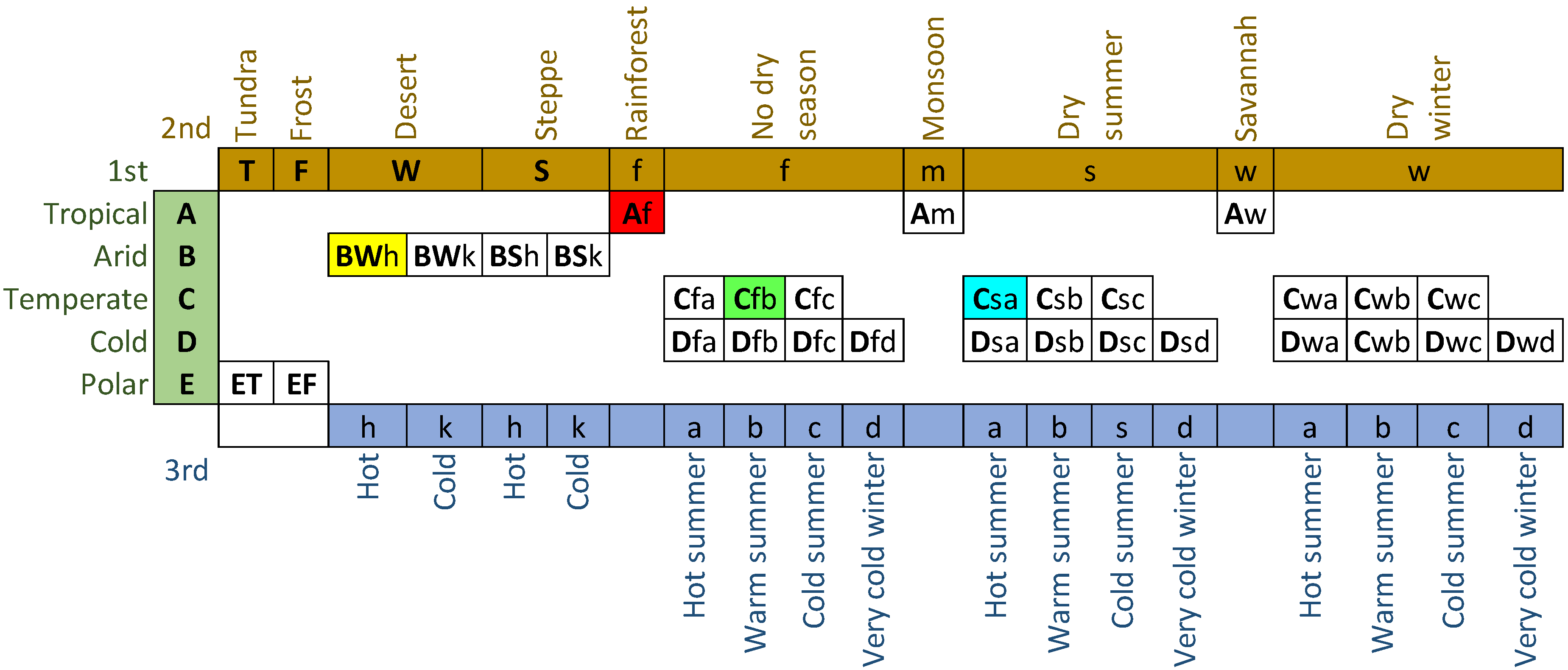
| Country, City | Climate Class | Description | |||||||
| Italy, Bolzano | Cfb | Temperate, no dry season, warm summer | p-Si (210W) | −0.457 | 4.20 | SMA SB 4000TL | 30 | 188.50 | 29.70 |
| Indonesia, Pekanbaru | Af | Tropical, rainforest | p-Si (PS 220-6P-S) | −0.490 | 1.76 | SMA SB1700 | 10 | 180.00 | 13.14 |
| Indonesia, Cirata | Af | Idem | p-Si (ASL-M100E) | −0.480 | 5.00 | SMA SMC 5000 | 10 | 15 | 33.50 |
| Australia, Alice Springs | BWh | Arid, desert, hot/Site 8 | p-Si (BP 3165) | −0.50 | 4.95 | SMA SMC 6000A | 20 | 0 | 37.75 |
| BWh | Idem/Site 11 | p-Si (BP 3165) | −0.50 | 4.95 | Idem | 20 | 0 | 37.75 | |
| BWh | Idem/Site 34 | p-Si (WSP-240P6) | −0.45 | 5.28 | Idem | 20 | 0 | 36.59 | |
| BWh | Idem/Site 8 | a-Si (G-EA060) | −0.230 | 6.00 | Idem | 20 | 0 | 95.04 | |
| BWh | Idem/Site 17 | HIT (HIP-210NKHE5) | −0.30 | 6.30 | SMA SMC 7000TL | 20 | 0 | 37.83 | |
| BWh | Idem/Site 27 | CIGS (SL1-85) | −0.38 | 5.61 | SMA SMC 6000A | 20 | 0 | 49.48 | |
| BWh | Idem/Site 7 | CdTe (FS-272) | −0.250 | 6.96 | Fronius Primo 6.0 | 20 | 0 | 69.12 | |
| BWh | Idem/Site 23 | CdTe (CX-50) | −0.250 | 5.40 | SMA SMC 6000A | 20 | 0 | 77.76 | |
| BWh | Idem/Site 28 | CdTe (FS-387) | −0.250 | 5.60 | Idem | 20 | 0 | 46.08 | |
| BWh | Idem/Site 10 | mono-Si (SPR-215-WHT-I) | −0.38 | 5.81 | Idem | 20 | 0 | 33.59 | |
| BWh | Idem/Site 12 | mono-Si (BP 4170N) | −0.50 | 5.10 | Idem | 20 | 0 | 37.81 | |
| BWh | Idem/Site 13 | mono-Si (TSM-175DC01) | −0.45 | 5.26 | Idem | 20 | 0 | 38.37 | |
| Climate | Country | PR | PRstc. | PRann. |
|---|---|---|---|---|
| BWh | Australia | 0.81 ± 0.03 | 0.92 ± 0.02 | 0.81 ± 0.02 |
| Af | Indonesia | 0.81 ± 0.03 | 0.90 ± 0.03 | 0.81 ± 0.03 |
| Cfb | Italy | 0.84 ± 0.04 | 0.89 ± 0.03 | 0.84 ± 0.03 |
© 2020 by the authors. Licensee MDPI, Basel, Switzerland. This article is an open access article distributed under the terms and conditions of the Creative Commons Attribution (CC BY) license (http://creativecommons.org/licenses/by/4.0/).
Share and Cite
Kunaifi, K.; Reinders, A.; Lindig, S.; Jaeger, M.; Moser, D. Operational Performance and Degradation of PV Systems Consisting of Six Technologies in Three Climates. Appl. Sci. 2020, 10, 5412. https://doi.org/10.3390/app10165412
Kunaifi K, Reinders A, Lindig S, Jaeger M, Moser D. Operational Performance and Degradation of PV Systems Consisting of Six Technologies in Three Climates. Applied Sciences. 2020; 10(16):5412. https://doi.org/10.3390/app10165412
Chicago/Turabian StyleKunaifi, Kunaifi, Angèle Reinders, Sascha Lindig, Magnus Jaeger, and David Moser. 2020. "Operational Performance and Degradation of PV Systems Consisting of Six Technologies in Three Climates" Applied Sciences 10, no. 16: 5412. https://doi.org/10.3390/app10165412
APA StyleKunaifi, K., Reinders, A., Lindig, S., Jaeger, M., & Moser, D. (2020). Operational Performance and Degradation of PV Systems Consisting of Six Technologies in Three Climates. Applied Sciences, 10(16), 5412. https://doi.org/10.3390/app10165412