Quantification of the Benefits for Power System of Resilience Boosting Measures

Featured Application

Integration of a proposed resilience modeling framework within an approach for the optimization of measures to boost power system resilience.

Abstract

Severe natural events leading to wide and intense impacts on power systems are becoming more and more frequent due to climate changes. Operators are urged to set up plans to assess the possible consequences of such events, in view of counteracting them. To this aim, the application of the resilience concept can be beneficial. The paper describes a methodology for power system resilience assessment and enhancement, aimed at quantifying both system resilience indicators evaluated for severe threats, and the benefits to resilience brought by operational and grid hardening measures. The capabilities of the methodology are demonstrated on real study cases.

1. Introduction

Extreme events are affecting power systems more and more frequently, with consequent infrastructure disruption and loss of load supply. Transmission System Operators (TSOs) are thus pushed to evaluate the impact of multiple, weather-dependent outages of components, potentially leading to widespread blackouts, with the final aim to set up preventive and/or corrective measures to absorb the effects of such disruptive events and to recover fast. This objective can be concisely stated as increasing system resilience [1,2], and it is consistent with the more stringent requirements posed by regulatory entities [3].

Different types of measures can be considered to boost system resilience, in different time frames from long term planning to operational planning and real time operation. Long term measures may require months to years to be implemented, and typically aim to make components more robust (hardening measures). Operational planning and real time measures include systems for enhancing situational awareness and actions that can be activated within short time frames, e.g., changing the operating conditions or alerting repair crews (active measures).

In recent literature, some tools have been proposed to evaluate the benefits deriving from the deployment of hardening measures: For example, in [1] the authors evaluate the benefits from hardening solutions to boost UK grid resilience to storms by computing long term indicators typically used for reliability. However, little attention is paid to the modeling of operational measures: For example, in [4] the authors present a tool aimed at proposing optimal generation redispatching and grid reconfiguration actions to avoid damages of overhead lines (OHLs) due to wet snow sleeves. Reference [5] describes a tool which forecasts the potential outages due to tree falls on a distribution network by elaborating big amounts of data from different informative sources (historical series of failures, weather monitoring systems, etc.).

Operational measures for resilience enhancement can greatly benefit from big data analytics: In fact, big data applications can provide reasonable probabilistic models of a weather hazard for both long- and medium/short term analyses, respectively, through historical data series and through forecasts/quasi-real time data acquisition [5], which can support operators both in long term planning and in operation. Big data techniques are gaining importance in particular in the context of weather event alarms [6,7]: In [8] the authors propose a data driven tool for disaster management to support operators’ decisions in emergency conditions. Reference [9] describes a risk warning system also exploiting big data. In [10] a fuzzy logic system for decision making is proposed to help utility operators optimize real time operation and maintenance programs, with the final aim of mitigating weather impacts on distribution networks. This support from data analytics is even more precious if one considers the different threats to which power systems have been increasingly exposed in the last decades due to climate changes. In particular, wet snow events are common in many countries, e.g., Italy, and studies have focused on them for a lot of years [11].

The analysis of the benefits to resilience coming from different measures require a general framework rooted in an agreed resilience definition. In particular the choice of the best combination of grid hardening and operational measures to enhance resilience requires methods and tools able to quantify resilience by suitable metrics, to model the effect of the different measures to face threats of various intensities, and to assess the resilience improvement associated to the deployment of the measures. A first step towards a techno-economic assessment of the best portfolio of hardening and operational measures consists in a methodology able to quantify the technical benefits of these measures in terms of reduction of load disruption risk.

Each reference quoted above tackles individual resilience boosting measures but it does not provide a wide-ranging modeling frame allowing to model all the measures together, with the final goal to integrate them into a unified approach and tool for resilience enhancement.

The major novelty of the present paper with respect to previous literature is the formulation of a general methodological framework, based on an internationally agreed definition of resilience, supporting the assessment and the identification of the best solution to enhance resilience, keeping into consideration the specific characteristics of threats, faults, vulnerabilities, impacts by using specific models for the different boosting measures.

The framework proposes an innovative concept of risk with a more general interpretation of “vulnerability” property and it classifies the resilience boosting measures according to the definition of resilience [12] recently introduced by CIGRE (the International Council on Large Electric Systems) and to a cutting-edge relationship model between reliability and resilience derived from the definition itself. The new framework allows not only to assess the benefits of several kinds of boosting measures but also to perform sensitivity analyses on the parameters which characterize both the measures and the threats: In particular, it assesses measure effectiveness in boosting resilience for different threat severities and for different design choices of the measures.

To demonstrate the advantages coming from the framework, the paper applies it to several cases covering different key actionable measures deployed over different time frames: In fact, the general methodology can be applied both in operational planning, by anticipating critical situations, and in long term planning, by calculating the return periods of component outages. Moreover, the capability of the innovative methodology to perform “what if” analyses is shown in the paper.

The paper is organized as follows: Section 2 presents the overall methodological framework for resilience assessment and enhancement. Section 3 classifies the measures and Section 4 describes the models developed for the different measures. Section 5 presents and discusses the results of the application of the resilience assessment methodology to two case studies referring to transmission and distribution systems. Section 6 concludes.

2. A Framework to Model Power System Resilience

This section describes the framework developed by RSE to evaluate and enhance power system resilience, consistent with the recent CIGRE definition of resilience [12] which is initially recalled. The framework is preceded by a proposal on the relationship between resilience and reliability.

2.1. Resilience Definition From CIGRE C4.47

CIGRE WG C4.47 associates the concept of resilience to the system’s ability to limit the extent, severity and duration of system degradation following an event. As the criterion of application for this property mainly regards extreme events, the CIGRE WG C4.47 defines Power System Resilience as “the ability to limit the extent, severity and duration of system degradation following an extreme event”.

Several key measures can be used to achieve system resilience over different time frames (from short term to long term). The second part of the definition is dedicated to these key measures:

“Power system resilience is achieved through a set of key actionable measures to be taken before, during and after extreme events, such as:

• anticipation,
• preparation,
• absorption,
• adaptation,
• rapid recovery, and
• sustainment of critical system operation

including application of lessons learnt”.

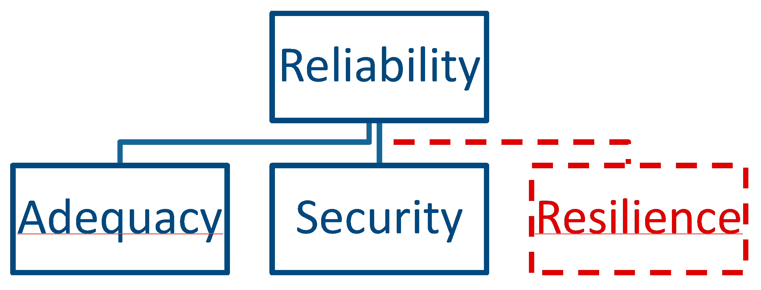
2.2. The “Three-Leg” Model to Link Reliability and Resilience

The Working Group C1 of CIGRE defined reliability as “A measure of the ability of a power system to deliver electricity to all points of consumption and receive electricity from all points of supply within accepted standards and in the amount desired” [13].

It is worth noticing that reliability definition does not refer to any specific application criterion (in particular, there is no reference to credible or extreme events).

Currently, security and adequacy are necessary conditions to verify the classical property of “reliability” for a power system. However, assuring the security of the system in case of multiple outages such as the ones produced by extreme events, would lead to unbearable costs in terms of component design, grid redundancy, system operation, and maintenance.

The resilience property addresses this aspect by imposing a less stringent requirement, i.e., to limit the degradation of the system. Accordingly, resilience can be added to reliability to characterize the system in the presence of any type of events. Under a broad perspective, reliability can be interpreted as a fundamental property which can be decomposed into three components: adequacy, security, and resilience (see Figure 1).

A reliable system must have enough available generation and transmission resources to feed the load with a suitable margin (adequacy), in case of the most limiting contingencies; it must withstand disturbances (security), i.e., continue to supply all the customers fulfilling suitable requirements, at least for the category of contingencies which satisfy a credibility criterion; but it must also limit its functional degradation (resilience) for those contingencies which do not satisfy the credibility criterion adopted by the TSO (extreme events).

This positioning of resilience as a sub-property of reliability is also justified by the following considerations. According to the classical reliability definition, a power system could not be defined reliable in case of extreme events. In fact, security, which requires no loss of load, is not assured for extreme events but only for credible contingencies. Instead, several advantages derive from stating that a necessary condition for a system to be reliable is that the system must have a sufficient resilience to extreme events:

• International definitions of reliability which do not include any references to the types of outages, are satisfied, including the recent definition proposed by CIGRE WG C1 [13].
• The definitions of security and adequacy remain unaltered.
• A clear link between resilience and well-known, widely adopted concepts is established.

This model is coherent with the definitions of FERC (Federal Energy Regulatory Commission of the US), NERC (North American Electric Reliability Corporation) and of the Italian national regulatory Authority, that considers both normal and exceptional (major force) events to evaluate the reliability. In particular FERC indicates that “resilience is a component of reliability in relation to an event” [14], and NERC states that “a bulk power system that provides an adequate level of reliability is a resilient one” [15]: This implies that resilience is a necessary condition for a reliable system.

In 2013 NERC introduced the definition of ALR “Adequate Level of Reliability” [16] of a Bulk Electric System (BES): ALR definition includes the typical requirements requested to a resilient system.

Reference [17] states “Within the broad context of reliability defined by these indices, resiliency would appear as a component of reliability. Resilience relates to restorability and speed of restoration”, highlighting that available reliability tools should consider the resilience of the system, by adequately modeling repair and restoration processes [18].

As indicated in [19] reliability is related to the ultimate goal of the power systems, i.e., providing electricity to the customers within specific standards for the service supply. Resilience is a good compromise for reliability attainment in case of extreme events, because it can specify the “standards for the service supply” in terms of maximum duration and severity of degraded performance of the system when it is struck by very severe events for which security cannot be assured at reasonable costs.

A system which is resilient is not necessarily reliable (because it may not comply with the service quality requirements, e.g., the maximum number and duration of supply interruptions, in case of credible contingencies). Moreover, a system which is reliable with respect to credible events (i.e., adequate and secure, according to the conventional definition of reliability) may not be resilient to events. However, a reliable system must have a sufficient level of resilience to extreme events, otherwise it would not satisfy the general definition of reliability under extreme events.

As a conclusion, according to the abovementioned broader interpretation of reliability, a reliable system must be adequate, secure for credible contingencies, and it must be enough resilient to extreme events. This statement holds valid for any credibility criterion adopted by TSOs.

2.3. A Risk Based Perspective to Analyse Power System Resilience

The assessment of power system resilience and its enhancement requires the re-definition of the boundaries of the system subject to the analysis. In fact, while the conventional concepts of security and adequacy are mainly focused on the power system only, resilience is a multifaceted subproperty which encompasses the relationship between power system and the (natural and human) environment. Resilience analysis hence focuses on the study of the interactions between the environment and the power system. The environment affects the system in different ways:

• Environmental threats can affect the infrastructure and energy supply service of power systems.
• Weather also influences the available generation and the load demand, thus the operating conditions of the power system (e.g., the large use of air conditioning systems in case of hot temperatures, the renewable generation as a function of wind speed and solar irradiation, and the cutoff of wind turbines due to excessive wind).

A resilience analysis always starts from the modeling of the root causes (e.g., wet snow storm) of the outages, namely natural or man-made threats. To this purpose, the bow tie model [20] provides a useful conceptual scheme to describe the connections between the different aspects of the resilience assessment framework. In particular, Figure 2 shows the bow-tie model used to qualitatively describe the connections between threats, component vulnerabilities, and power system contingencies.

The left side of the scheme in Figure 2 suggests possible classifications for threats, in particular two categories are highlighted: natural threats versus man-related threats, where the latter are in turn classified into internal or external to the power system. Threats act on power system components by means of stress variables (e.g., wet snow loads for a wet snow event) and they cause the faults of components by exploiting their vulnerabilities. Component faults lead to the occurrence of a contingency which may affect more or less components on the basis of the response of protection and automation systems. The contingency may lead to an initial impact which in turn can exploit other vulnerabilities, triggering a cascading process that finally results in load disruptions (up to widespread blackout). The barriers represented in Figure 2 stop (or at least make less probable) the overall process which leads from threats to load disruptions: For example, a barrier can either reduce the intensity of the threat or reduce the vulnerability of the component to the threat. Given a certain set of faulty components, barriers allow to reduce the extent and the severity of a contingency. The same contingency may in turn cause less impact if suitable barriers are deployed.

This process from threats to power system impacts is modelled in the proposed framework taking into account:

• The differences among the application contexts (long term planning, operational planning, real time control), which affect the types of measures that can be adopted in each time frame.
• The uncertainties affecting the assessment process, which depend on the chosen application context.

For example, in long term planning strong uncertainties affect both load and generation patterns as well as the extreme values of weather variables, while operational planning considers the short term forecasts of load and renewable generation, the conventional generation schedule, as well as the short term forecasts of the weather conditions in the subsequent 24–72 h. In real time control, the main uncertainties regard the response of protection, defense and automation systems during the shock absorption phase and on repair crew work in the recovery phase.

In this context, risk is a key enabler to take advantage of the concept of resilience. In particular, to catch the tight relationship between threats and contingencies, the classical concept of risk [21] as a triple (contingency, probability, impact) has been revisited and extended in the past: In [1,20] “probability” term has been replaced with “threat” and “vulnerability” terms. However, in the approach in [20], vulnerability is strictly connected to the ability of grid component to resist to the threat.

The adopted risk definition allows to link Probabilistic Hazard Assessment (PHA) to Security Assessment, moving the focus from the proximate to the root causes of disruption events.

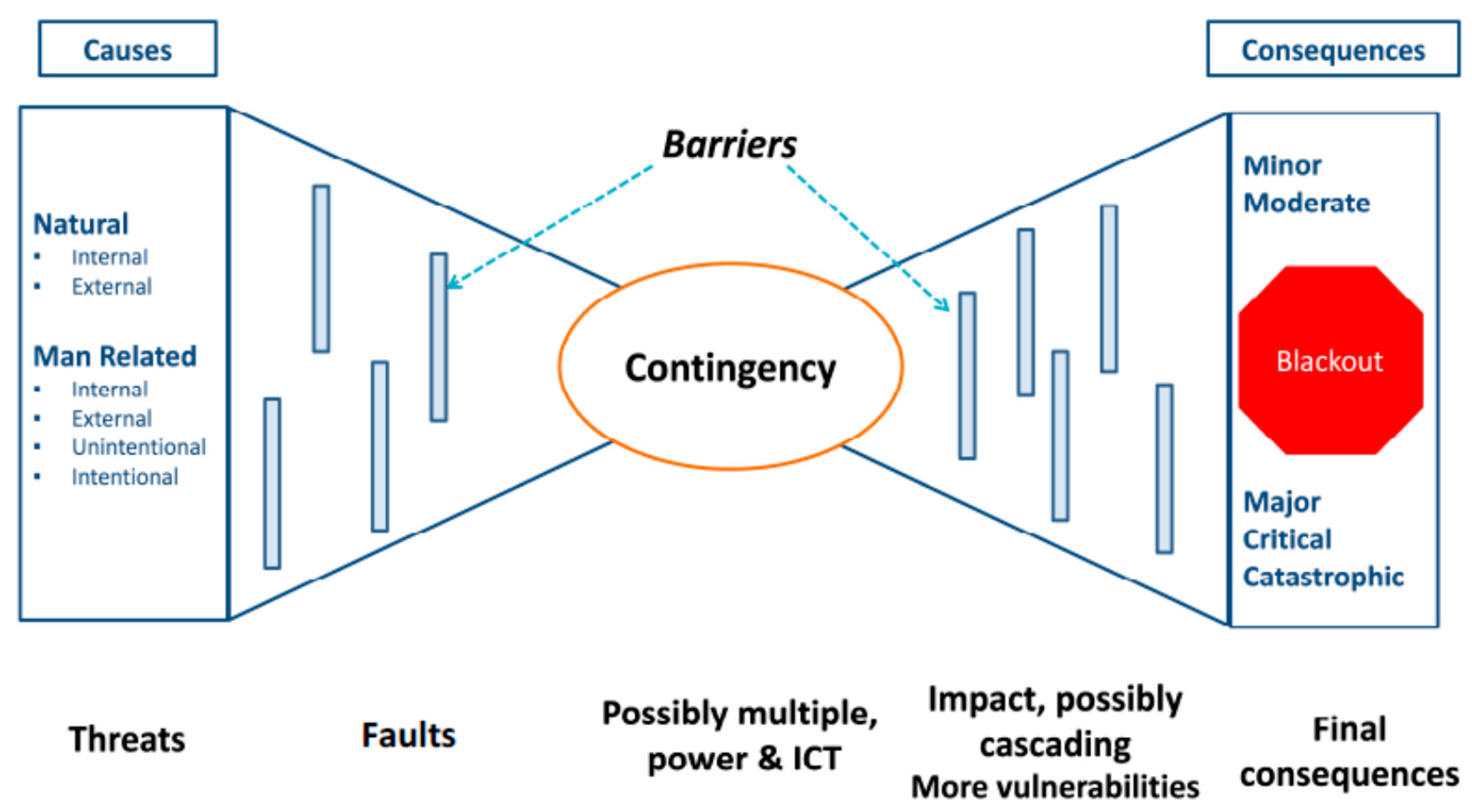
2.4. A Mathematical Formulation Derived from CIGRE Definition

Considering the CIGRE definition of power system resilience helps build a general mathematical formulation to fully quantify the system resilience by suitable metrics and the benefits to resilience obtained by deploying measures. The formulation in this paper proposes a generalization of the risk concept reported in [20] by interpreting the risk as a quadruple (threat, fault, contingency, impact).

Such a general mathematical framework includes the following variables:

• Threat, Th, characterized in probabilistic terms using a suitable probability distribution for the related stress variables as a function of time.
• The fault of the component, Fa, with a fault probability P_Fa(t) which is a function of time.
• The contingency, Co, meant as any combination of component faults with the response of the relative protection and automation schemes, with a probability of occurrence P_CO(t) which is again a function of time.
• The impact of contingency Co on the system, Imp, which can be expressed in terms of LOL (Loss of Load), ENS (Energy Not Served) and static and dynamic instability indicators, and described with a suitable probability distribution of the abovementioned continuous quantities, depending on the characteristics (load and generation patterns) of system state defined through appropriate stochastic variables S.
• Barriers B which can reduce the vulnerability of the grid components to the threat or the severity of a contingency. The barriers in Figure 2 are implemented by the key actionable measures in the CIGRE C4.47 resilience definition presented in Section 2.1.

Many factors of influence affect the intensity of threat Th, the probability of component faults Fa, the probability of occurrence and the impact Imp of contingency Co, as well as the power system state S. The most important factors consist in environmental factors W: e.g., the time evolution of weather variables and slowly varying or fixed characteristics of terrain (orography, tree coverage) determine the severity, the extent and duration of the threat stress on the grid infrastructure. Other significant factors may be organizational factors Z, such as the number of maintenance teams and the way to schedule their jobs, which affect, e.g., the duration of the recovery phase. This means in mathematical terms that Th, Fa, Imp, and Co are functions of W and Z, as well as of the deployed measures B. These measures can be classified into two categories, as described in detail in Section 3:

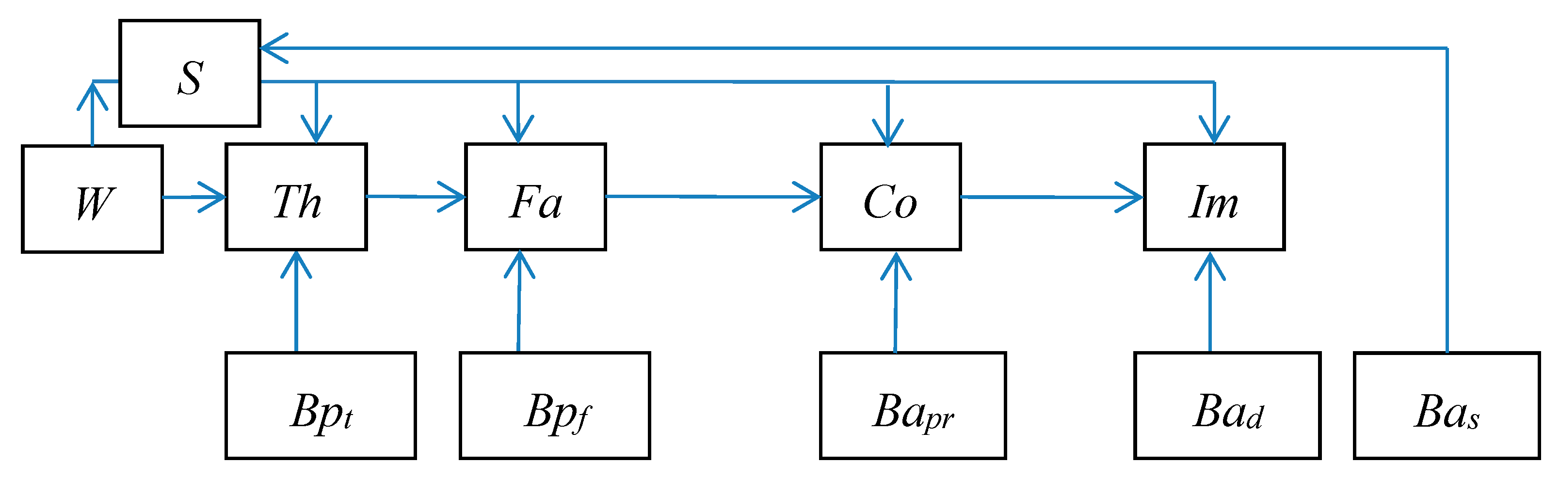
• Passive measures, defined with binary variables Bp.
• Active measures, defined with binary variables Ba.

In particular, passive measures mainly affect:

• The intensity of threat stress (indicated with Bp_t).
• The probability of having component faults (indicated with Bp_f), given a specific threat stress intensity.

Active measures typically affect:

• The extent, the probability of occurrence of a contingency (e.g., redundancy in protection systems, indicated with Ba_pr).
• The impact of a contingency, given a specific set of component faults (e.g., the defense systems, indicated with Ba_d).
• The state of the system S (e.g., the redispatching of conventional generators can bring the line current above anti-icing current which avoids wet snow sleeve formation). These measures are indicated by binary variables Ba_s.

System state S influences in turn all the other variables because it may affect:

• The threat intensity (e.g., if the line current is above a minimum anti-icing current, then the wet snow sleeve does not accrete on the conductor).
• The fault probability (e.g., a high current on a line causes an augmented sag and increases the probability of tree contact).
• The extent and the probability of occurrence of a contingency given a set of component faults (e.g., the probability of cut-out of wind farms depends on the system conditions).
• The impact of a contingency (e.g., cascading outages depend on post-contingency power flow).

Figure 3 reports the conceptual relationship among the variables.

Starting from the probability distributions associated to the weather variables, the methodology can derive the probability distributions of threat severity and combine them with the component vulnerability models in order to evaluate the probabilities associated to the faults of components (Fa) and to the occurrence of contingency Co.

Given a suitable metrics Imp to describe the extent, the duration and the severity of system degradation (e.g., the ENS or LOL) which depends on the specific contingency Co and on power system state S and on the measures deployed to counteract it, one can define the resilience metrics in two forms:

• Directly, as a function of a risk index given by a combination Θ of contingency probability P_CO and of its impact Imp (Co, S, Ba_d), with Co = Co (Fa (Th_Δ, S, Bp_d), S, Ba_pr) and Th_Δ = Th_Δ (W, Bp_t, S) by considering only the uncertainties related to the fault probability of components. $T{h}_{\mathit{\Delta }} is$ the probability distributions of the stress variables over the time interval of analysis $\mathit{\Delta }$.
• In probabilistic terms, as the probability that the risk metric above is lower than a specified threshold γ (established by TSO guidelines) over an interval of analysis $\mathit{\Delta }$ (ranging from few minutes for quasi real time control to years for long term planning), as follows:

  $$Resilienc{e}_{\mathit{\Delta }}=Prob\left(\mathsf{\Theta }\left(\begin{array}{c}{P}_{CO}\left(Co\left(Fa(T{h}_{\mathit{\Delta }}, S_{\mathit{\Delta }},B{p}_f\right), S_{\mathit{\Delta }}, B{a}_{pr}\right), \\ Imp\left(\left(Co\left(Fa(T{h}_{\mathit{\Delta }}, S_{\mathit{\Delta }}, B{p}_f\right), S_{\mathit{\Delta }}, B{a}_{pr}\right),S_{\mathit{\Delta }}, B{a}_d\right)\end{array}\right)<\gamma \right)$$

  (1)

  where $T{h}_{\mathit{\Delta }}$and $S_{\mathit{\Delta }}$ are the probability distributions of system state variables and of the stress variables over the time interval of analysis $\mathit{\Delta }$.

This form accounts also for the uncertainties on power system state.

These indexes can be calculated by accounting either for an individual contingency or for a set of contingencies.

Thanks to this new conceptualization of risk as a quadruple (threat, fault, contingency, impact), the property of vulnerability is much more general than in the previous definition of risk as the quadruple (threat, vulnerability, contingency, impact): In fact, in the latter one vulnerability only refers to the ability of components to resist to the threat, while in the new conceptualization of risk, the vulnerability is interpreted as the property which links any couple of quantities in the process of Figure 2, i.e., threat, fault, contingencies and impacts, following the cause–effect sequence (Th → Fa → Co → Imp).

Next sections will classify these measures and propose their mathematical models with some application examples to realistic grid models. The sequel of the paper will consider the former formulation of the resilience index. A brief description of the resilience index adopted in the simulations is given in the next subsection. The analytical development of Equation (1) is out of the scope of the present paper.

2.5. RELIEF: The Tool Implementing the Bow Tie Model

The bow tie conceptual model was translated into a methodology and implemented into a tool for power system resilience assessment named RELIEF [20,22,23,24]. Threats and component vulnerability models are combined thus leading to the failure probabilities of components, thus also the probability of occurrence of outages which can potentially provoke load disconnections [20].

RELIEF allows to assess power system resilience over different time frames. In the operational context, it combines the probabilistic models of the threats (e.g., lightning, fire, and wet snow) with the probabilistic models of component vulnerability in order to calculate the component failure probabilities, with a time horizon ranging from few hours to few minutes ahead. The step following the computation of the component failure probabilities consists in creating a quite exhaustive set of multiple, common mode and dependent contingencies affecting the components more prone to fail. After a fast screening of the generated contingencies, the retained ones are simulated via a quasi-static cascading outage simulator to assess possible cascading outages provoked by the initiating events. This allows to evaluate impact indicators such as the amount of MW not supplied or the energy not served. The risk based resilience indicator in case of generic contingency j in [20] is given by Equation (2).

$$Resilienc{e}_{ctg,j}=\frac{1}{Ris{k}_{ctg,j}}=\frac{1}{\left(p_{ctg,j}\times Im{p}_{ctg,j}\right)}$$

(2)

where $p_{ctg,j}$ is the probability of occurrence of the contingency, the impact indicator Imp_ctg,j is given by the loss of load (MW). The total risk of loss of load can be defined as the sum of the risk indicators Risk_ctg,j for all the most dangerous contingencies.

This means that the adopted risk metric$\mathsf{\Theta }$ in the general formulation is given by the product of contingency probability and impact.

The system resilience can be defined as the minimum of the resilience indicators among the set Ω of most dangerous contingencies to which the system is exposed, see Equation (3).

$$Resilienc{e}_{syst}=\underset{j\in \mathsf{\Omega }}{\min }Resilienc{e}_{ctg,j}$$

(3)

More comprehensive indicators include information about the restoration process, but the proposed indicator is currently adopted by the Italian National Regulator in cost-benefit analyses as reference indicator to be assessed by operators to justify the effectiveness of their investments. Thus, in the sequel this indicator will be calculated for all the measures under study.

RELIEF also includes a submodule which computes the time for infrastructure and electric service recovery depending on the weather forecasts: some applications of the submodule to a real emergency scenario due to wet snow in North of Italy are reported in [22].

The tool allows to characterize the threat geospatial models in the following ways:

(1)

In engineering mode, where a simple analytical model with few parameters is used to characterize the intensity and the extent of the threat as well as their uncertainties [20].

(2)

In operational planning mode, by integrating the k hour-ahead weather forecasts in order to build the probabilistic model of weather based threats.

(3)

In long term planning mode, by considering the weather-related geospatial distributions as the distributions of the annual extreme values of the stress variables (for each location). In this mode, the combination of extreme value distributions with the vulnerability models of grid components leads to the calculation of the return periods of component outages [24].

3. Classification of Resilience Boosting Measures

The key actionable measures mentioned in Section 2 and described in [12] characterize any power system: In fact, the adoption of defense plans to absorb the contingency impact, the upgrades of operating and maintenance procedures on the basis of past events, the scheduling of maintenance teams are only few examples of current practices of grid operators to face severe disruptive events. However, a resilient system should be capable to exploit these measures to achieve acceptable targets for the energy supply in case of extreme events.

The corresponding capabilities of the system to deploy the previous key measures, i.e., the anticipative, absorptive, adaptive, and restorative capabilities, must be quantitatively assessed by means of suitable metrics, so that it becomes possible to set objectives, to establish suitable strategies and measure the improvements, thus providing a valuable support to the decision making process.

A classification of the resilience boosting measures has been provided in [20] distinguishing:

• Passive approaches, with the goal of enhancing the capability of the infrastructure to resist in case of threats, by limiting their impact via redundancies, component hardening and protective mechanisms or barriers.

The first solution decreases the infrastructural vulnerability by introducing redundancies, e.g., by increasing the number of branches, thus improving the grid meshing. The other two measures decrease component vulnerability, avoiding that threats can damage the grid infrastructure: Some examples are the hardening of the lines, the maintenance of the rights of way (ROW) of the lines, the application of anti-torsional devices, the conversion of overhead lines into cables.

• Active approaches, with the goal of minimizing disruptions, enhancing system absorption capacity and speeding up the restoration process. Smart solutions for active approaches are:

  ○

  The assessment, forecasting and mitigation of threats.

  ○

  The scheduling of control actions which reduce component and system vulnerability.

  ○

  The defense plans, aimed to limit degradation process (hence, load disconnections).

  ○

  The restoration procedures, which must be adapted to the specific situation of disruption and the subsequent restoration process.

Passive approaches mainly refer to the design and the planning of components and of the grid; active ones refer to the design of smart protection and defense systems and of the actions which are to be taken during the operational planning and real time operation, which must be as “tuned” as much as possible on the actual situation in terms of threats and system condition.

In this context, methodologies based on the risk concept like the one presented in Section 2.3 assume a fundamental role: they allow to quantify the occurrence of extreme events and their impact on the system, and to identify effective planning and operation solutions also in case of significant threats. It should be noted that in many cases the adoption of passive approaches, such as expanding the grid with new power lines, can be subject to considerable delays due to the timing of authorization processes. From this point of view, whenever possible, the adoption of approaches or solutions based on the strengthening of existing infrastructures or plants may be preferable. Moreover, low-cost “operational” active measures for resilience enhancement deserve attention, especially if compared to large investments for grid hardening.

It is worth remarking the tight connection between CIGRE list of key actionable measures and the aforementioned classification of the resilience boosting measures. To this regard

Table 1. Examples of mitigation measures.

	Threats	Faults	Contingencies	Impacts
Anticipation	Weather prediction and event monitoring and alarm systems.	Predictive DLR (Dynamic Line Rating).	Multiple contingencies and their probability.	Loss of load. Branch overloading. Under/Overvoltages.
Preparation		Real time DLR Monitoring of transformers temperature Monitoring of leakage currents.	Wide area monitoring functions (WAMS) in SCADA.	WAMS for higher situational awareness.
Absorption	Dispatch of active and reactive powers for anti-icing and de-icing.	Controlling the clearance from ground by decreasing line currents, to avoid flashover. Increasing the line sag to increase the admissible snow sleeve load. Operating the grid components at lower voltages to avoid insulator flashover. Reduction of power imbalances among areas to decrease the vulnerability of grid corridors.	Substation reconfiguration aimed at reducing the probability of multiple contingencies. Fast reclosure. Slow reclosure. Adaptive protection systems for multiple contingencies with fast configuration changes.	Post contingency reconfigurations to decrease operational risk.Coordinated voltage and frequency control. Counterfeeding also between different voltage levels. Redispatching. Adaptive SPS (Special Protection Systems). Adaptive controlled islanding based on predictions and preventive redispatching. Response based and event based defense plans.
Sustainment of critical system operations	-	-	-	Deployment of additional components (for example, mobile generator), systems (e.g., uninterruptible power supplies).
Rapid recovery	-	-	-	Optimal scheduling of maintenance teams. Enhance communications and connections with Civil Protection and other public authorities.
Adaptation	Upgrades of prevention barriers and maintenance procedures.	Upgrades of prevention barriers and maintenance procedures.	Upgrades of operational procedures and regimes.	Upgrades of operational and maintenance procedures.

reports some examples of mitigation measures in relation with the key actionable measures indicated in the CIGRE definition and the bow tie model.

The same measures can be classified according to other criteria:

• The time horizon when the measures are applied.
• The activation depending on the actual occurrence of the disturbance.

The classification at point 1 leads to two categories:

• Measures planned over a multi-year horizon (planning).
• Measures adopted on a multi-hour horizon (operational planning).

The classification at point 2 leads to two categories:

• Measures activated before the occurrence of the disturbance (preventive).
• Measures activated after the occurrence of the disturbance (corrective).

The modeling of the measures implies a close collaboration between experts from different fields (structural, electrical, ICT engineers). Moreover, the modeling of many measures is strictly connected to the specific threat to be studied (e.g., the modeling of anti-torsional devices is useful to study the vulnerability of grid infrastructure to wet snow threat). Other measures are common to all threats: e.g., the defense systems act to limit the cascading outages originated from a contingency, no matter which threat originated it.

This introduction is important to understand the following sections, which will present the models of both general measures, and threat-specific measures: The latter are mainly focused on the wet snow threat.

4. Modeling Framework for the Measures

This section describes the modeling framework for measures which are either general or threat-specific. In order to focus the discussion, unless differently specified, the wet snow threat is considered in the following.

Wet snow events have often struck the Italian Extra-High Voltage (EHV) transmission system in the last decades [11,25], provoking significant damages to overhead lines due to the combined action of wind and wet snow loads.

4.1. A General Active Measure: Contingency Forecasting

One of the functions of RELIEF is contingency forecasting [23], i.e., the ability to anticipate the most risky contingencies which may affect the system in the subsequent hours, on the basis of the forecasted evolution of the weather threat and the vulnerability curves of the power system components.

As an example, in case of wet snow events, the stress variables (e.g., the mechanical tension on conductors and the load on cross-arms) present a geospatial distribution which depend on the spatial distribution of the related weather variables (e.g., wind speed and precipitation rate) on the basis of causal physical models (e.g., the Makkonen model [26] which links the weather conditions with the thickness of wet snow sleeve on a conductor): this model must also take into account the forecast uncertainties which characterize weather variables.

In particular, in the operational planning mode the tool considers the k hour-ahead forecasts provided by numerical weather prediction systems to get an affordable probabilistic model for weather-based threats.

Wet snow event modeling requires the forecasts of ambient temperature, precipitation rate, wind speed and direction, which come from numerical weather prediction models (NWP). Contingency forecasting is a general measure because it allows to anticipate critical conditions in case of threats other than wet snow, for example pollution [27] and tree fall [28].

4.2. Modeling of Threat-Specific Active Measures for Wet Snow Events

As for active measures, several methodologies and software tools have been developed by RSE, aiming to support power system operation in presence of extreme weather events. Among others, the following are briefly described below: A security-constrained generation redispatching for the transmission grid, an OPF-based identification of measure to assure minimum anti-icing current on medium voltage (MV) networks and an optimal reconfiguration of counterfeeds of the distribution grid to speed up the recovery process.

4.2.1. Security-Constrained Generation Redispatching

An active measure modelled within the RELIEF tool in engineering and operational planning modes consists in the redispatching of generation aimed to assure a minimum anti-icing current on the branches most subject to wet snow sleeve accretion, both in transmission system and in distribution networks [29,30], where it is possible and effective.

In particular the following functions are implemented:

• A security constrained redispatching (SC-R) [29] of the active powers injected by conventional dispatchable generators in the EHV/HV transmission system: the redispatching costs of generators are minimized while assuring (1) the fulfillment of N and N-1 security constraints, and (2) a minimum current on the HV branches which present a high probability of failure in the pre-redispatch condition, due to the potential formation of wet snow sleeves. This SC-R accounts for the process of wet snow sleeve formation during the whole forecasted duration of the event, considering the changes in load/generation patterns and the minimum current values which are updated via advanced NWP models [11]. The minimum current is set with the aim to prevent ice formation thanks to the heat dissipated by Joule effect in the conductor.
• An OPF-based measure [30] which sets the generators’ active and reactive power setpoints with minimum and maximum current constraints on the branches of the MV feeders, considering the availability of some active measures (re-dispatching of generation and voltage regulation by acting on the tap position of On-Load Tap Changers, OLTC, at HV/MV substation transformers).

More details about the mathematical formulations of these measures can be found in [29,30].

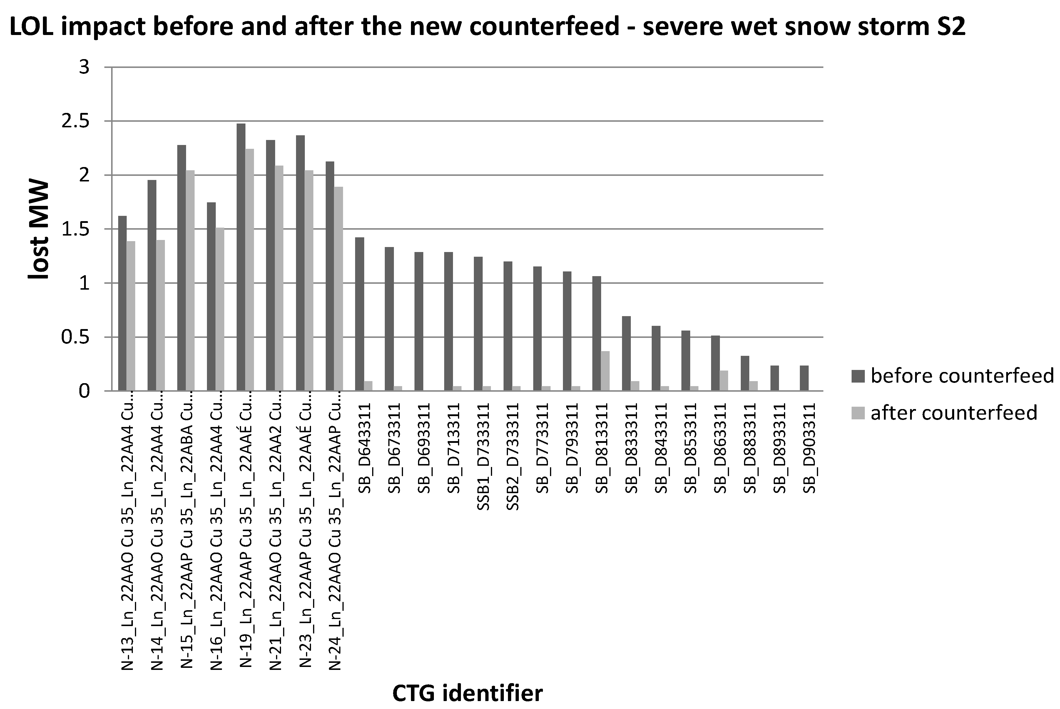
4.2.2. Optimal Reconfiguration of Counterfeeds to Speed Up the Recovery Process

The process of reconfiguring the counterfeeds following a contingency that determines the out of service of components of the network (for example MV connections, or secondary or primary substations) can have several objectives:

• Maximization of the load restored to users (primary objective).
• Minimization of the number of maneuvers (secondary objective).
• Reduction of active losses in the post-contingency network configuration.

The methodology adopted for the assessment of the impact of the contingency on the electricity supply service to users exploits the modified Viterbi algorithm [31].

The problem is formulated as follows: find the status (closed or open) of all the counterfeeds to maximize the amount of restored loads of the disconnected users (target objective) with the minimum number of maneuvers on the counterfeeds (secondary objective) and ensuring the fulfillment of the following constraints:

• Static security (no violations of the voltage magnitude and phase angle at the nodes and no overloads on the branches).
• Radiality condition of the connected network.

In case that multiple solutions are found that meet these constraints and the optimum criterion, then some performance metrics are considered to find out the “best solution” by filtering the less performing ones. These metrics are:

• The minimum value between the voltages at the network nodes.
• Active power losses.

4.3. Modeling of Threat-Specific Passive Measures

Different passive measures to boost system resilience are being studied to reduce the wet snow sleeve [25]. As an example, mechanical stabilizers of the conductors aim at avoiding or limiting the conductor rotation which provokes sleeve growth. Ice-phobic coatings can delay the sleeve formation by decreasing wet snow sticking capability on the conductor or favor sleeve shedding.

This subsection presents the models of some passive measures applied to transmission grid and focusing on wet snow threat: Anti-torsional devices, hydrophobic coating, upgrading of overhead power lines, conversion from airline to cable line, and building of new overhead lines.

4.3.1. Anti-Torsional Devices

These devices raise the torsional stiffness of conductors and they are deployed to prevent the beginning of the process which causes the wet snow sleeve to accrete [25]. The effect of anti-torsional devices has been studied in literature for a long time [32], even if further experimentation is needed to fully demonstrate the effectiveness of these devices. The device causes an increase of torsional rigidity, which limits or prevents the conductor rotation, thus the wet snow sleeve accretion. First of all, the model has to realistically quantify the rotation reduction due to these devices. Reference [32] can help in this task, by proposing some quantitative considerations about the observed decrease of ice loading after applying one or four anti torsional devices. Reference [33] proposes an analytical model which quantifies the reduction of ice loading on conductors in line with the findings of the experiments above.

In particular, the function F(x, N) in Equation (4) represents the rotation at distance x from one line terminal in case of N anti-torsional devices: the curve derives from the superposition of the absolute value of sin function along the line span with a maximum rotation of 19° (adequate value at design stage) on the absolute value of a shorter period sin function.

$$F\left(x,N\right)=max\left(0,\left(a-b{N}^c\right)\times \left|sin\left(\frac{\pi ·x·\left(1+N\right)}{L}\right)\right|+d\times \left|sin\left(\frac{\pi ·x}{L}\right)\right|\right)$$

(4)

In Equation (4) L is the span length, while the values for parameters a, b and c are derived by trial and error technique from [32]: a = 71, b = 12, c = 0.7, d = 19. The reduction factor (RF) is defined as in Equation (5).

$$RF=\frac{mean\left(min\left(F\left(x,N\right),F\left(x,0\right)\right)\right)}{mean\left(F\left(x,0\right)\right)}$$

(5)

RF is multiplied by the wet snow accretion intensity I₀ in the Makkonen model [26] to derive the derated intensity. The basic assumption is that the accretion intensity reduction is proportional to the reduction of the rotation angle.

4.3.2. Superhydrophobic Coatings

Hydrophobic or superhydrophobic materials can be used to build the anti-icing coatings. Although research is still ongoing, it is possible to model the coating action as a delay in the formation (sticking) of the first snow layer on conductor surface. Moreover, the ambient temperature is of paramount importance to quantify ice and snow adhesion forces to a metallic substrate [34,35]. The study of complex temperature dependent phenomena at conductor/snow interface [36] suggests adopting a time variant collision factor α₁(t), which depends on ambient temperature T_amb(t), as in Equation (6), in the Makkonen model [26].

$${\alpha }_1\left(t\right)=\{\begin{array}{c}0 if T_{amb}\left(t\right)<-0.5°C AND t-t_0\le TLIM\\ 1 otherwise \end{array}$$

(6)

In Equation (6), TLIM is the delay assured by the coatings (in hours) and it depends on the specific action mechanism of the coating and on environmental conditions where it operates, while t₀ is the starting time of the wet snow accretion phenomenon.

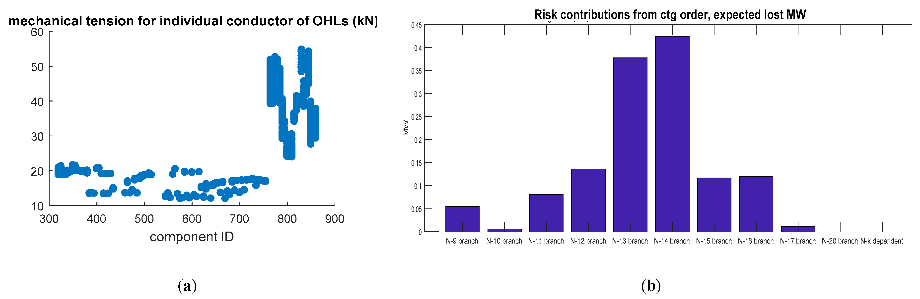
4.3.3. Upgrading of Overhead Power Lines

The upgrading is often chosen after recognizing the end of the operational life of the plants or the inadequacy of the current characteristics in case of the new climate conditions. The line is rebuilt preserving the existing layout and the general characteristics, but trying to improve the mechanical performance.

To this purpose, the process calls for the use of structures and components whose mechanical strength is increased and/or calculated with respect to recent regulations which require greater performance. In some cases, the resilience increase is obtained with a non-usual structure of conductors in order to reduce the frequency of faults due to wet snow overloads.

In some cases, the reconstruction may include the modification of the line layout in order to avoid the areas which are more prone to combined ice and snow loads.

4.3.4. Conversion from Overhead Line to Cable Line

The choice of burying an overhead power line must be strongly motivated by the greater reliability of the cable lines, not otherwise obtainable with aerial solutions, or by the need to improve the quality of the territory and meet other objectives agreed with the local communities. Evidently, the cable lines are immune from “ice or snow” events, but they are vulnerable to lightning and determine some problems to protection systems in case of alternating aerial and underground sections. Moreover, heat waves may damage cable junctions, also on the basis of the thermal properties of the soil. Thus, the generally partial conversion of overhead lines into cables must follow a cost/benefit analysis and an assessment of the consequences on the grid operation.

4.3.5. Building of New Overhead Lines

Network development has the goal of improving system reliability. The case of a HV/MV substation powered by a single line deriving from other plants, like other HV/MV substations or lines with 3 or more terminals is a typical situation where network development may play an important role. The goal is to assure a topology where each HV/MV substation is connected to two lines in “in-out” configuration. This produces meshes that satisfy the sufficient condition to obtain the current standards required for the quality of the electrical service. However, the new overhead lines have the highest cost among the interventions to increase the resilience, therefore they must be carefully justified.

5. Case Studies

This section summarizes some applications of the framework to model measures in both transmission and distribution systems.

5.1. Grids Under Study and Simulation Cases

The power grids where the methodology has been applied are:

• GRID 1: A model of the Italian High Voltage (HV, 132/150 kV) and Extra-High Voltage (EHV, 230/400 kV) grid which includes 5500 electric nodes, 8000 lines, 800 generators [20].
• GRID 2: a combined T&D system consisting in two MV feeders connected to a portion of the surrounding HV/EHV transmission grid in Aosta Valley, specifically around HV/MV primary substation at Villeneuve, particularly critical in terms of operation and maintenance as it provides energy to a very large area (about 770 km²) [37,38]. The model includes 92 MV electrical nodes, of which 60 nodes are MV/LV substations, 29 transit nodes in correspondence of line poles, and 3 MV nodes at Villeneuve HV/MV substation. The model includes three counterfeeds, 10 HV (132 kV) nodes, 8 EHV (220 kV) nodes, 20 OHLs, 6 generators and 3 EHV/HV transformers.

The goals of the simulations are:

(a)

To validate the methodology in operational planning mode (OP) by proving its effectiveness in anticipating the set of most risky contingencies.

(b)

To carry out a sensitivity analysis in engineering mode (EM) accounting for various threat intensities and measures, with the goal of quantifying the benefits to resilience.

(c)

To calculate the return times of component outages in long term planning mode (PL), for specific characteristics of component vulnerability.

The model to forecast the combined ice and wind loads accounts for four main exogenous variables i.e., the wind speed intensity and direction, the ambient temperature and the precipitation rate. The probabilistic vulnerability model of the OHLs in case of wet snow includes the vulnerability of phase conductors, shielding wires and tower equipment (e.g., bracings).

The simulation scenarios focus on two threats: Wet snow events, and tree falls due to combined wind and snow loads.

As far as wet snow events are concerned, the simulated scenarios are aimed to quantify the benefits of the following measures:

• Active measures: Forecasting of contingencies under critical conditions, Generation redispatching in transmission system to assure minimum anti-icing current requirements; OPF based measure acting on generators setpoints and OLTC in distribution networks to assure minimum anti-icing current requirements; optimal reconfiguration of counterfeeds to restore full load at the best post-contingency operational conditions.
• Passive measures: Anti-torsional devices; super-hydrophobic coatings, branch reconductoring, construction of new branches.

All of the use modes of the resilience assessment tool are adopted in the case study. In particular:

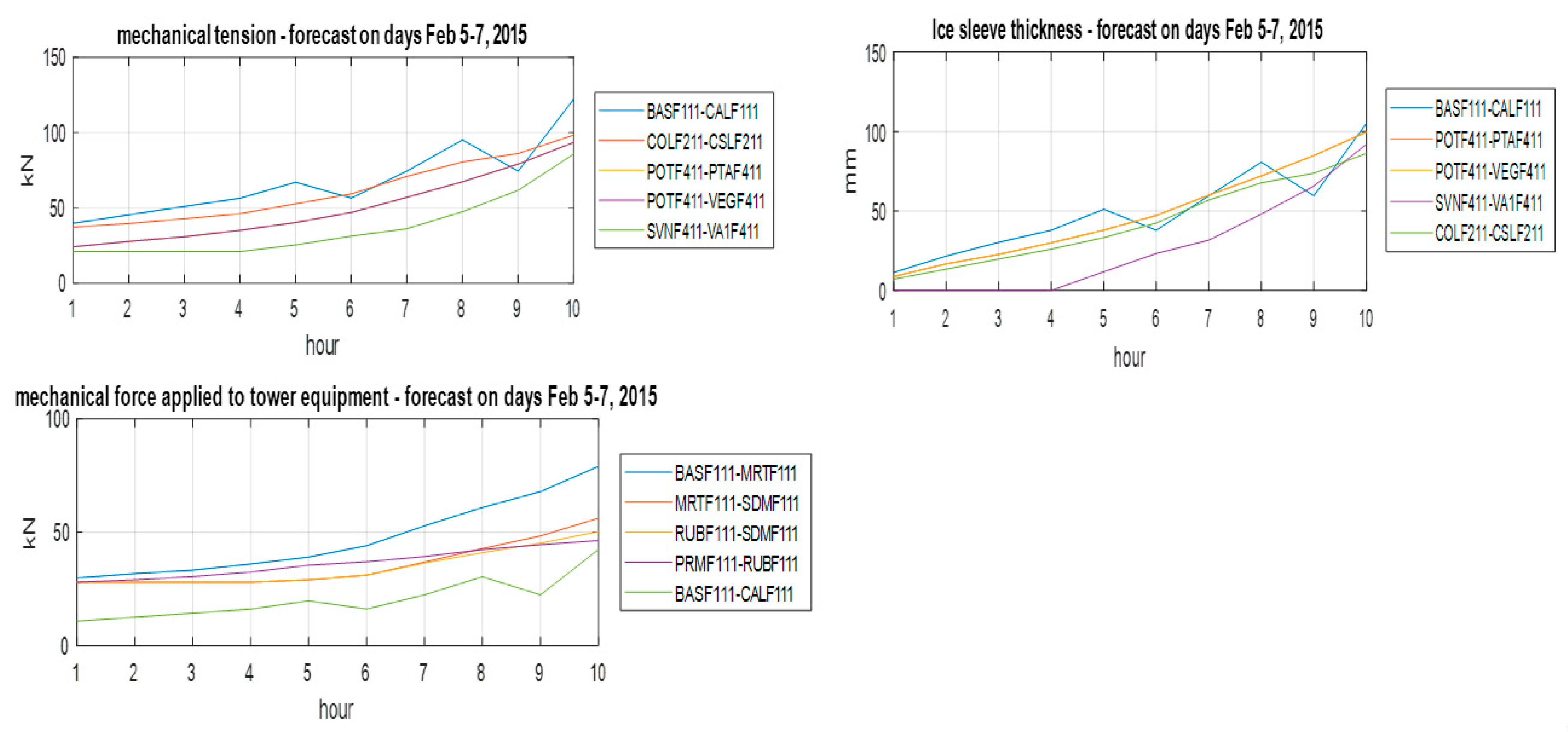
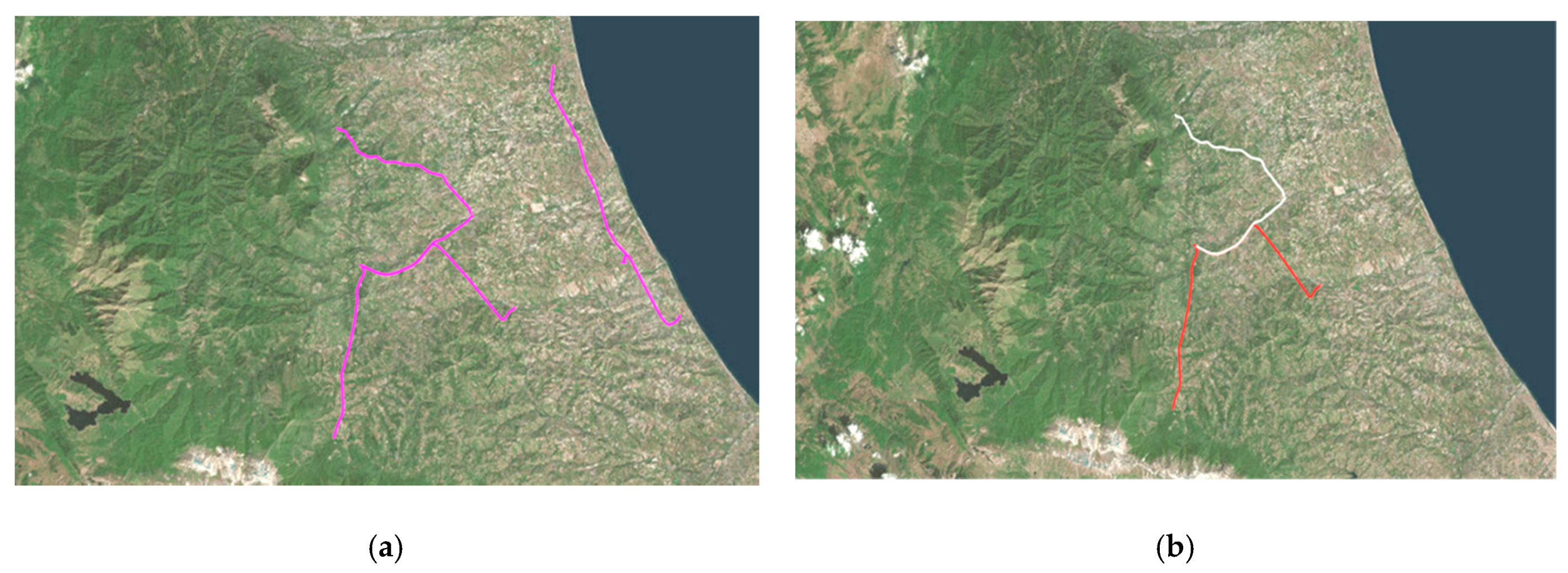
• A real wet snow event affecting the North of Italy in February 2015 is analyzed in the operational planning mode. To this purpose, the tool is fed by the 72 h ahead forecast of weather variables, thus forecasting the riskiest contingencies affecting the area.
• Wet snow events with different intensities are applied to the Central part of Italy in the engineering mode, considering different active and passive measures, characterized by different parameters.
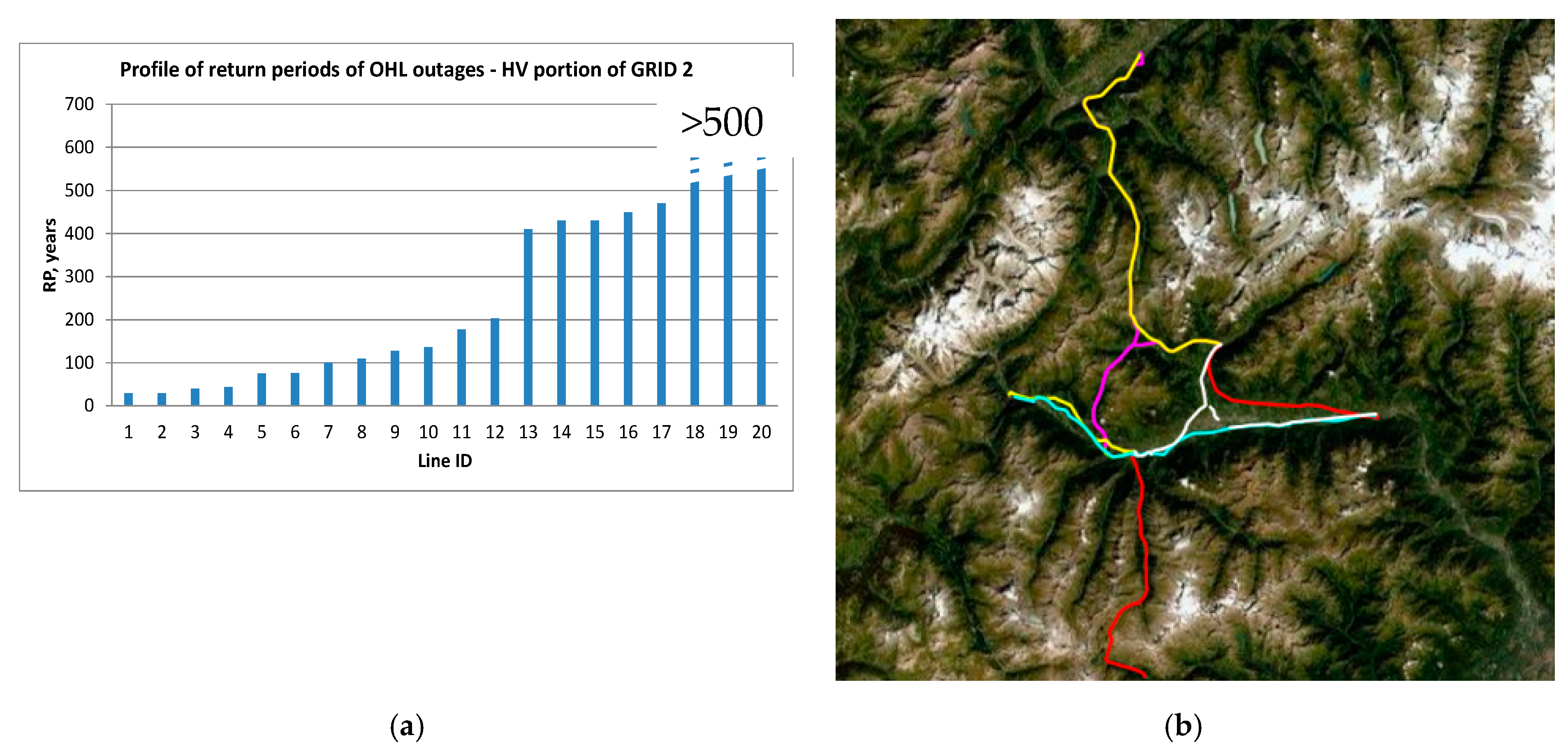
• The extreme value distributions provided by Std EN 50341-2-13 [39] for area 1 (North of Italy) are used in long term planning mode, with the aim of calculating the return periods (RPs) of OHL outages due to combined wind and wet snow loads in the portion of HV and EHV transmission grid in the GRID 2 model.

Table 2. Summary of the simulation cases.

Case	Grid Under Test	Affected Area	Mode	Threat	Measures
PL1	Base case GRID 2	HV portion	PL	Wet snow	Computation of return periods of outages
PL2	Base case GRID 1	HV grid of Sardinia	PL	Pollution	Comparison of return periods of outages with different insulator vulnerabilities
OP1	Base case GRID 1 adapted to Feb 2015 conditions	North of Italy	OP	Wet snow	Contingency forecasting
EM2	Base case GRID 1 + moderate wet snow event S2	Central Italy	EM	Wet snow	Resilience analysis
EM2-T	Base case GRID 1 + moderate wet snow storm	Central Italy	EM	Wet snow	Anti-torsional devices with interdistances 50 m/100 m
EM2-C	Base case GRID 1 + moderate wet snow storm S2	Central Italy	EM	Wet snow	Hydrophobic coatings with different delays 3/6/9 h
EM2-A	Base case GRID 1 + moderate wet snow storm S2	Central Italy	EM	Wet snow	Generation redispatching
EM1	Base case GRID 1 + severe wet snow storm S1	Central Italy	EM	Wet snow	Resilience indicators for sensitivity analyses
EM1-T	Base case GRID 1 + severe wet snow storm S1	Central Italy	EM	Wet snow	Anti-torsional devices with interdistance 50/100 m
EM1-C	Base case GRID 1 + severe wet snow storm S1	Central Italy	EM	Wet snow	Hydrophobic coatings with different delays 6/9/3 h
EM1-A	Base case GRID 1 + severe wet snow storm S1	Central Italy	EM	Wet snow	Redispatching of conventional generators
EM3	Base case GRID 2 + severe wet snow storm S1	T&D system	EM	Wet snow	Resilience indicators for sensitivity analyses
EM4	Base case GRID 2, moderate wet snow storm S2	T&D system	EM	Wet snow	Resilience indicators for sensitivity analyses
EM3-A1	Base case GRID 2 + severe wet snow storm S1	T&D system	EM	Wet snow	Optimal reconfiguration for counterfeeds
EM4-A2	Base case GRID 2 moderate wet snow storm S1 currents	T&D system	EM	Wet snow	OPF based active measure
EM3-P1	Base case GRID 2 + severe wet snow storm S1	T&D system	EM	Wet snow	Construction of a new counterfeed
EM4-P2	Base case GRID 2 + moderate wet snow storm S1	T&D system	EM	Wet snow	Reconductoring of small section branches
EM5	Base case GRID 2	T&D system	EM	Tree fall	Resilience indicators for sensitivity analyses
EM5-P1	Base case GRID 2	T&D system	EM	Tree fall	Enlargement of ROW
EM5-P2	Base case GRID 2	T&D system	EM	Tree fall	Trimming of tree height

summarizes the simulation cases described in the study.

In order to demonstrate the flexibility of the methodology to deal with different threats, some simulation cases in Table 2 refer to threats different from wet snow events, i.e., simulation cases EM5- * referring to tree fall due to wind and ice loadings, and case PL2 referring to pollution on component insulators.

The features of the moderate and severe storms run in the engineering mode are in

Table 3. Expected values for parameters characterizing wet snow event scenarios.

Hazard Parameter	Measurement Unit	Severe Storm (S1)	Moderate Storm (S2)
Peak wind speeds	m/s	10–15	10–5
Precipitation rate	mm/h	2	1
Initial precipitation level	mm	20	30
Air temperature range	°C	−0.6 (for S1m scenarios) 1 °C (for S1p scenarios)	−0.6

.

5.2. Calculating the Return Periods of OHL Outages due to Wind and Wet Snow Loads (PL1)

This long term planning application of the methodology consists in evaluating the RP of outages of the OHLs due to combined wind and wet snow actions. The example refers to the HV and EHV lines of GRID 2 model. The extreme values of wet snow loads and wind loads are derived from Std En. 50341-2-13 for area 1 (that is the North of Italy) [39].

From Figure 4a it can be noticed that the minimum RP is 29 years. For all the lines, the weakest sub-component (i.e., the one with lowest RP) is the support composed by the cross-arms and the body. Figure 4b shows the OHLs of the region with different colors representing decreasing values of return period of outage (from longer RPs in white to shorter RPs in magenta).

In particular, the colormap in the following figure indicates: RP in the interval [0, 30] years with magenta color, RP in the interval (30, 50] years with red color, RP in the interval (50, 100] years with yellow color, RP in the interval (100, 300] years with cyan color, RP in the interval (300, Inf) years with white color.

The knowledge of the RPs of component outages is a fundamental element to compute the long term resilience indicators such as EENS (Expected Energy Not Served).

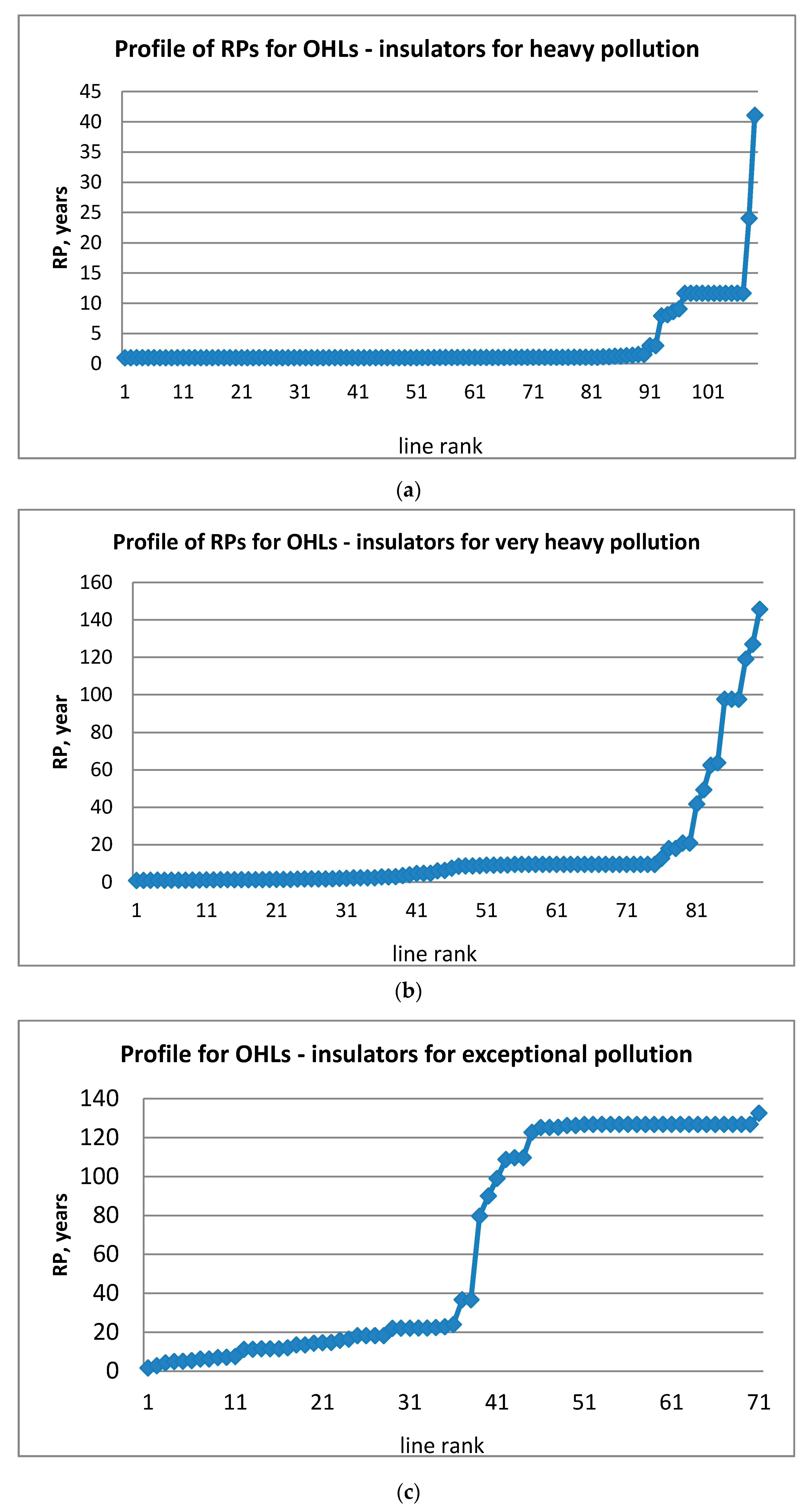
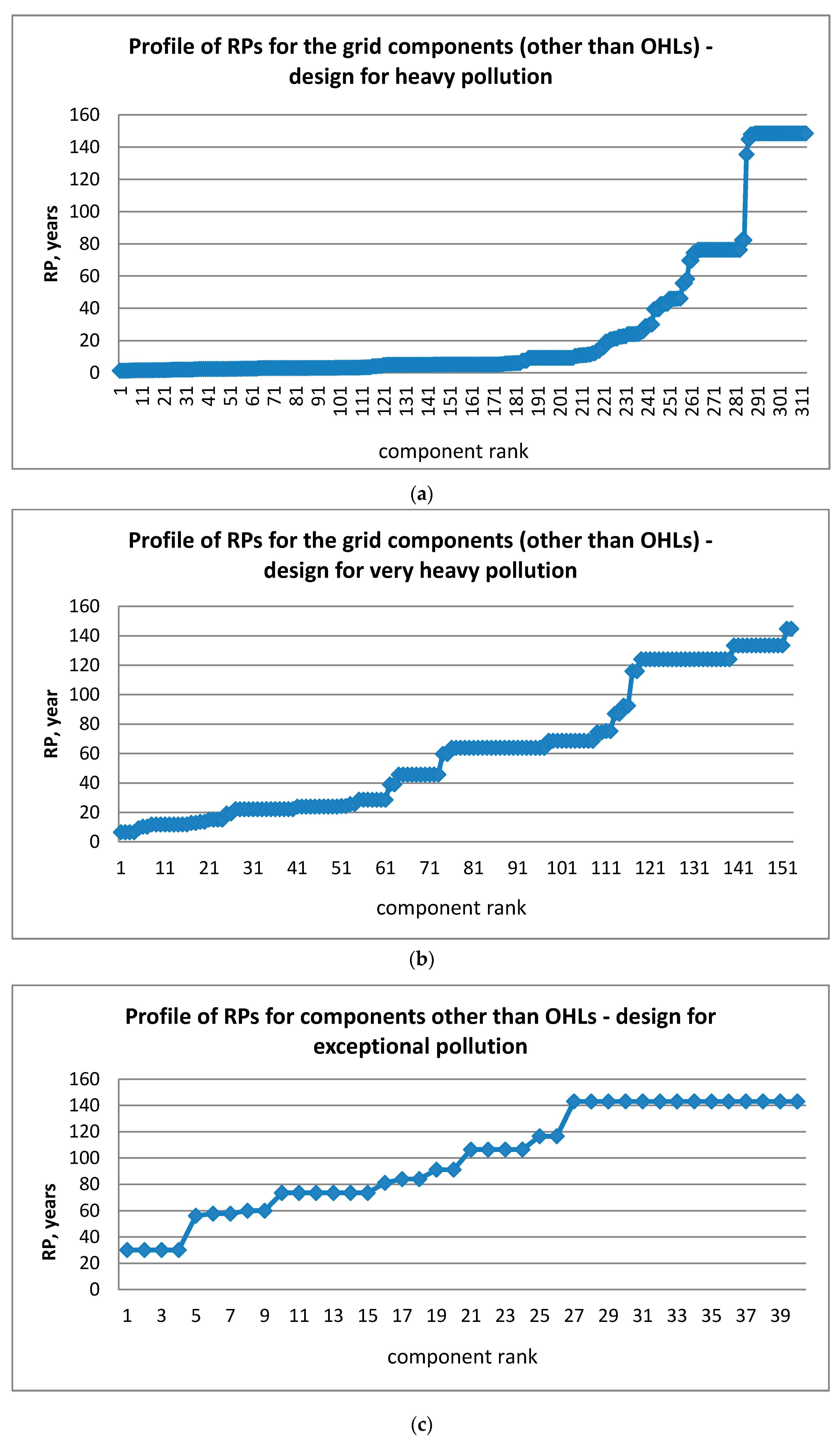
5.3. Comparing the Return Periods of Component Outages due to Pollution for Different Vulnerabilities of Insulators (PL2)

This subsection presents an application of the methodology in long term planning in order to assess the return periods of outages of grid components due to pollution for different vulnerabilities of component insulators.

In particular, the most important stress variable for “pollution” threat is the Salt Deposit Density (SDD) in mg/cm² even though also NSDD affects the vulnerability of the insulators to flashover. Thus, in the tests to demonstrate the effectiveness in applying the general methodology, only the map of SDD will be taken into account. The most vulnerable components are the insulator chains which are prone to flashover under polluted environments. In the present paper the authors adopt a voltage withstanding capability model for each insulator chain given by a three parameter Weibull distribution truncated for SDDs lower than a minimum value γ₀, as suggested in [40]. This distribution is characterized by the 50% flashover SDD γ₅₀ and parameters n, c and α.

The available maps provide the georeferenced distribution of the maximum values (over a two-year measurement campaign) of the SDD (Salt Deposit Density), in mg/cm², on the same type of insulators in the whole Italian peninsula in UTM coordinates. The measurements have been conducted on anti-salt glass insulators. The TSO guidelines indicate that in case of area with very heavy pollution (like Sardinia) then the minimum specific creepage length expressed in mm per kVrms maximum voltage at the terminals of the insulator chain should be included between 53 and 61 mm/kV: higher values of SCL are not advisable [30] and other measures should be deployed (such as special types/coverings for insulators, frequent cleaning of insulators).

$$A\times {\gamma }^{\alpha }=SCL$$

(7)

Equation (7) describes the relationship between SDD and the flashover voltage U [40].

Parameters A and α are derived from lab tests and depend on the specific type of insulator. Examples of values for parameters A and α can be found in [40] for some typologies of insulators.

Considering a value of SCL for 50% flashover equal to 54 mm/kV, and A = 54.4 and α = 0.22 as reported in [40], then the value of SDD which corresponds to the 50% probability of flashover reported in Equation (8).

$${\gamma }_{50}={\left(\raisebox{1ex}{$SCL$}\!\left/ \!\raisebox{-1ex}{$A$}\right.\right)}^{\left(\raisebox{1ex}{$1$}\!\left/ \!\raisebox{-1ex}{$\alpha $}\right.\right)}={\left(54/54.4\right)}^{\left(\raisebox{1ex}{$1$}\!\left/ \!\raisebox{-1ex}{$0.22$}\right.\right)}=1.05 \mathrm{mg}/{\mathrm{cm}}^2$$

(8)

Assuming a maximum value for SCL equal to 61 mm/kV leads to a γ₅₀ =(SCL/A)^(1/α) = (61/54.4) ^(1/0.22) = 1.68 mg/cm². In a similar way, for heavy pollution the estimated SDD value for 50% probability of flashover is 0.381 mg/cm².

In particular, a sensitivity analysis is performed on the 50% flashover SDD by considering the values 0.381, 1.05 and 1.68 mg/cm² for all the insulators of the island.

The other parameters n and c of the Weibull distribution remain the same and equal to the following value derived from [40]: n = 2.6 and c = 0.084.

The minimum value γ₀ of SDD which do not cause flashover depends on n, c, γ₅₀ and α: with the parameters analyzed for the present study the ratio γ₀/γ₅₀ is equal to 0.349.

It is worth noticing that all the mentioned parameters depend on the type and configuration of the insulator. In real world practice, specific solutions are studied for the grid portion and reasonable return periods are assured also using specific countermeasures such as silicone coverings. This study only intends to demonstrate the benefit to resilience which can be achieved by replacing the insulators with specific performances with higher performance insulators.

Specifically, simulation case PL2 compares the response to the same extreme values of pollution for insulators with three different design choices: heavy, very heavy and exceptional.

Figure 5 compares the profile of return periods for OHLs (considering RPs lower than 150 years) for the three sub-cases considered. Figure 6 compares the profile of return periods for other grid components (considering RPs lower than 150 years) for the three sub-cases considered.

In case of insulators designed for heavy pollution, it can be noticed that the RPs for lines and other components are generally higher than in the previous case, even though the RP values can still be too low in specific regions. In particular 207 components (other than OHLs) out of 1159 still show a RP lower than 10 years, only 57 components show a RP between 50 and 150 years. An area where still low RPs for OHLs and other components are detected corresponds to two portions of the Sardinian grid where pollution induced disturbances have recently taken place (extreme events of September 2001and October 2014).

In case of insulators designed for very heavy pollution, it can be noticed that fewer components (5 components) show a RP lower than 10 years: the areas with relatively low RPs are the North Western area and still the Southern area which underwent a series of pollution induced line trippings during the 2001 blackout of Sardinia.

In case of insulators designed for exceptional pollution, it is worth noting that all components have a RP higher than 30 years (the lowest RP is equal to 30.1 years) and that only ten lines at 132 kV have a RP lower than 10 years (with a minimum RP higher than 2 years). The area where the OHLs present the lowest RPs is still the Southern area mentioned for the previous subcases. The components with RPs lower than 50 years are identified in the South East part of Sardinian system.

This means also that a very conservative design of insulators considering the maximum advisable SCL for very heavy pollution conditions allows to limit and not to eliminate completely flashover problems: In real operation, additional measures (special silicone coverings, frequent cleaning of insulators, etc.) are to be deployed to further reduce the probability of occurrence of such severe events.

These simulations reach the goal to demonstrate that the proposed methodology can also assess the benefits (i.e., the increment of RP of component outage) achieved by adopting an increasingly performing design for the insulators, in a long-term planning horizon of analysis.

5.4. Contingency Forecasting in Operational Planning Mode (OP1)

This case study is an example of contingency forecasting application to a real emergency wet snow scenario occurred in The North of Italy on 5–7 February 2015. The forecasts of the weather variables of interest (ambient temperature, wind speed intensity and direction, precipitation rate) are elaborated on 4 February 2015 for the subsequent 72 h, and for each of the 11381 points of the forecasting geospatial mesh.

By applying the forecasts of weather variables to the grid model, it is possible to get the geospatial distributions of the stress variables of interest (wind and snow loads) for each hour belonging to the 72 h forecasting period: Figure 7 shows the action on line components (expected values of the mechanical tension, the sleeve thickness and the load on cross-arms) for the 10 h of the forecasting period, highlighting the OHL spans with the highest values of stress variables.

In 10 h ice sleeves reach about 100 mm thicknesses, making the mechanical tension on some OHLs approach to 100 kN which is the rated tensile strength for a typical 22.8 mm conductor used for 132 kV lines. The records of the real emergency event indicate that first 132 kV lines were damaged at hour 12, which confirms a good agreement with the tool outputs.

The critical lines (i.e., the ones which most contribute to the total failure probability) at hours 8, 10, and 15 reported in

Table 4. List of critical branches with their failure probabilities for hours 8, 10, and 15 in the forecast period.

Hour Ahead	Branch ID	Failure Probability
8	POTF411–VEGF411	1.221 × 10−15
10	POTF411–VEGF411	0.868
	POTF411–PTAF411	0.308
15	POTF411–VEGF411	>0.9
	BRBF41a–FZAF411	>0.9
	POTF411–PTAF411	>0.9
	SASF411–SVKF411	>0.9
	MZBF411–SASF411	0.865
	MZAF411–SASF411	0.815

belong to the same geographical area where the largest number of collapsed lines were recorded (areas of Parma, Modena, Bologna). At hour 28, 24 lines at 132 kV show a failure probability higher than 90%.

In hours 8 and 10 the lines with the highest failure probabilities are located in the countryside south of Bologna city; in hour 15 the affected lines still south of Bologna get closer to the city. Adverse weather conditions persist causing large sleeve thicknesses on conductors and high mechanical tensions close to the rated tensile strength around hours 30–40, which is also highlighted by actual records: in fact, after hour 35 various 132 kV lines connected to substations in the provinces of Bologna, Parma and Modena were damaged and their repair times were higher than 3 h. Simulations confirm that the lines with very high failure probabilities are around Parma, and between Modena and Bologna [23].

Starting from the list of critical components at hour 15 (see Table 4), RELIEF generates a set of 71 single and multiple contingencies which most contribute to the total operational risk. This set includes 6 “N-1” branch contingencies, 15 “N-2”, 20 “N-3”, 15 “N-4”, 6 “N-5”, and 1 “N-6” common mode multiple branch contingencies, and 8 multiple dependent busbar contingencies.

The assessment of the relevant risk indicators shows that the higher risk contingencies and seven out of the ten most likely outages are N-k common mode contingencies: under extreme weather conditions multiple outages are more probable than single outages and contribute to the larger part of the Loss Of Load (LOL) risk. This fact demonstrates the limits of conventional N-1 criterion and the advantages of applying the contingency forecast criterion. The total LOL risk at hour 15 is equal to 14.6 expected lost MW.

5.5. Quantifying the Benefits of Passive and Active Measures in Engineering Mode

5.5.1. The Base Cases of the Transmission Grid for Wet Snow Storms (EM1 and EM2)

Figure 8 and

Table 5. List of critical components for severe (left) and moderate (right) wet snow storm.

Case EM1: Severe Wet Snow Storm		Case EM2: Moderate Wet Snow Storm
Comp ID	Failure prob (/10 min)	Comp ID	Failure prob (/10 min)
ALDR411–GIUR411	>0.90	CLTR411–TRMR411	0.768
GIUR411–ROSR411	>0.90	TRMR411–IGSR411	0.396
TRMR411–IGSR411	>0.90	TRMR411–TRWR411	0.199
CVDR411–TRWR411	>0.90	CVDR411–TRWR411	0.167
TRMR411–TRWR411	>0.90
PINR411–ROSR411	>0.90
CLTR411–TRMR411	>0.90

show the critical branches due to severe storm S1 and to moderate storm S2 in the relevant base cases of GRID 1 for the engineering mode (EM1 and EM2). In Figure 8 the color shift from magenta to red to white indicates a decreasing order for failure probabilities.

In severe storm S1 (case EM1) RELIEF finds a total LOL risk equal to 185.38 expected lost MW (of which 99.9% is provoked by 120 N-k common mode branch contingencies), while in moderate storm S2 the total LOL risk is 5.47 expected lost MW, of which 23.6% is caused by N-1 contingencies and 76.4% by common mode N-k branch contingencies.

It is worth noticing that in severe events the major contribution to LOL risk is due to high order multiple N-k contingencies. Moreover, in moderate events lower order contingencies provide a larger percentage of the total risk of load disruption with respect to very severe events: e.g., N-1 and N-2 branch outages is responsible for more than 50% of the total risk in case EM2 against 1.1% of the total LOL risk in case EM1.

5.5.2. Effect of Anti-Torsional Devices (EM1-T, EM2-T Cases)

This subsection describes an application of the engineering mode of RELIEF tool and it simulates a severe storm (S1) and the moderate storm (S2) in the base case of GRID 1, specifically in the Central Italy (a portion of the grid often subject to wet snow events, like the one occurred in 2017), where the anti-torsional devices are applied to the critical lines identified in cases EM1 and EM2. The data related to the anti-torsional devices are derived from current experimentations (mass of each device equal to 10 kg and distances among devices can assume two alternative values, i.e., 50 and 100 m).

Table 6. List of critical components for cases EM1-T and EM2-T and two values for inter-device distances.

Severe Storm, Inter-Device Distance = 50 m, EM1-T (50 m)		Severe Storm, Inter-Device Distance = 100 m, EM1-T (100 m)
Comp ID	Failure prob (/10 min)	Comp ID	Failure prob (/10 min)
VLLR111–VLVR111	1.88 × 10−2	TRMR411–IGSR411	6.90 × 10−1
		GIUR411–ROSR411	4.53 × 10−1
		CLTR411–TRMR411	9.20 × 10−2
		CVDR411–TRWR411	9.05 × 10−2
Moderate Storm, Inter-Device Distance = 50 m, EM2-T (50 m)		Moderate Storm, Inter-Device Distance = 100 m, EM2-T (100 m)
Comp ID	Failure prob (/10 min)	Comp ID	Failure prob (/10 min)
GIUR411–ROSR411	1.60 × 10−1	GIUR411–ROSR411	1.60 × 10−1
		CLTR411–TRMR411	1.28 × 10−2

shows the critical components when antitorsional devices are installed to the critical lines of cases EM1 and EM2.

Figure 9 shows the total LOL risk and its composition on the basis of the contingency category for the base cases EM1 and EM2 and the current cases with inter-device distances of 50 m and 100 m.

It is worth noticing that a 50 m inter-device distance is sufficient to make the LOL risk negligible also in case of the severe storm of case EM1. A lower number of devices (as for the 100 m inter-device distance case) allows to substantially decrease the total LOL risk and especially the contribution due to N-k common mode branch contingencies. During the current experiments on anti-torsional devices installed on some HV OHLs, the Italian TSO applies an inter-device distance ranging from 30 to 70 m as a function of the span length and conductor diameter: For a 31.5 mm diameter and common span lengths the adopted inter-device distance corresponds to the value of 50 m that the tool has confirmed to be adequate to make the measure effective.

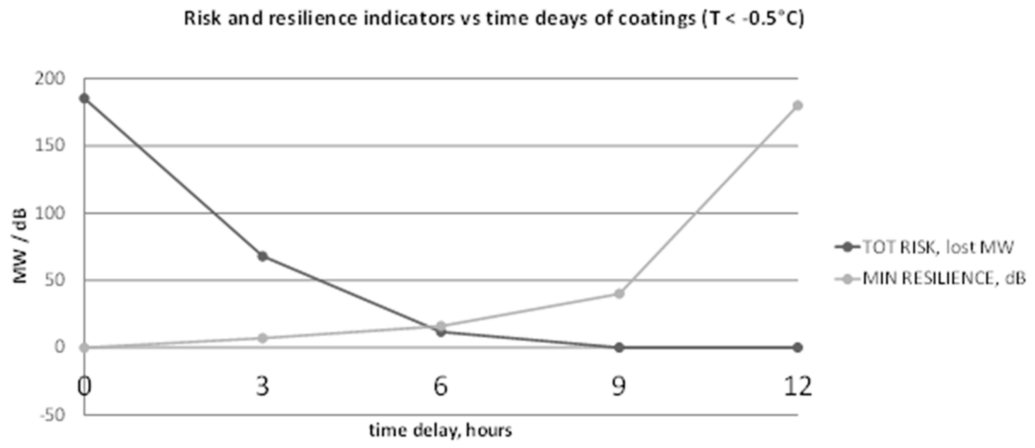
5.5.3. Effect of Hydrophobic Coatings (EM1-C and EM2-C Cases)

This subsection describes an engineering mode application to the same GRID 1 model, and it simulates the deployment of hydrophobic coatings to the critical lines identified by base cases EM1 and EM2. Simulations are run for four values (3, 6, 9, and 12) of the time delays TLIM, in hours, assured by the coatings, assuming an air temperature of −0.6 °C.

For the severe storm (EM1 and EM1-C), Figure 10 shows the total LOL risk and the system resilience indicator (in dB with base level 10⁻²) accounting for different time delays (from 3 to 12 h).

It is worth noticing that a 3 h delay already decreases the total LOL risk by 60%; with a 9 h delay the risk reaches a very low value. Simulations on moderate storm scenarios indicate that a significant enhancement of system resilience can be obtained with a 6 h time delay: Using a 9 h time delay determines only a limited improvement of resilience.

5.5.4. Effect of Generation Redispatching (EM1-A, EM2-A Cases)

Generation redispatching may represent an interesting active measure to enhance the power system resilience to wet snow by assuring a minimum anti-icing current on 230/400 kV lines. However, it may be less effective on 132 kV lines because 132 kV grids are usually operated with few generators and the sensitivity on HV line power flows of generators belonging to the EHV grid is largely limited by the impedance of EHV/HV transformers. Table 5 has showed that all the most critical lines are 132 kV lines in cases EM1 and EM2. However, some 220 and 400 kV lines have a not negligible failure probability due to wet snow sleeve formation. In this case, the minimum current constraints refer only to the 230/400 kV lines which show failure probabilities higher than 5% in base cases EM1 and EM2: Even if their failure probabilities are relatively low, the loss of these lines generally determine very larger variations of power flows with respect to 132 kV lines.

For 132 kV lines, other measures like coatings can effectively reduce the risk of outage, as reported in the previous subsections; accordingly, an effective increase of power system resilience can be obtained by combining two or more measures.

In case EM1-A (severe storm and redispatching), if one assumes a penalization factor for grid losses [29] equal to 10, simulations indicate a redispatched power equal to 8675 MW and an overall redispatching cost equal to 9.10 × 10⁵ arbitrary monetary units (a.m.u.). This large cost is in a few hours is explained by the large social, economic impact that these events would have.

Table 7. Initial, final, anti-icing currents for the critical branches—EM1-A and EM2-A cases.

Severe Storm—EM1-A
Branch ID	Initial Current, A	Final Current, A	Anti-Icing Current Requirement, A
VLVR–TERR	345	920.7	1990
MONR–VLLR	89	467.9	582
PRVR–SGIR	54	144.5	663
Moderate Storm—EM2-A
Branch ID	Initial Current, A	Final Current, A	Anti-Icing Current Requirement, A
PR2R–SGIR	38	301.1	300.1
PRVR–SGIR	54	132.0	300.1

reports the initial, final currents and the anti-icing requirements on the critical lines for cases EM1-A and EM2-A. The current of line MONR-VLLR reaches 467 A, superior to the alarm level set at the TSO control center, i.e., 70% of the minimum anti-icing current (70% × 582 A = 407.4 A). If one considers line PRVR-SGIR connecting PRVR power plant to the rest of 220 kV grid, the maximum active power generation of the unit (50 MW) is not sufficient to attain the minimum anti-icing requirement in cases EM1-A and EM2-A. This represents an intrinsic limit of the measure: It is often ineffective in case of branches which connect single power plants (or load centers) to the rest of the grid.

In presence of moderate wet snow events (case EM2-A) the two affected 220 kV lines are near PRVR power plant and the minimum anti-icing current for both is 300.1 A, higher than the initial currents in the base case, but smaller than the anti–icing requirements for severe events.

These results are obtained with a total redispatched generation equal to 1837.2 MW and a total cost of 1.92 × 10⁵ a.m.u.: The measure effectively prevents wet snow sleeves from accreting on line PR2R – SGIR in moderate events (EM2-A).

5.5.5. The Base Cases of the T&D Grid (EM3 and EM4) for Wet Snow Scenarios

Wet snow storms of the same intensity as previous events S1 and S2 are applied to GRID 2 model which contains both two MV feeders and a portion of the HV grid connected to these feeders. For all the overhead conductors in MV and HV grids Figure 11a reports the expected values of the stress variables (i.e., the mechanical tension) on the conductors, and the loads due to wet snow and wind, in case EM4 of moderate wet snow.

Figure 11b reports the contributions to the total LOL risk for moderate wet snow storm (case EM4) of each contingency category. The largest contributions to the total risk are associated to high order common mode branch outages (N-13 and N-14): In fact, most of the selected critical lines have a very high probability of failure.

In the severe wet snow base (EM3) the set of most critical components includes 52 critical branches, of which 37 have a failure probability higher than 90% and 15 a failure probability between 0.9 and 0.1.

The severe event causes very high probability of damage not only on small section branches (35 mm²) section but also on main branches of the MV network (such as 40–41) with higher sections (70 mm²). The risk of damages on a very large set of branches (up to 52) is much higher than in case EM4.

5.5.6. Effect of Active Measures (EM3-A1 and EM4-A2) for Wet Snow Scenarios

Case EM3-A1 simulates the optimal reconfiguration algorithm to the N-2 outage of branches 40–41 and 16–19 found as a risky contingency in case EM3 which determines the LOL of several customers connected to the Rhemes Valley feeder.

Table 8. Performance indicators for different counterfeed reconfigurations, outage of branches 40–41 and 16–19.

State	MV	Percentage of Restored Load (%)	plosses, MW
001	0.9951	66.67	0.0119
010	0.9987	48.30	0.0087
100	0.997	81.63	0.0125
011	0.9951	66.67	0.0119
101	0.9951	100	0.0156
110	0.9975	81.63	0.0109

reports the minimum MV voltage (M_V), the percentage of restored load and the active power losses (p_losses) obtained after applying any combinations of one or two switching actions: There is no “one switching” reconfiguration of a counterfeed (k = 1) which allows a full restoration of the disconnected load.

The optimal reconfiguration algorithm looks at all the reconfigurations of two counterfeeds (k = 2). Only one reconfiguration with k = 2, (i.e., X_63–26 = 1, X_26–31 = 0 e X_12–46 = 1), allows restoring the unsupplied load with a minimum number of maneuvers, preserving also the radiality of the post-contingency network topology.

In case EM4-A2 the OPF measure is applied on branch #53–#57 with a rated current of 70A, to attain increasing requirements in terms of minimum anti-icing current. The application of the minimum current constraint determines changes in typical network operating quantities such as high power counter-flows, low voltage at extreme branch node and on Primary Substation (PS) MV busbar (through OLTC tap position) as shown in

Table 9. Network power flows in the analysed branch for different minimum current values.

Minimum Current Value (A)	#53–#57 Active Power (kW)	#53–#57 Reactive Power (kVar)	#57 Voltage (p.u.)	PS MV Busbar Voltage at Primary Substation
0	−282	−126	0.968	0.965
25	27	−701	0.964	0.961
70	1827	−116	1.010	0.990

.

5.5.7. Effect of Passive Measures (EM3-P1 and EM4-P2) for Wet Snow Scenarios

Case EM4-P2 considers the reconductoring of some small section conductors. The OHLs with a 35 mm² section found to be critical in base case EM4 are upgraded: Their section areas pass from 35 mm² to 70 mm². This noticeably limits the failure probability of critical components (the highest failure probability is 7.15 × 10⁻¹). The total LOL risk over 10 min passes from 1.33 expected lost MW in the base case to 0.72 expected lost MW in the present case.

The construction of the new counterfeed in case EM3-P1 only slightly decreases the total LOL risk over the whole set of contingencies but significantly reduces the impact for a set of about 20 contingencies. Figure 12 shows the LOL impact of these contingencies before and after the application of this measure.

The highest reduction of LOL is identified for the busbar contingencies affecting nodes 64 thru 90 along the feeder in Valsavarenche valley which also includes the terminals of the counterfeed i.e., nodes 48 and 91. On the contrary, high order N-k contingencies cause very large disruptions that the activation of a single counterfeed cannot reduce the LOL due to the contingency [37].

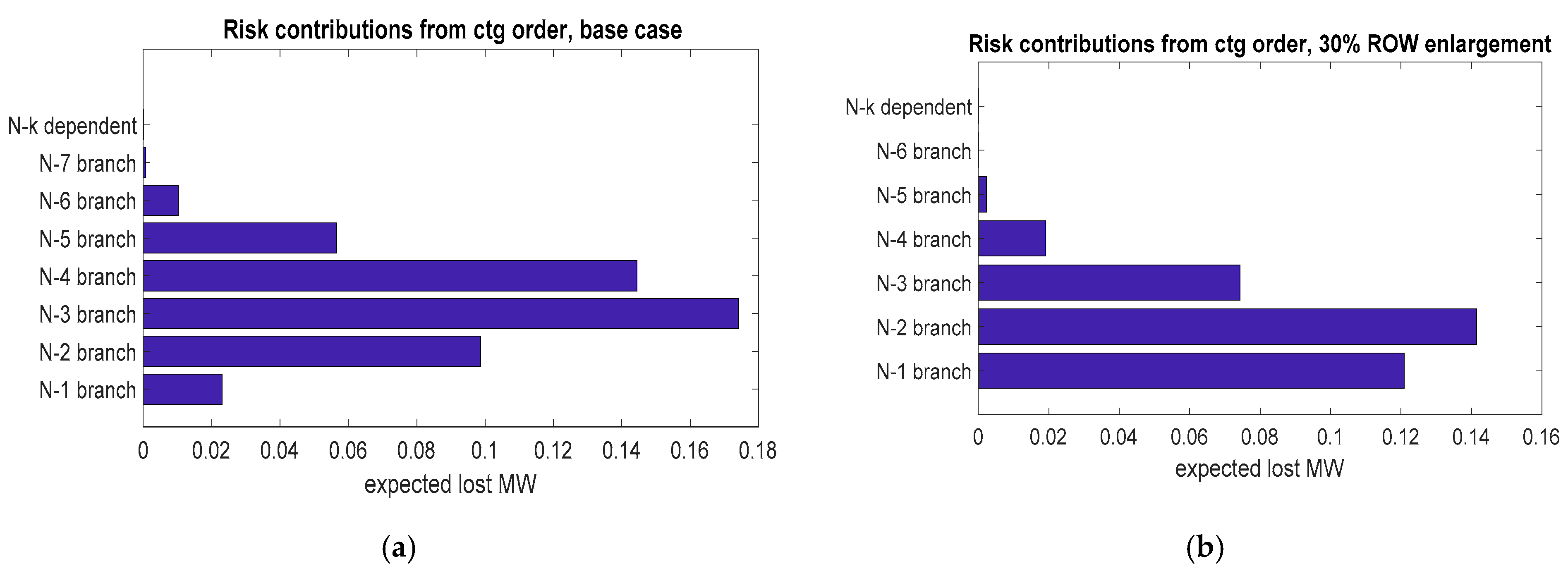
5.5.8. Tree Fall Scenarios for T&D Grid: Base Case (EM5) and Application of Passive Measures (EM5-P1 and EM5-P2)

In base case EM5, RELIEF identifies 7 critical lines, i.e., the lines more prone to fail due to tree contact. CORINE database [41] has been used to derive the data about tree coverage in the area.

All of these critical lines are MV lines which are more affected than HV lines by tree contacts due to their smaller size. These MV lines all belong to the “Val Savarenche” feeder: The risk of tree fall in this zone is also reported in the resilience plan of DEVAL, the local DSO, [38] which proposes the construction of an underground cable to increase the resilience of the area. This good matching obtained using only standard design criteria for the lines and public data demonstrates the relatively low sensitivity of the model to the specific choice of parameters, provided that reasonable ranges of parameter values are considered. The set of most risky contingencies involving the critical lines includes N-1 branch outages, N-k common mode branch outages, and N-k busbar dependent contingencies which lead to a total LOL risk indicator of 0.508. Figure 13a reports the absolute contribution to the risk of load disruption for each contingency category. The largest contributions to the overall LOL risk are due from multiple common mode branch contingencies, also characterized by the largest median impact indicator (around 0.6 lost MW). Relatively low-order contingencies (e.g., N-2) can have high median LOL impacts due to the absence of a counterfeed which can take over the end section of the Val Savarenche feeder. This confirms the need for the underground cable explained in [38].

Case EM5-P1 simulates an enlargement of the ROW width by 30% with respect to standard TSO practices. This measure decreases the number of critical lines from 7 to 6; however, the failure probabilities of the critical lines decrease only by a relatively low amount, because the trees of the dominant species (i.e., larches) have a height up to 30 m and generally the ROW assigned to MV lines is relatively small (around 15–20 m). From Figure 13b it can be noticed that the total LOL risk passes from 0.508 to 0.358 expected lost MW’s (30% reduction), of which the largest contributions are due to N-k common mode branch outages. In this case, a 30% enlargement is not sufficient if the trees outside the ROW are not properly trimmed [28].

To demonstrate the effect of trimming, case EM5-P2 assumes that the trimming policy changes in the utility: The ROW is kept the same as in the base case but a more frequent trimming is applied so that the expected height for trees just outside the ROW is kept at 10 m. This measure leads to the absence of critical lines.

6. Conclusions

The paper has presented an innovative methodological framework to quantify the benefits to resilience brought by resilience boosting measures over different time frames (from long term grid planning to operational planning), which is performed thanks to the mathematical modeling of many measures from anti-torsional devices and superhydrophobic coatings to active measures such as contingency forecasting or optimal power flow based redispatching of generators or optimal reconfiguration actions. The methodology flexibility in modeling different threats (e.g., wet snow tree fall and pollution) and the physical vulnerability of the components makes it suitable to perform “what if” analyses, comparing different technologies for grid hardening. Simulations carried out on realistic models of T&D systems demonstrate the capability of the RSE methodology to easily model and simulate different hardening and smart solutions, which is a fundamental step for the quantification of their benefits expressed as the reduction of load disruption risk, in case of different severities and extents of the weather threats.

Ongoing work consists in exploiting the models developed for resilience boosting measures within an optimization framework to identify the optimal set of active and passive measures to enhance resilience over different time frames from long term planning to real time operation.

References

1. Panteli, M.; Mancarella, P. Influence of extreme weather and climate change on the resilience of power systems: Impacts and possible mitigation strategies. Electr. Power Syst. Res. 2015, 127, 1–30. [Google Scholar] [CrossRef]
2. Panteli, M.; Mancarella, P.; Trakas, D.N.; Kyriakides, E.; Hatziargyriou, N.D. Metrics and quantification of operational and infrastructure resilience in power systems. IEEE Trans. Power Syst. 2017, 32, 4732–4742. [Google Scholar] [CrossRef] [Green Version]
3. Agency for the Cooperation of Energy Regulators (ACER). European Energy Regulation: A Bridge to 2025. Green Paper; Agency for the Cooperation of Energy Regulators: Ljubljana, Slovenia, 2014. [Google Scholar]
4. Javanbakht, P.; Mohagheghi, S. Mitigation of snowstorm risks on power transmission systems based on optimal generation re-dispatch. In Proceedings of the of 2016 North American Power Symposium (NAPS), Denver, CO, USA, 18–20 September 2016; pp. 1–5. [Google Scholar]
5. Kezunovic, M.; Obradovic, Z.; Dokic, T.; Zhang, B.; Stojanovic, J.; Dehghanian, P.; Chen, P.-C. Predicating spatiotemporal impacts of weather on power systems using big data science. In Data Science and Big Data: An Environment of Computational Intelligence; Springer: Dusseldorf, Germany, 2017; ISBN 978-3-319-53474-9. [Google Scholar]
6. Tin, P.; Zin, T.T.; Toriu, T.; Hama, H. An integrated framework for disaster event analysis in big data environments. In Proceedings of the 2013 Ninth International Conference on Intelligent Information Hiding and Multimedia Signal Processing, Beijing, China, 16–18 October 2013; pp. 255–258. [Google Scholar]
7. Grolinger, K.; Capretz, M.A.M.; Mezghani, E.; Exposito, E. Knowledge as a service framework for Disaster data management. In Proceedings of the Workshop on Enabling Technologies: Infrastructure for Collaborative Enterprises, Hammamet, Tunisia, 17–20 June 2013; pp. 313–318. [Google Scholar]
8. Wang, Y.F.; Deng, M.H.; Bao, Y.K.; Zhang, H.; Chen, J.Y.; Qian, J.; Guo, C.X. Power system disaster-mitigating dispatch platform based on big data. In Proceedings of the International Conference on Power System Technology, Chengdu, China, 20–22 October 2014; pp. 1014–1019. [Google Scholar]
9. Chen, L.; Chao, Y.; Ma, Y. Risk warning system based on big data applied in the power informatization of state grid. In Proceedings of the 3rd International Conference on Information Science and Control Engineering (ICISCE), Beijing, China, 8–10 July 2016; pp. 578–582. [Google Scholar]
10. Chen, P.C.; Kezunovic, M. Fuzzy logic approach to predictive risk analysis in distribution outage management. IEEE Trans. Smart Grid 2016, 7, 2827–2836. [Google Scholar] [CrossRef]
11. Bonelli, P.; Lacavalla, M.; Marcacci, P.; Mariani, G.; Stella, G. Wet snow hazard for power lines: A forecast and alert system applied in Italy. Nat. Hazards Earth Syst. Sci. 2010, 11, 2419–2431. [Google Scholar] [CrossRef]
12. Ciapessoni, E.; Cirio, D.; Pitto, A.; Van Harte, M.; Panteli, M.; Mak, C. Defining power system resilience. Electra CIGRE J. 2019, 306, 32–34. [Google Scholar]
13. CIGRE WG C1.27. The Future of Reliability—Definition of Reliability in Light of New Developments in Various Devices and Services which Offer Customers and System Operators New Levels of Flexibility; Technical Brochure 715; CIGRE: Paris, France, 2018. [Google Scholar]
14. FERC. Comments of the North American Electric Reliability Corporation; FERC: Washington, DC, USA, 2018. [Google Scholar]
15. NERC. State of Reliability; Technical Report; NERC: Atlanta, GA, USA, 2017. [Google Scholar]
16. NERC. Definition: Adequate Level of Reliability for the Bulk Electric System, March 2013. Available online: https://www.nerc.com/ (accessed on 20 June 2019).
17. Singh, C. Is Resilience Different from Reliability? Available online: http://chanansingh.engr.tamu.edu/wp-content/uploads/sites/199/2018/10/Resilience-and-reliability-2.pdf (accessed on 20 June 2019).
18. Yong, L.; Singh, C. A methodology for evaluation of hurricane impact on composite power system reliability. IEEE Trans. Power Syst. 2011, 26, 145–152. [Google Scholar]
19. Clark-Ginsberg, A. What’s the Difference between Reliability and Resilience? Available online: https://www.researchgate.net/publication/320456274_What’s_the_Difference_between_Reliability_and_Resilience (accessed on 20 June 2019).
20. Ciapessoni, E.; Cirio, D.; Kjølle, G.; Massucco, S.; Pitto, A.; Sforna, M. Probabilistic risk-based security assessment of power systems considering incumbent threats and uncertainties. IEEE Trans. Smart Grid 2016, 7, 2890–2903. [Google Scholar] [CrossRef]
21. Ni, M.; McCalley, J.D.; Vittal, V.; Tayyib, T. Online Risk-Based Security Assessment. IEEE Trans. PS 2003, 18, 258–265. [Google Scholar] [CrossRef]
22. Ciapessoni, E.; Cirio, D.; Pitto, A.; Sforna, M. A quantitative methodology to assess the process of service and infrastructure recovery in power systems. In Proceedings of the 2020 PSCC Conference, Porto, Portugal, 28–3 July 2020. [Google Scholar]
23. Ciapessoni, E.; Cirio, D.; Pitto, A.; Sforna, M. A probabilistic risk-based security assessment tool allowing contingency forecasting. In Proceedings of the PMAPS 2018 Conference, Boise, ID, USA, 24–28 June 2018. [Google Scholar]
24. Ciapessoni, E.; Cirio, D.; Pitto, A.; Pirovano, G.; Sforna, M. Analytical modelling of overhead line vulnerability to wet snow events for resilience assessment. In Proceedings of the AEIT International Conference, Florence, Italy, 18–20 September 2019. [Google Scholar]
25. Freddo, A.; Ottino, G.; Posati, A.; Rebolini, M.; Bonelli, P.; Golinelli, E.; Lacavalla, M.; Marcacci, P.; Perini, U.; Pirovano, G. Wet–snow accretion on conductors: The Italian approach to reduce risks on existing OHL. In Proceedings of the CIGRE Session, Paris, France, 26–31 August 2012. [Google Scholar]
26. ISO/TC98/SC3/WG6. Atmospheric Icing of Structures; International Standard, ISO 12494; ISO: Geneva, Switzerland, 2000. [Google Scholar]
27. Ciapessoni, E.; Cirio, D.; Pitto, A.; Pirovano, G.; Sforna, M. A risk-based resilience assessment tool to anticipate critical system conditions in case of natural threats. In Proceedings of the Powertech 2019 Conference, Milan, Italy, 23–27 June 2019. [Google Scholar]
28. Ciapessoni, E.; Cirio, D.; Pitto, A.; Pirovano, G.; Sforna, M. Modelling the vulnerability of overhead lines against tree contacts for resilience assessment. In Proceedings of the PMAPS 2020 Conference, Liege, Belgium, 18–21 August 2020. [Google Scholar]
29. Ciapessoni, E.; Cirio, D.; Pitto, A.; Marcacci, P.; Sforna, M. Security-constrained redispatching to enhance power system resilience in case of wet snow events. In Proceedings of the PSCC 2018 Conference, Dublin, Ireland, 11–14 June 2018. [Google Scholar]
30. Carlini, C.; Ciapessoni, E.; Cirio, D.; Marcacci, P.; Moneta, D.; Pitto, A. Resilience assessment and enhancement in electric distribution networks. In Proceedings of the IWAIS 2019 Conference, Rejikiavik, Iceland, 23–28 June 2019. [Google Scholar]
31. Yuan, C.; Illindala, M.S.; Khalsa, A.S. Modified Viterbi Algorithm based distribution system restoration strategy for grid resiliency. IEEE Trans. Power Deliv. 2017, 32, 310–319. [Google Scholar] [CrossRef] [Green Version]
32. Admirat, P.; Lepeyre, J.L. Theoretical study and experimental verification of the torsion of cables subjected to moment densities. In Proceedings of the 4th IWAIS Conference, Paris, France, January 1988. [Google Scholar]
33. Chemelli, C.; Ciapessoni, E.; Cirio, D.; Marcacci, P.; Pirovano, G.; Pitto, A.; Massucco, S.; Sforna, M. Quantifying benefits of grid reinforcement measures to power system resilience against wet snow events. In Proceedings of the 2019 ISGT Europe Conference 2019, Bucharest, Romania, 29 September–2 October 2019. [Google Scholar]
34. Januja, Z.A. The Influence of freezing and ambient temperature on the adhesion strength of ice. In Cold Region Science and Technology; Elsevier: Amsterdam, The Netherlands, 2017; Volume 140, pp. 14–19. [Google Scholar]
35. Chen, T.; Cong, Q.; Sun, C.; Jin, J.; Choy, K.-L. Influence of substrate initial temperature on adhesion strength of ice on aluminium alloy. In Cold Regions Science and Technology; Elsevier: Amsterdam, The Netherlands, 2018; Volume 148, pp. 142–147. [Google Scholar]
36. Xinbo, H. The effect of surface roughness on heat transfer coefficient. In Proceedings of the IWAIS 2017, Chongqing, China, 24–29 September 2017. [Google Scholar]
37. Ciapessoni, E.; Cirio, D.; Moneta, D.; Pitto, A.; Carlini, C. Comprehensive risk based methodology and tool for a quantitative resilience assessment of distribution and transmission systems. In Proceedings of the CIRED 2019, Madrid, Spain, 3–6 June 2019. [Google Scholar]
38. DEVAL. Resilience Plan 2019–2021. Addendum to Development Plan 2019–2021; DEVAL: Aosta, Italy, 2018. (In Italian) [Google Scholar]
39. CENELEC Std. EN 50341-2-13:2017-01. Overhead Electrical Lines Exceeding AC 1 kV—Part 2-13: National Normative Aspects (NNA) for Italy (Based on EN50341-1:2012); CENELEC: Brussels, Belgium, 2017. [Google Scholar]
40. Engelbrecht, C. A simplified statistical method for the qualification of insulators for polluted environments. In Proceedings of the 2002 CIGRE Session, Paris, France, 25–30 August 2002. [Google Scholar]
41. CORINE Database. Available online: https://land.copernicus.eu/pan-european/corine-land-cover/ (accessed on 15 September 2019).
Figure 1. Model of relationship between reliability and resilience: resilience as a third subproperty of reliability.
Applsci 10 05402 g001
Figure 2. The bow tie model.
Applsci 10 05402 g002
Figure 3. Conceptual relationship among the variables derived from the bow tie.
Applsci 10 05402 g003
Figure 4. (a) List of overhead lines (OHLs) with increasing RPs—EN 50341 indications for extreme values distribution, (b) Georeferenced map of OHLs with colors indicating increasing values of return periods (from magenta to white)—extreme values evaluated via Std EN 50341-2-13.
Applsci 10 05402 g004
Figure 5. Profile of return periods (RPs) for OHLs in case of insulators design for (a) heavy pollution, (b) very heavy pollution, and (c) exceptional pollution.
Applsci 10 05402 g005
Figure 6. Profile of RPs for grid components (other than OHLs) in case of insulators design for (a) heavy pollution, (b) very heavy pollution, and (c) exceptional pollution.
Applsci 10 05402 g006
Figure 7. Ice thickness in mm (top right diagram), mechanical tension (top left diagram) and mechanical load on tower equipment in kN (bottom left diagram) in the first 10 h of the forecasting interval.
Applsci 10 05402 g007
Figure 8. Geolocalization of critical components for severe wet snow (a) and moderate wet snow storm (b).
Applsci 10 05402 g008
Figure 9. Risk of loss of load (LOL) for severe (S1) and moderate (S2) storm scenarios, and two different inter-device distances—cases EM1, EM1-T, EM2, and EM2-T.
Applsci 10 05402 g009
Figure 10. Risk and resilience metrics for different time delays for severe storm (EM1 and EM1-C).
Applsci 10 05402 g010
Figure 11. (a) Mechanical tension in kN for medium voltage (MV) MV and high voltage (HV) lines, (b) Contributions to total risk of each contingency category, case EM4.
Applsci 10 05402 g011
Figure 12. Bar diagram of the LOL impact of the contingencies before and after the new counterfeed, severe wet snow event EM3-P1.
Applsci 10 05402 g012
Figure 13. Contributions of each contingency category to the overall LOL risk in expected lost MW (a) in base case EM5, and (b) in case of 130% ROW (EM5-P1).
Applsci 10 05402 g013