A Novel Framework for Synchrophasor Based Online Recognition and Efficient Post-Mortem Analysis of Disturbances in Power Systems

Featured Application

Synchrophasor based data compression and post-mortem analysis as well as online detection and classification of grid disturbances.

Abstract

Synchrophasor based applications become more and more popular in today’s control centers to monitor and control transient system events. This can ensure secure system operation when dealing with bidirectional power flows, diminishing reserves and an increased number of active grid components. Today’s synchrophasor applications provide a lot of additional information about the dynamic system behavior but without significant improvement of the system operation due to the lack of interpretable and condensed results as well as missing integration into existing decision-making processes. This study presents a holistic framework for novel machine learning based applications analyzing both historical as well as online synchrophasor data streams. Different methods from dimension reduction, anomaly detection as well as time series classification are used to automatically detect disturbances combined with a web-based online visualization tool. This enables automated decision-making processes in control centers to mitigate critical system states and to ensure secure system operations (e.g., by activating curate actions). Measurement and simulation-based results are presented to evaluate the proposed synchrophasor application modules for different use cases at the transmission and distribution level.

1. Introduction

The electrical power system is in a transition process. While the number of converter-interfaced renewable generation rises, conventional power plants are decommissioned, which leads to a reduced system inertia and rises volatility in the electrical power system [1,2]. The deregulation of electricity generation and unbundling of the market from transmission and distribution tasks introduces additional challenges [3]. Thus, today’s control room operators are facing a large number of events during daily system operation. To address these challenges, synchronized phasor measurements and wide area monitoring (WAM) systems are deployed worldwide in power system control rooms [4]. Being a valuable resource to observe and understand the dynamics of power systems, they additionally enable a new quality of operator decision support functions, assistant systems and automated control [4,5,6]. This study presents a novel framework of machine learning-based applications for analyzing historical and online synchrophasor measurements. This enables the efficient processing and post-mortem analysis of large, unlabeled measurement records as well as the online detection and classification of grid disturbances in an automated fashion. The interaction of these novel applications as well as the online visualization of the results allow an enhanced situational awareness for the recognition and assessment of critical system states and the activation of appropriate counter measures to ensure a secure system operation. Chapter 2 presents a state of the art for synchrophasor applications, their current usage in today’s power systems as well as limitations for a widespread utilization. Following a literature review of recent research fields in Section 2.3, the novel framework for advanced synchrophasor applications is presented in Section 3.1. Section 3.2 and Section 3.3 describe the offline applications spatiotemporal data compression module and disturbance extraction module and Section 3.4 and Section 3.5 follow with detailed descriptions of the disturbance detection module and disturbance classification module. Section 4 presents and discusses the application results from different case studies including field measurements as well as dynamic grid simulations. A short presentation of a web-based visualization tool is given in Section 5. Section 6 concludes the investigations and gives a short outlook for possible future work.

2. Synchrophasor Technology and State of the Art Applications

2.1. Application of Synchrophasors in Modern Control Centers

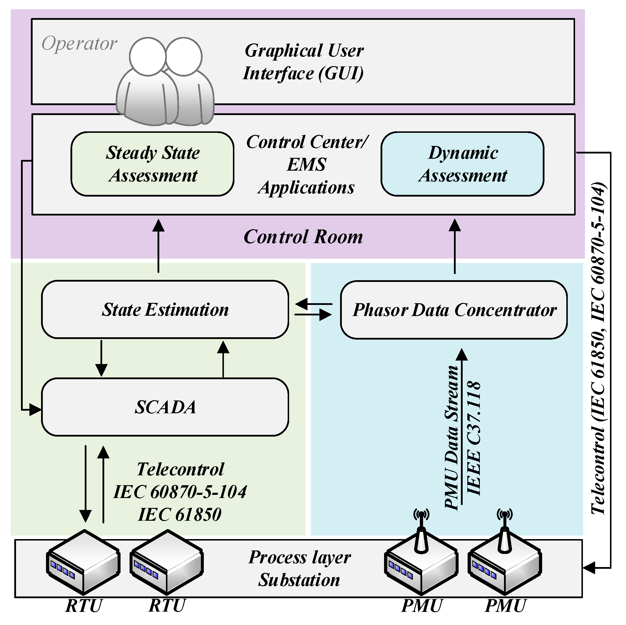
Conventional supervisory control and data acquisition (SCADA) systems do not provide the ability to monitor transient events [7,8]. Even though the connected remote terminal units (RTU) can communicate cyclically, the measurements samples are typically not time aligned when arriving at the control center [9,10]. Thus, a state estimator is required [9]. Unless a general interrogation is inquired, traditional SCADA protocols (e.g., IEC 60870-5-101 /-104 [11] and DNP3 [12]) only transmit spontaneous messages in case of measurement value changes or if a switch status message has been received. This requires a state estimation (SE) to generate a valid steady-state power flow image of the system state. This state estimate is used by most secondary energy management system (EMS) functions and applications (i.e., contingency analysis, optimization, etc.); hence the SE module is often referred to as the cornerstone of an EMS. Dynamic stability assessment (DSA) systems can enhance the situational awareness in transmission control centers significantly [13]. DSA systems run time-domain simulations to evaluate possible contingencies as well as suitable mitigation strategies. These results can also be used for the creation of training sets for machine learning based analysis modules. Additionally, phasor measurement unit (PMU) based wide area monitoring (WAM) systems increase the dynamic observability by recording transient events by time synchronized samples. The synchronization accuracy of modern GPS linked PMUs is below 1µs [14]. Modern phasor data concentrators (PDC) can acquire data from several hundred PMUs [15,16,17]. An IEEE C37.118 [18] conform interface to IEC 61850 [19] is available, which increases the flexibility of PMU data processing [20]. The synthetic patterns created by DSA systems and the recorded patterns from WAMS can be used to improve the training set as well as the DSA time-domain model. A promising application is the HVDC based RAS, an automated control strategy to exploit the flexibility of the VSC technology to substitute the expensive generator-based redispatch [21].

Today’s synchrophasor applications typically run in parallel to existing SCADA based control room applications (see Figure 1). According to [22], common PMU applications can be distinguished into real-time operation tasks (e.g., frequency stability monitoring, power oscillation monitoring, phasor-only state estimation, dynamic line rating) and planning tasks (e.g., model calibration, primary frequency response analysis, post-mortem analysis). Further applications as well as possible enhancements of SCADA based monitoring and control applications were also investigated in [23,24]. A recent study identified the following hindering issues for a wider application of synchrophasor technology in today’s system operation [25]:

• A clear determination of accurate, dynamic operating limits (i.e., phase-angle differences, or oscillations) is not available, which diminishes the value of the information gain for the system operation.
• The data quality still strongly depends on the quality of the instrument transformers, as well as the ICT infrastructure.
• The rising observability due to a newly installed WAMS can lead to an exposition of new issues, which can lead to a commitment of valuable personnel to investigate the problems.
• Unless some TSOs exchange data of strategic important PMUs, the data exchange is often subject to cyber security issues or other sensitivities.
• A separate development of EMS and WAMS lead to challenges for human operators, who prefer a single unified user interface to support a smoother workflow and a clear decision-making.
• A general evaluation scheme of system dynamics and correlating actions still needs to be defined.
• An operator training, addressing the understanding and the interpretation of dynamic phenomena, needs to be established to raise the level of operator awareness and to establish a flexible response to events, instead of a mainly rule-based operation.

2.2. Enhanced Situational Awareness

The most commonly used definition of situation awareness (SA) describes it as “the perception of the elements in the environment within a volume of time and space, the comprehension of their meaning, and the projection of their status in the near future” [26]. As the complexity of the power system operation grows, the risk of human induced errors with consequences for the system security will rise. In future, human operators need appropriate tools to assist their cognitive capabilities in the evaluation of a growing amount of data gathered in the control room for a quicker diagnosis and decision-making [27]. Assistance systems can enhance the SA during the system operation and allows to perceive critical situations earlier.

2.3. State of the Art Analysis of Synchrophasor Based Detection and Mitigation of Critical Events

Current research in the field of synchrophasor based applications for enhanced monitoring and control mainly focus on online or real-time methods. This includes robust statistical or machine learning based algorithms for the automated detection, localization and identification of critical events or cascading events [28,29,30]. Online algorithms for the automated detection or assessment of system instabilities (e.g., by computing stability margins), like transient and small signal stability, were introduced in [31,32]. Apart from recognition tasks, authors in [33,34,35] suggest the utilization of PMUs for the real-time control of active grid components (e.g., for damping of inter-area oscillations or activating special protection schemes) as part of a wide area monitoring, protection and control (WAMPAC) system. This also enables a synchrophasor based congestion or restoration management including suitable monitoring and control algorithms. In addition to the use of PMUs in transmission power systems, authors in [36,37] investigated the application of low-cost µ-PMUs for lower voltage levels (distribution grids). The automated detection of grid disturbances and the activation of suitable countermeasures (e.g., curative actions) is an important application to prevent or mitigate major supply disruptions or blackouts. It enables a fast and reliable system operation with reduced human supervision. Existing approaches for the online detection, identification, and localization of grid disturbances from synchrophasor measurements utilize different feature extraction and classification techniques. Additionally, there are major differences with regard to the addressed task (detection, identification or localization), the investigated contingency events and the used input data (e.g., measurement channels, pre- and post-disturbance time). Authors in [38] propose a simple k-Nearest Neighbor based method to detect different events from its oscillation modes using frequency measurements. More sophisticated approaches utilize support-vector machines [39] or decision rules [40] to identify different disturbance events voltage spikes, load losses or line trips. The combined identification and localization (disturbance classification) of different line trip and short circuit events is investigated in [28,41] by analyzing voltage signals. Other works use frequency and voltage measurements to classify various disturbance events by combining wavelets and support vector machines [42,43] or S-Transforms and extreme learning machines [30]. The disturbance classification, as a supervised learning task, relies on a sufficient training database with a predefined selection of critical contingencies. The sole generation of a measurement based training dataset using post-mortem analysis is computationally costly, has high risks to incomplete datasets (only observed contingencies can be considered) and requires a large amount of historical phasor measurement records. Most of the studies, therefore, utilize dynamic grid simulations to generate a representative training dataset. This requires a detailed knowledge of the grid topology and the control parameters of the relevant active grid components as well as a suitable simulation tool to perform large scale contingency simulations for a wide range of grid scenarios.

Existing recognition approaches mainly focus on measured or simulated online phasor data streams and neglect potential useful information from historical measurement records. In contrast to that, a combined online and offline analysis framework can improve simulation-based detection methods by utilizing knowledge from historical measurements.

3. Novel Framework for Advanced Synchrophasor Analysis in Modern Control Centres

3.1. Framework Architecture and Analysis Modules

In this study, a novel framework for analyzing historical and online synchrophasor measurements is presented in order to detect and classify grid disturbances and to activate suitable countermeasures. In contrast to existing approaches (see Section 2.3), additional knowledge from historical measurement records can be integrated in order to increase the recognition capabilities and the classification accuracies of the online analysis modules. This framework combines different offline and online synchrophasor applications to enable an efficient analysis and decision-making based on simulated and measured critical events. The proposed analysis modules comprise of a spatiotemporal data compression module, disturbance extraction module, disturbance detection module and disturbance classification module.

The spatiotemporal data compression module eliminates redundant information for an efficient processing and analysis of large historical phasor measurement records. Due to the high reporting rates (typically between 10 and 50 frames per second [18]) and the large number of installed PMU sensors especially in large power grids, high data volumes and transmission rates occur when collecting synchrophasor data in control centers. With the use of statistical methods, the storage demand in modern control centers can be drastically reduced. This enables a long-term archiving of phasor data as well as an efficient post-mortem analysis of large datasets. A detailed description of the spatiotemporal data compression module is given in Section 3.2.

The disturbance extraction module analyzes compressed synchrophasor data records to extract potential critical events and to enhance the training database of the disturbance classification module. For this purpose, an intelligent analysis procedure is proposed to automatically explore historical measurement records and to discover potential interesting events that were not detected with existing grid monitoring tools. These events mainly include disturbances like malfunctions, outages, oscillations, faults or other unusual deviations from regular grid operation. It is to be expected, that only a small part of the measurement records contain relevant events. Additionally, no prior knowledge is available, which further complicates the recognition task. Extracted events or disturbances can be processed further, e.g., for root-cause event analysis, the assessment of grid assets and the enhancement of training data or subsequent signal analysis algorithms (e.g., for the disturbance detection module and disturbance classification module in Section 3.4 and Section 3.5).

The disturbance detection module detects deviations from steady conditions by computing an anomaly score for each PMU measurement channel. In contrast to the previous application modules, this is done online using a sliding window-based approach. Generally, there is a vast number of possible events or disturbances, which lead to deviations from steady state conditions including outages, short circuits / faults, oscillations or malfunctions. The automated recognition of these events is a basic prerequisite to prevent undesired or unstable system states and to initiate suitable countermeasures. In contrast to the disturbance classification module, an exact identification of the disturbance type or the location of the disturbance origin is not performed. Instead, the goal of the disturbance detection module is to recognize possible disturbances, if only undisturbed system conditions are known. Therefore, the disturbance detection module can act as a trigger for subsequent process analysis or can enhance the training data base.

In case of high anomaly scores, the disturbance classification module estimates the disturbance type and location of the transient event by computing the corresponding probabilities of occurrence. Similar to the disturbance detection module, this is done online by analyzing the current phasor data stream. Compared to traditional SCADA or protection systems, a wide range of possible disturbances can be detected within short time spans (< 1 s) including outages from generators, lines, or renewable energy sources as well as short circuits or load trips. Precise information about the origin and type of the disturbance as well as additional time and frequency analysis information (e.g., oscillation modes, frequency drops) enable the initialization of precise countermeasures (e.g., curative actions) to restore a stable system state. These actions can be precomputed for different disturbances and updated with each new steady state condition. Today’s DSA systems provide sufficient computation options to simulate different contingencies and to select and assess suitable countermeasures [13]. Further descriptions are given in Section 3.6.

For a better understanding, Figure 2 shows the simplified workflow and interaction between the different synchrophasor based online and offline analysis modules. The phasor data concentrator collects the phasor measurements and continuously updates a database. At the same time, the online data stream is forwarded to the online analysis modules. The offline analysis modules can be activated periodically to process a certain amount of historical measurement records. The measurement and analysis results can be visualized with a web-based user interface (see Section 5) and can be transferred to subsequent EMS applications.

3.2. Spatiotemporal Synchrophasor Data Compression

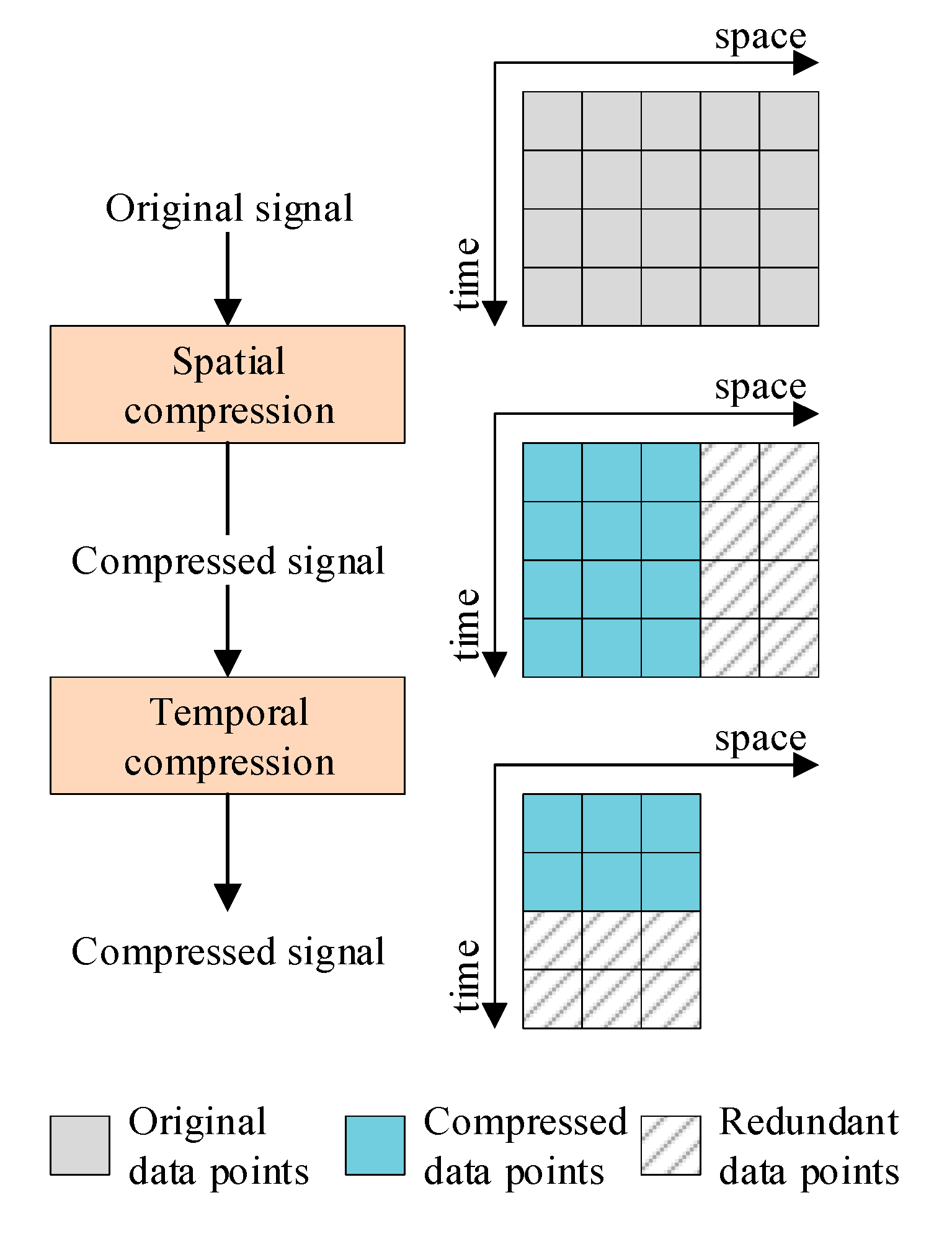
The idea of data compression is to transform the original input measurements into a small subset of coefficients with minimum information loss. The smaller this subset is compared to the size of the uncompressed signal, the higher is the compression rate. The applied signal transformation aims to eliminate all redundant information and can be inverted to reconstruct the original signals with a certain error (reconstruction error). In contrast to existing single-step approaches, the spatiotemporal data compression module combines two compression stages to identify and eliminate redundant synchrophasor data in space (e.g., by PMU sensors with close proximity) and time (e.g., by low signal variations over long time spans)–see Figure 3. This enables high compression rates in presence of transient events and preserves low reconstruction errors. The compression rate $r_{\mathrm{C}}$ is calculated according to (1) given the cardinality of the normalized input signal ${\mathit{X}}_{\mathrm{N}}$ divided by the cardinality of the compressed signal ${\mathit{X}}_{\mathrm{C}}$. The transformation coefficients ${\underset{\_}{\theta }}_{\mathrm{C}}$ must also be taken into account, because they are required to reconstruct the original signals.

$$r_{\mathrm{C}}=\frac{\left|{\mathit{X}}_{\mathrm{N}}\right|}{\left|{\mathit{X}}_{\mathrm{C}}\right|+\left|{\underset{\_}{\theta }}_{\mathrm{C}}\right|}$$

(1)

The reconstruction error $e_{\mathrm{R}}$ is based on the L2-norm (squared Euclidean distance) between the original signal and the reconstructed signal ${\widehat{\mathit{X}}}_{\mathrm{N}}$–see (2).

$$e_{\mathrm{R}}=\Vert {\mathit{X}}_{\mathrm{N}}-{\widehat{\mathit{X}}}_{\mathrm{N}}\Vert$$

(2)

Minimizing this error ensures a close approximation of the original measurement matrix.

For the spatial compression stage, different dimension reduction techniques can be used including principle component analysis (PCA), independent component analysis and non-negative matrix factorization. In case of the temporal compression, time-frequency transformations are suitable like discrete wavelet transform (DWT), discrete cosine transform or fast Fourier transform. Based on preliminary work [44], PCA and DWT are used as best combination to achieve low reconstruction errors and high compression rates. In the spatial compression stage, PCA is applied on the normalized measurement matrix, which creates a set of “virtual” PMU sensors depending on the number of chosen principle components. This ensures that only non-redundant information (highest signal variances) are captured by the first principle components. In this step, the temporal dimension (number of time steps) remains the same. In the second compression stage, DWT transforms each “virtual” sensor signal into the frequency domain. In case of multiple decomposition levels, this transform is applied recursively to generate the approximation and detailed coefficients. A compression is achieved by setting some detailed coefficients to zero depending on a predefined, global threshold value. PCA and DWT are both linear signal transform techniques. The PCA and the DWT parameters can be reused in the spatial and the temporal inverse processes to reconstruct the “virtual” sensor signals as well as the input measurement matrix–see

Table 1. Overview of the data compression techniques and main parameters.

Method	Compression Result	Parameters
PCA	PCA scores (principle components)	PCA loadings, sample means
DWT	approximation and detailed coefficients	low- and high-pass filters, wavelet expansion coefficients

. This procedure is applied on each PMU channel separately assuring optimal compression rates and reconstruction errors. A detailed description of the methodology as well as a comparison between the different compression techniques is given in [44].

3.3. Disturbance Extraction (Post-Mortem Analysis)

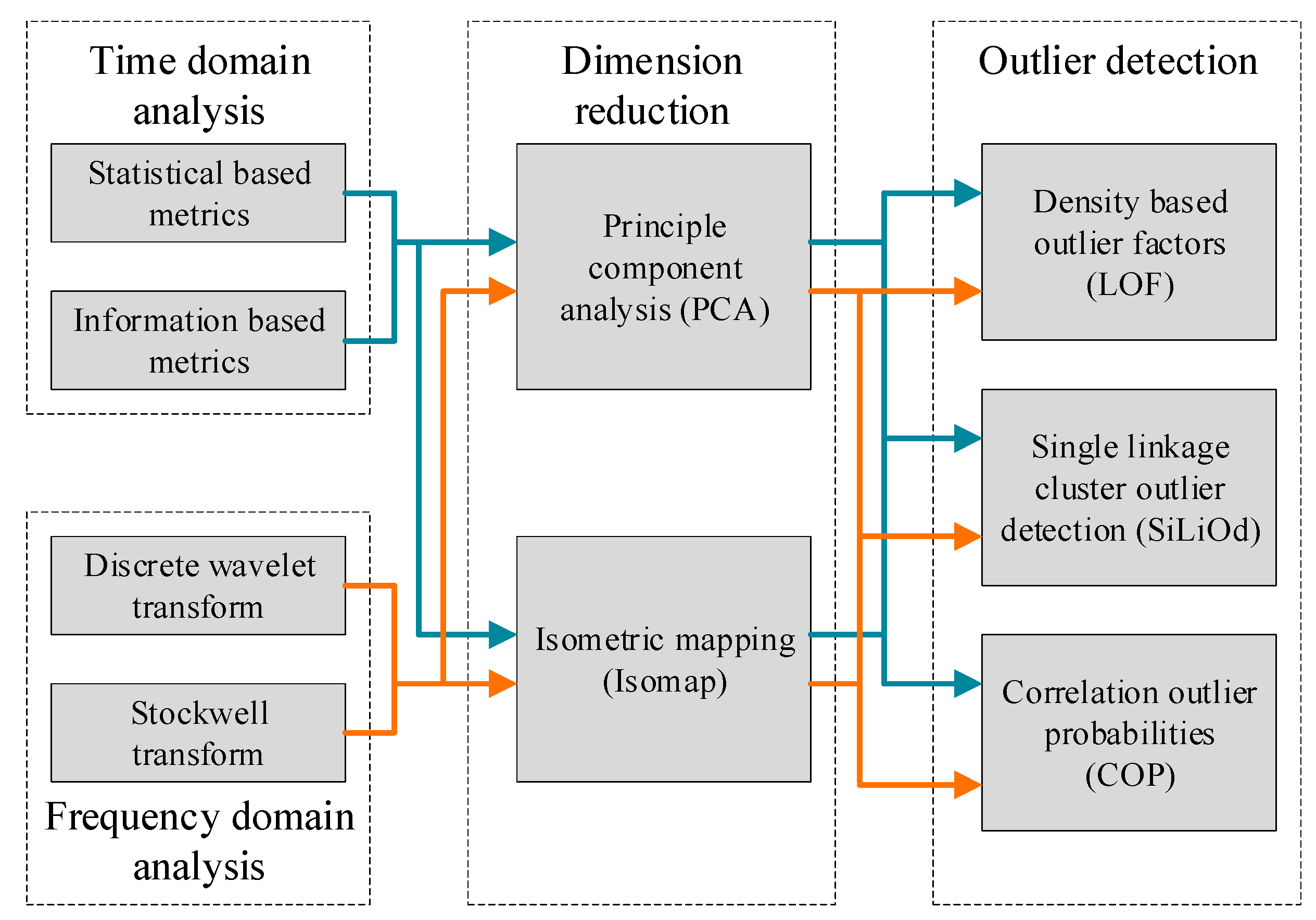
The disturbance extraction module detects a predefined number of possible grid disturbances by analyzing historical records of a single phasor measurement signal (e.g., frequency). The lack of positive examples (non-outliers) and negative examples (outliers) as well as the high diversity of outlier types makes an exact prediction very difficult. To minimize the variance of the model predictions, different feature extraction, dimension reduction and outlier score estimation techniques are combined within an ensemble-based approach. Each outlier detection algorithm uses different metrics for the outlier scores, which makes a direct comparison difficult. Therefore, a rank transformation aggregates the outlier scores of the base detectors, such that high rank values correspond to low outlier scores and vice versa. In a final clustering stage, only the samples with the lowest total rank values are chosen. The goal of the clustering algorithm is to group similar disturbance patterns into meaningful classes. Therefore, a similarity matrix is computed using time-warp edit distance (TWED) [45]. The resulting dissimilarity matrix is passed to a hierarchical density based clustering algorithm (HDBSCAN) [46] to identify the cluster groups without prior knowledge about the number of cluster groups. For the disturbance extraction module, three outlier detection algorithms are used including local outlier factors (LOF) [47], correlation outlier probabilities (COP) [48] and single-linkage based outlier detection (SiLiOd) [49]. These algorithms compute an outlier score to measure the deviation to the normal or majority signal behavior. The main principles of the three algorithms for the outlier scores are given in

Table 2. Overview of the outlier detection techniques and outlier score properties.

Method	Main Principle	Outlier Score
LOF	Local density of data points and its neighborhoods	Local outlier factor
COP	Deviation within local correlation model using robust PCA	Correlation outlier probability
SiLiOd	Hierarchical clustering using shortest distances	Path lengths to final cluster

.

As mentioned earlier, the ensemble-based disturbance extraction module uses multiple base detectors to compute outlier scores and extract potential unusual or abnormal records. The base detectors differentiate with respect to the used dimension reduction technique (PCA or Isomap) and the outlier detection method (LOF, COP or SiLiOd). This leads to a total number of six base detectors within the disturbance extraction module. Each base detector calculates in total 13 features including statistical and information-based metrics in time-domain as well as energy based features from Stockwell transform coefficients and discrete wavelet transform coefficients. This comprehensive feature representation allows to capture various signal traits in different disturbed situations like abrupt signal changes, oscillations, or other dynamic variations. A short overview of the different base detectors is given in Figure 4. Further literature can be found in [49,50].

3.4. Disturbance Detection

Anomaly detection or novelty detection is an active research area in machine learning to automatically detect abnormal signal behavior or signal patterns that deviate strongly from the expected or majority behavior. This is different from the outlier detection (see Section 3.3), in which the negative examples in the training dataset are unlabeled or unknown. Different techniques are proposed in literature including classification based approaches (e.g., one-class support vector machine), clustering based approaches (e.g., density-based clustering) or subspace-based approaches (e.g., principle component analysis) and have a high resemblance with outlier detection methods. Further literature can be found in [51,52]. Compared to other approaches, the z-score based disturbance detection module computes anomaly scores instead of a binary decision. This is done by deriving features in the time- and frequency-domain and by applying a Z-transformation considering a fixed amount of historical feature values. The resulting z-scores are computed for each PMU measurement channel separately assuming a Gaussian feature distribution within the normal grid operation. The basic workflow is given in Figure 5.

The input matrix $\mathit{X}$ consists of the $N$ last measurement samples ${\underset{\_}{x}}^n$ and are normalized into the range $\left[0;1\right]$. Within the feature extraction step, a feature vector ${\underset{\_}{x}}_{\mathrm{F}}^n$ is created for each sample using signal analysis techniques in the time- und frequency-domain–see (3) and (4).

$${\underset{\_}{x}}_{\mathrm{F}}^n=f_{\mathrm{F}}\left({\underset{\_}{x}}_{\mathrm{N}}^n,{\underset{\_}{\theta }}_{\mathrm{F}}\right)$$

(3)

$${\mathit{X}}_{\mathrm{F}}={\left[{\underset{\_}{x}}_{\mathrm{F}}^n\right]}_{n=1}^{n=N}={\left[{\underset{\_}{x}}_{\mathrm{F}}^k\right]}_{k=1}^{k=K}\mathrm{with}{\underset{\_}{x}}_{\mathrm{F}}^k\in {ℝ}^{\mathrm{N}}\mathrm{and}{\underset{\_}{x}}_{\mathrm{F}}^n\in {ℝ}^{\mathrm{K}}$$

(4)

After the feature extraction phase, z-scores $z^k$ are computed for each feature using the actual feature value $x_{\mathrm{F},\mathrm{N}}^k$, the mean and the standard deviation of all past $N$ features of the current measurement channel ${\underset{\_}{x}}_{\mathrm{F}}^k$. The z-score vector $\underset{\_}{z}$ contains the z-scores from all feature values–see (5) and (6).

$$z^k\left({\underset{\_}{x}}_{\mathrm{F}}^k\right)=\frac{\left|x_{\mathrm{F},\mathrm{N}}^k-\mu \left({\underset{\_}{x}}_{\mathrm{F}}^k\right)\right|}{\sigma \left({\underset{\_}{x}}_{\mathrm{F}}^k\right)}$$

(5)

$$\underset{\_}{z}={\left[z^k\right]}_{k=1}^{k=K}$$

(6)

The final z-score for a given PMU measurement channel can be derived from the maximum value within the z-score vector. A short overview of the $K$ features is given in

Table 3. Features for z-score based disturbance detection.

Feature	Description
Basis: time-domain values
F1	absolute slope
F2	Variance
Basis: Stockwell transform coefficients
F3	energy variance along time axis
F4	energy variance along frequency axis

. As a very rough approach, an anomaly level can be estimated depending on these z-score values using the overview in

Table 4. Overview z-scores and corresponding anomaly levels.

Z-Score	Anomaly Level
0–1	Normal
1–2	Low
2–3	Medium
3–4	High
>4	Extreme

.

3.5. Disturbance Classification

From machine learning perspective, the PMU based identification and localization of grid disturbances can be solved with a time-series classification (TSC) system. A general classification system comprises of the following sub-modules:

• preprocessing: normalize the input data into a suitable data range,
• feature extraction: extract relevant features to distinguish between the given classes,
• classification: compute affiliation values (e.g., probabilities) for each class using the features and
• decision-making: final class assignment of the current observation based on the maximum affiliation value.

In particular, the feature extraction from multidimensional sequential data is a challenging task that takes into account the spatiotemporal relationships within the input data. Current TSC approaches include sequence-based, similarity-based (e.g., dynamic time warping), feature-based (e.g., symbolic piecewise aggregation) and model-based techniques (e.g., hidden Markov models, neural networks)–see [53,54]. Especially recurrent neural networks like long short-term memories (LSTM) or gated recurrent units (GRU) provide state-of-the-art results when dealing with high-dimensional sequential inputs like speech, text or video data–see [55,56,57].

Compared to existing approaches, see Section 2.3, the disturbance classification module uses a single prediction model to simultaneously identify and locate grid disturbances from phasor measurements. Dynamic simulations are used to create the training data for a predefined set of contingencies. The input matrix for the classification algorithm comprises of $K$ normalized measurements from multiple PMU sensors of the grid (no full observability required) over a fixed time span $T$–see (7). The target values of the classifier are the disturbance location $y_{\mathrm{Loc}}$ and the disturbance type $y_{\mathrm{Type}}$, which are summarized within the class label $y$–see (8).

$${\mathit{X}}_{\mathrm{N}}={\left[{\underset{\_}{x}}_k\right]}_{k=1}^{k=K}\mathrm{with}{\underset{\_}{x}}_k={\left[{\underset{\_}{x}}_k^t\right]}_{t=0}^{t=T}\mathrm{and}{\mathit{X}}_{\mathrm{N}}\in {ℝ}^{T\times K}$$

(7)

$$y=\left[y_{\mathrm{Loc}},y_{\mathrm{Type}}\right]$$

(8)

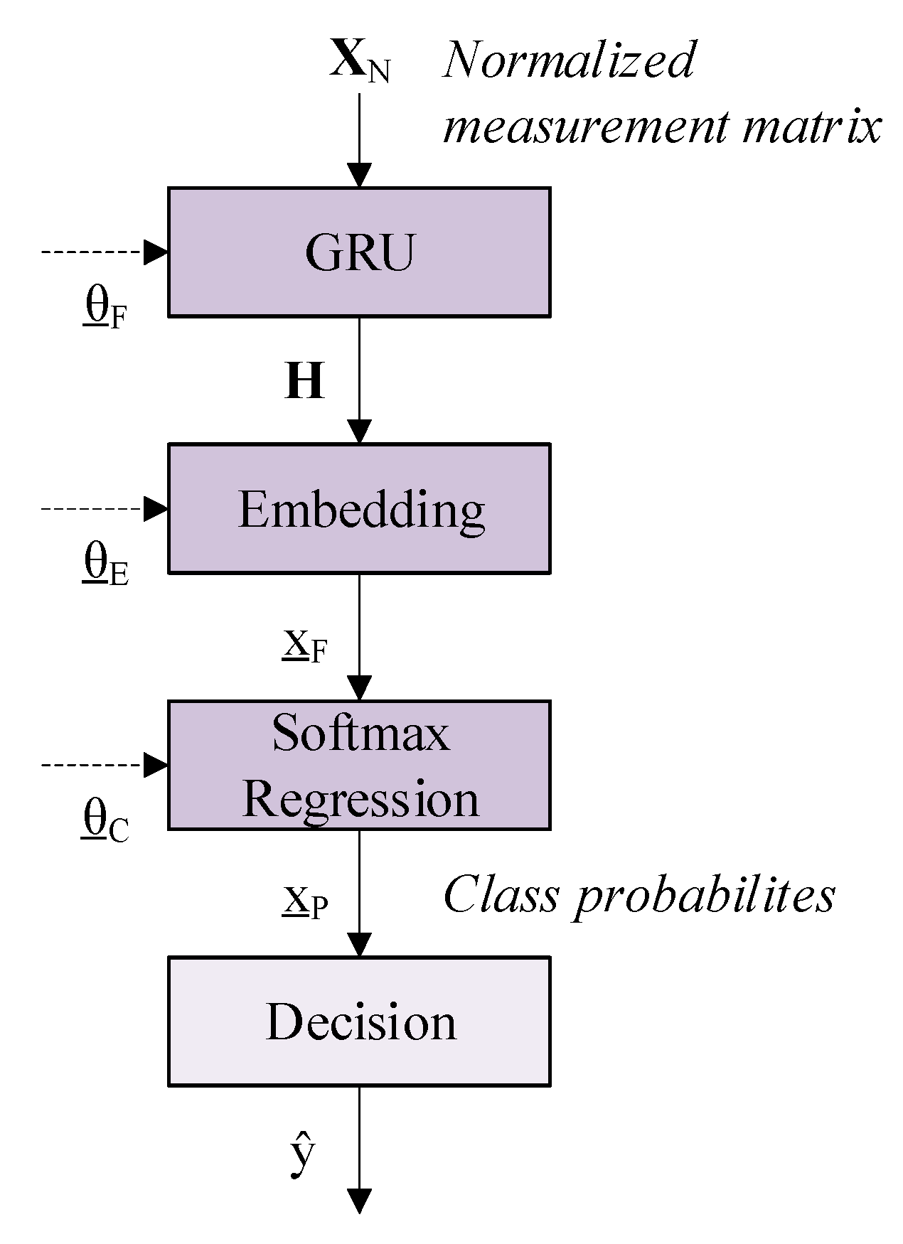
First investigations of a simultaneous disturbance identification and localization were performed in [58] by comparing five different classification approaches. From these results and additional research [59], recurrent neural networks were rated as very suitable for the online classification of grid disturbances regarding the classification accuracy and prediction time. Recurrent neural networks like LSTMs or GRUs can capture autoregressive, non-linear dependencies and time-varying patterns in high-dimensional sequential data by utilizing flexible gating mechanisms within the LSTM or GRU cells. Within this study, GRUs were preferred over LSTMs to increase the robustness and to minimize overfitting problems. The principle workflow of the GRU-based disturbance classification approach is shown in Figure 6.

In the feature extraction step, a hidden state matrix $\mathit{H}$ is computed by a single GRU layer with $Q$ dimensions given the normalized measurement matrix ${\mathit{X}}_{\mathrm{N}}$ and the learned parameters ${\underset{\_}{\theta }}_{\mathrm{F}}$. Afterwards, a feature vector ${\underset{\_}{x}}_{\mathrm{F}}$ of dimension $P$ is generated from the high-dimensional hidden state matrix using an embedding function $f_{\mathrm{E}}$ with ${\underset{\_}{\theta }}_{\mathrm{E}}$. The general equations are given in (9) and (10).

$$\mathit{H}=f_{\mathrm{F}}\left({\mathit{X}}_{\mathrm{N}},{\underset{\_}{\theta }}_{\mathrm{F}}\right)\mathrm{with}\mathit{X}\in {ℝ}^{\mathrm{T}\times \mathrm{K}}\mathrm{and}\mathit{H}\in {ℝ}^{\mathrm{T}\times \mathrm{Q}}$$

(9)

$${\underset{\_}{x}}_{\mathrm{F}}=f_{\mathrm{E}}\left(\mathit{H},{\underset{\_}{\theta }}_{\mathrm{E}}\right)\mathrm{with}{\underset{\_}{x}}_{\mathrm{F}}\in {ℝ}^{\mathrm{P}}$$

(10)

The goal of the embedding function is to capture the necessary information from the hidden state matrix to differentiate between the classes. According to (11) and (12), the classifier $f_{\mathrm{C}}$ is based on a standard softmax regression to compute the class probability vector ${\underset{\_}{x}}_{\mathrm{P}}$ with the parameters ${\underset{\_}{\theta }}_{\mathrm{C}}$ over all $C$ classes.

$${\underset{\_}{x}}_{\mathrm{P}}=f_{\mathrm{C}}\left({\underset{\_}{x}}_{\mathrm{F}},{\underset{\_}{\theta }}_{\mathrm{C}}\right)\mathrm{with}{\underset{\_}{x}}_{\mathrm{P}}\in {ℝ}^{\mathrm{C}}$$

(11)

$${\underset{\_}{x}}_{\mathrm{P}}=\frac{exp\left({\underset{\_}{w}}_C{\underset{\_}{x}}_{\mathrm{F}}+b_C\right)}{{{\displaystyle \sum }}_{C}exp\left({\underset{\_}{w}}_C{\underset{\_}{x}}_{\mathrm{F}}+b_C\right)} \mathrm{with}{\underset{\_}{w}}_C\in {ℝ}^{\mathrm{P}}$$

(12)

The final class assignment $\widehat{y}$ is based on the maximum probability value estimated by the classifier. The parameters of the feature extraction ${\underset{\_}{\theta }}_{\mathrm{F}}$, embedding ${\underset{\_}{\theta }}_{\mathrm{E}}$ and classifier ${\underset{\_}{\theta }}_{\mathrm{C}}$ are learned jointly via backpropagation using the cross-entropy loss formulation given in (13).

$$e=-{\displaystyle \sum }_C{y}_C\log x_{\mathrm{P}}$$

(13)

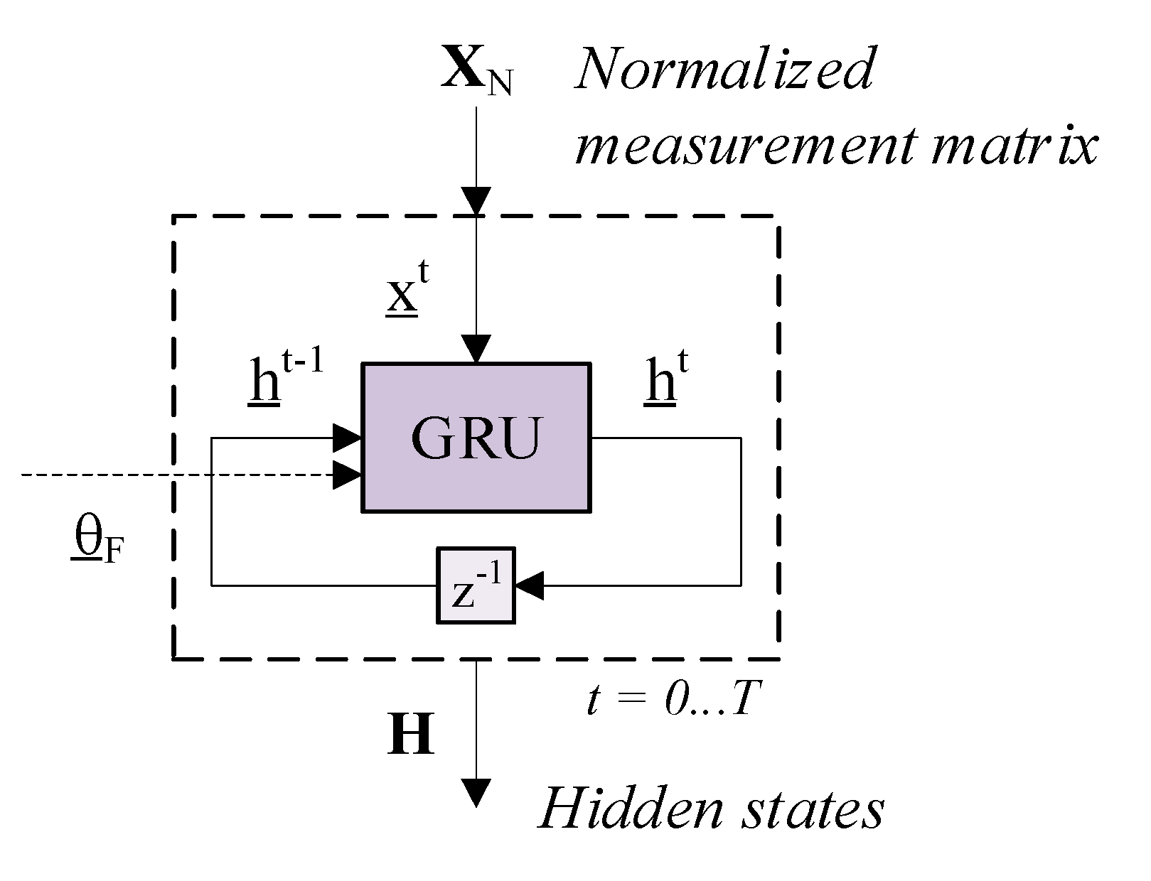
The GRU layer in the feature extraction step contains the most expensive operations in the disturbance classification module. For each time step $t$, the GRU computes a hidden state vector ${\underset{\_}{h}}^t$ using the actual input vector ${\underset{\_}{x}}^t$ and the hidden state vector from the previous time step ${\underset{\_}{h}}^{t-1}$. This is done sequentially over all $T$ time steps to compute the hidden state matrix $\mathit{H}$. The weights and biases of the GRU ${\underset{\_}{\theta }}_{\mathrm{F}}$ are shared among all time steps. The principle workflow is shown in Figure 7.

Inside a GRU, the input vector and the last hidden state vector are used to compute the output vectors of the update gate ${\underset{\_}{z}}^t$ and the reset gate ${\underset{\_}{r}}^t$. From that, a candidate hidden state vector ${\widetilde{\underset{\_}{h}}}^t$ is estimated, which represents the actual information gained by the GRU. In the last step, the new hidden state vector ${\underset{\_}{h}}^t$ is computed depending on the output of the update gate vector, which decides whether to keep the old information (${\underset{\_}{z}}^t\to 1$) or to forget them and to use the new information (${\underset{\_}{z}}^t\to 0$). These gating mechanisms allow a very flexible control over the learned representations and accounts for the vanishing gradient problem when applying backpropagation over time (BPTT). The basic formulations for the gate calculations are given in (14) to (17).

$${\underset{\_}{z}}^t=\sigma \left({\mathit{U}}_{\mathrm{z}}{\underset{\_}{h}}^{t-1}+{\mathit{W}}_{\mathrm{z}}{\underset{\_}{x}}^t+{\underset{\_}{b}}_{\mathrm{z}}\right)\mathrm{with}{\mathit{U}}_{\mathrm{z}}\in {ℝ}^{\mathrm{Q}\times \mathrm{Q}}\mathrm{and}{\mathit{W}}_{\mathrm{z}}\in {ℝ}^{\mathrm{K}\times \mathrm{Q}}$$

(14)

$${\underset{\_}{r}}^t=\sigma \left({\mathit{U}}_{\mathrm{r}}{\underset{\_}{h}}^{t-1}+{\mathit{W}}_{\mathrm{r}}{\underset{\_}{x}}^t+{\underset{\_}{b}}_{\mathrm{r}}\right)\mathrm{with}{\mathit{U}}_{\mathrm{r}}\in {ℝ}^{\mathrm{Q}\times \mathrm{Q}}\mathrm{and}{\mathit{W}}_{\mathrm{r}}\in {ℝ}^{\mathrm{K}\times \mathrm{Q}}$$

(15)

$${\widetilde{\underset{\_}{h}}}^t=\tanh \left({\mathit{U}}_{\mathrm{h}}\left({\underset{\_}{r}}^t\circ {\underset{\_}{h}}^{t-1}\right)+{\mathit{W}}_{\mathrm{h}}{\underset{\_}{x}}^t+{\underset{\_}{b}}_h\right)\mathrm{with}{\mathit{U}}_{\mathrm{h}}\in {ℝ}^{\mathrm{Q}\times \mathrm{Q}}\mathrm{and}{\mathit{W}}_{\mathrm{h}}\in {ℝ}^{\mathrm{K}\times \mathrm{Q}}$$

(16)

$${\underset{\_}{h}}^t={\underset{\_}{z}}^t\circ {\underset{\_}{h}}^{t-1}+\left(1-{\underset{\_}{z}}^t\right)\circ {\widetilde{\underset{\_}{h}}}^t$$

(17)

Despite of the gating mechanisms, the information cannot be maintained over long time periods. As the number of time steps increases, some information might be lost or overwritten such that the final hidden state vector ${\underset{\_}{h}}^{\mathrm{T}}$ does not contain all necessary information to classify the time series. Hence, different embedding functions are proposed to create a representative feature vector from the full hidden state matrix including feedforward neural networks as well as parametric and non-parametric attention models–see Figure 8.

Feedforward neural network-based embedding: A very straightforward solution includes a single layer feedforward neural network with sigmoid activation function applied on the vectorized hidden state matrix. Depending on the number of time steps $T$ and hidden dimensions $Q$, this can result in a large weight matrix ${\mathit{W}}_{\mathrm{S}}$. The equation is given in (18).

$${\underset{\_}{x}}_{\mathrm{F}}=\sigma \left({\mathit{W}}_{\mathrm{S}}vec\left(\mathit{H}\right)+{\underset{\_}{b}}_{\mathrm{S}}\right)\mathrm{with}{\mathit{W}}_{\mathrm{S}}\in {ℝ}^{\mathrm{P}\times \left(\mathrm{T}·\mathrm{Q}\right)}\mathrm{and}{\underset{\_}{b}}_{\mathrm{S}}\in {ℝ}^{\mathrm{P}}$$

(18)

Parametric and non-parametric attention model based embedding: A more efficient approach utilizes attention models to compute a weighted sum of the hidden state vectors–see (19). According to (20), these attention weights ${\alpha }^t$ are computed for each time step using a softmax normalization on the score values $s^t$. In this case, the feature dimension equals the hidden dimension $P=Q$, such that no additional dimension reduction is performed within the embedding function.

$${\alpha }^t=\frac{exp\left(s^t\right)}{{{\displaystyle \sum }}_{t}exp\left(s^t\right)}$$

(19)

$${\underset{\_}{x}}_{\mathrm{F}}={\displaystyle \sum }_t{\alpha }^t·{\underset{\_}{h}}^t$$

(20)

A score value indicates the importance of the current hidden state, such that high score values lead to high attention weights and vice versa. Within the parametric attention model (derived from [60]), a small feedforward neural network with tangent hyperbolic activation function computes the score values–see (21). The network parameters can be shared over time steps (global parametric attention model) or calculated for each time step separately (local parametric attention model).

$$s^t=\tanh \left({\underset{\_}{w}}_{\mathrm{S}}{\underset{\_}{h}}^t+b_{\mathrm{S}}\right)\mathrm{with}{\underset{\_}{w}}_{\mathrm{S}}\in {ℝ}^{\mathrm{Q}}$$

(21)

The non-parametric attention model uses dot-product (22) or cosine similarity (23) to calculate the score values. For this, the actual hidden state ${\underset{\_}{h}}^t$ is compared with the last hidden state ${\underset{\_}{h}}^{\mathrm{T}}$ for each time step.

$$s^t=\langle {\underset{\_}{h}}^t,{\underset{\_}{h}}^{\mathrm{T}}\rangle$$

(22)

$$s^t=\frac{\langle {\underset{\_}{h}}^t,{\underset{\_}{h}}^{\mathrm{T}}\rangle }{\Vert {\underset{\_}{h}}^t\Vert ·\Vert {\underset{\_}{h}}^{\mathrm{T}}\Vert }$$

(23)

3.6. Curative Actions

A main security aspect for the system operation is the maintenance of the N-1 criterion. It is applied to the system operation in such a way, that equipment outages do not result into a violation of operational constraints or limit violations and to prevent cascading outages. The N-1 criterion is conservative in terms of unexploited transmission capacities. “Curative actions are operational measures that are executed immediately after the occurrence of a foreseeable contingency” [61]. Thus, the application of curative actions is suitable to sensitively dissolve or extend the conservative N-1 criterion under certain conditions to gain transmission capacity. It is important to note, that curative actions are selective against distinguished events or critical contingencies. They can include line switching, redispatch or adaptation of VSC active power set points [21].

4. Results from Case Studies

Different datasets are used to evaluate the proposed synchrophasor applications for efficient data processing and post-mortem analysis (see Section 3.2 and Section 3.3) as well as enhanced situational awareness (see Section 3.4 and Section 3.5). These include low- to medium-voltage field measurements as well as high-voltage PMU signals extracted from dynamic grid simulations.

Table 5. Overview of used datasets within this study.

Dataset	# of PMU Stations	Measurement Channels [a]	Voltage Level	Reporting Rate
LVField	5	F, VAMP, VANG, IAMP, IANG, FC	0.4 kV–20 kV	10 f.p.s.
MVField [62]	6	F, VAMP, VANG	0.4 kV–120 kV	30 f.p.s.
HVSim	21	F, VAMP, VANG	400 kV	25 f.p.s.

^[a] F…frequency, V_Amp…voltage amplitude, V_Ang…voltage angle, I_AMP…current amplitude, I_ANG…current angle, FC…rate of change of frequency.

gives a short overview.

The LVField dataset contains synchrophasor measurements of five PMUs from a public vendor, which are placed at a low-voltage distribution grid in Germany. The M-class PMUs provide three-phase voltage and current phasors (12 phasors per PMU) as well as frequency and rate of change of frequency values at 10 f.p.s reporting rate. The total record time covers 16.5 h. The MVField dataset contains measurements from the Texas Synchrophasor Network. It contains a 1 h record of single-phase voltage phasors and frequency measurements from six different PMUs placed at a medium-voltage distribution grid. Further information as well as the dataset provides [62]. In contrast to the previous datasets, the HVSim records are based on dynamic grid simulations from a generic transmission power grid. The synthetic PMU signals comprise of single-phase voltage phasors and frequencies from 21 PMUs (25 f.p.s. reporting rate). Detailed descriptions are given in the following Section 4.1.

4.1. Dynamic Grid Simulations

4.1.1. Grid Topology and Key Assumptions

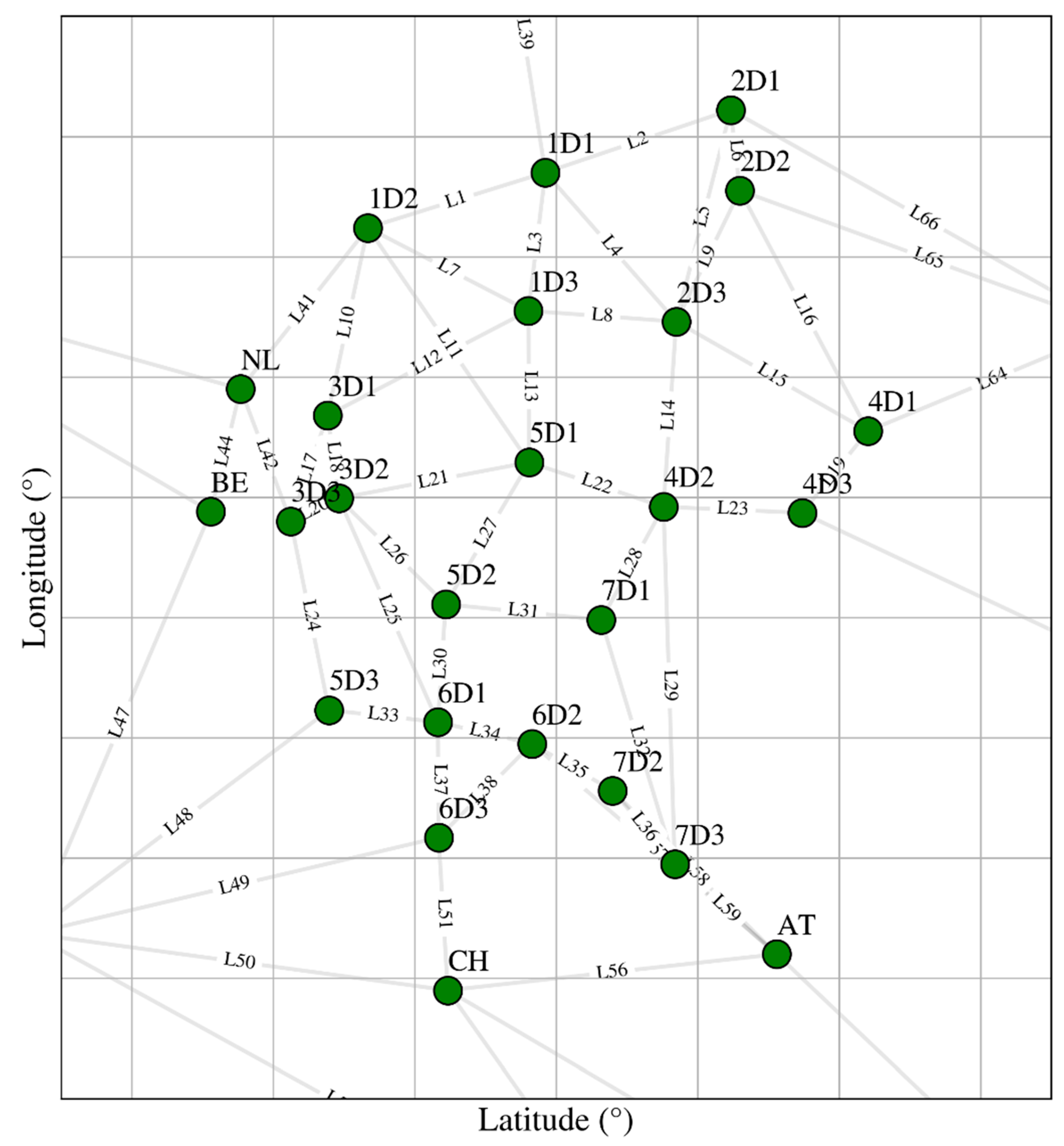
For the HVSim dataset, a single-phase grid model based on the ENTSO-E European Transmission System is used to facilitate the modelling and the analysis of the dynamic behavior of the power system. The 380 kV transmission system consist of 33 substations, where each interconnection consists of multiple circuit transmission lines to ensure the N-1 criteria. In order to emulate the dynamic of the system under outage conditions or load/generation changes, some generator units are equipped with Automatic Voltage Regulators (AVR) and Power System Stabilizers (PSS) to ensure the system stability in the simulated scenarios. Furthermore, multiple protection mechanisms for generators and lines are modeled. The frequency protection maintains the generator connected for frequency ranges between 47.5 Hz to 51.5 Hz and disconnects them otherwise for 5 s to 30 s to preserve the technical integrity of the equipment. Additionally, a fault-ride-through (FRT) capability for the generators protects the equipment under long duration short circuits. Finally, a simple maximum loading protection schema is implemented for the lines, which allows a line overloading for short time periods (<5 s). The implementation of these protection scheme allows simulating cascading effects for certain grid states. The basic grid topology with station and line labels is given in Figure 9. In a preprocessing step, different generation and load conditions are evaluated using optimal power flow (OPF) simulations. For a selected number of suitable steady states or operational points, different contingencies are simulated using RMS symmetric simulations with 1 ms time steps. A DIgSILENT^® Programming Language (DPL) script controls the simulations with regard to events creation, stability check and saving of the results. For each operational point, about 440 different contingencies are simulated considering generator outages, line trips, short circuits at different line positions, partial photovoltaic (PV) outages as well as partial load losses. An online assessment of the simulated signals checks the system stability and aborts the current simulation in case of violations of predefined frequency or voltage limits. The RMS values are averaged to extract PMU signals at the given temporal resolution of 40 ms (corresponds to 25 f.p.s.). Compared to field measurements, the phasor estimation procedure and consequent signal deviations (e.g., filtering effects) are neglected.

4.1.2. Dynamic Simulation Results

For a better illustration of the dynamic grid model, some exemplary contingencies are presented for simulated frequency and voltage magnitude signals from four different PMUs. Figure 10 shows the corresponding simulations results over a period of 10 s for a partial PV plant outage of 50% installed capacity for two different operational points. In both cases, a frequency drop of about 20 mHz can be noticed resulting from a 0.5 MW PV capacity loss (about 1 MW nominal capacity). The voltage magnitudes increase from steady conditions of up to 1.5 kV in adjacent substations. A comparison between both operational points reveals minor differences between frequency signals but larger deviations between voltage magnitude signals due to the difference in the supplied reactive power. A short circuit at 90% length of line L19 is shown in Figure 11 for the same PMU sensor signals and operational points. Compared to the previous contingency, the frequency is oscillating within the first seconds of the disturbance between +20/−40 mHz and returns slowly to the pre-disturbance frequency level of 50 Hz. Characteristic voltage drops of about 110 kV can be observed for both operational points shortly after the disturbance event.

4.2. Validation of Synchrophasor Applications Using Field Measurements

4.2.1. Results from Spatiotemporal Synchrophasor Data Compression

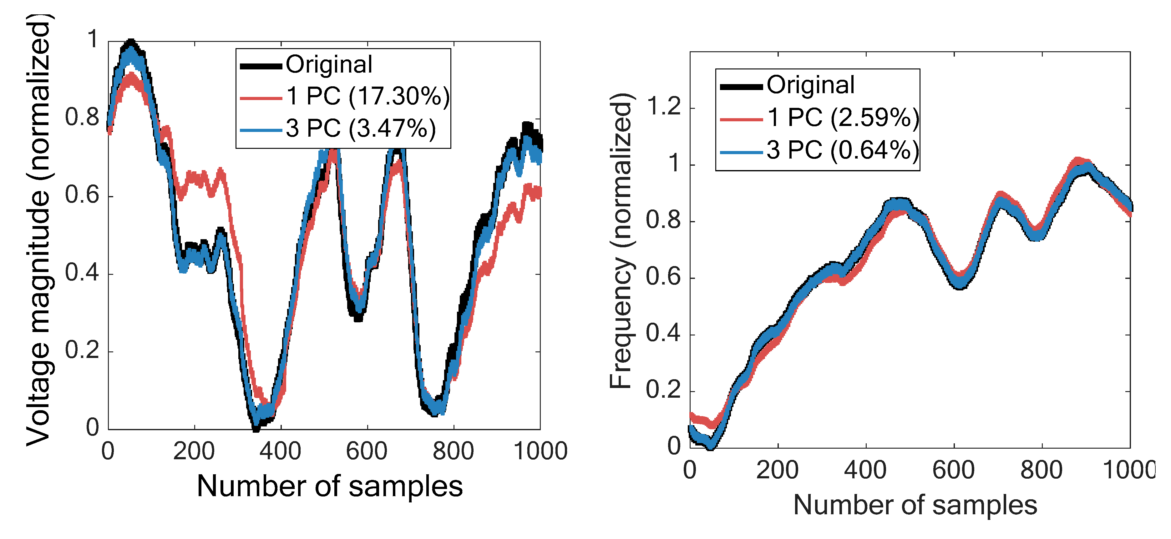
The evaluation of the spatiotemporal data compression module is based on the LVField dataset. The spatiotemporal compression algorithm is applied on randomly selected measurement records with a fixed time range of 100 s (1000 observations). Within the data pre-processing, the raw measurement values are normalized into the range [0,1] and filtered using backward sliding moving averages to eliminate high-frequency oscillations. To avoid signal discontinuities, the voltage and current phase angles are unwrapped before normalization. Regarding Section 3.2, the evaluation is focused on PCA as spatial and DWT as temporal compression algorithm whereas the chosen DWT hyperparameters are given in

Table 6. Hyperparameters of the spatiotemporal synchrophasor data compression module.

Hyperparameter	Value
Wavelet function	Db5
Decomposition level	2
Coefficient threshold	0.05

. The number of principle components is varied during the evaluation. Original and reconstructed voltage magnitude and frequency values are compared in Figure 12 for one and three principle components. Increasing the number of principle components reduces the compression rate roughly from 17 to 5. At the same time, the reconstruction error raises from 3.47 to 17.30 for voltage magnitudes and from 0.64 to 2.59 for frequencies. As a result, high deviations between original and reconstructed signals can be observed when reducing the number of principle components.

Spatial, temporal and total compression rates $r_C$ as well as reconstruction errors $e_R$ are summarized for the different measurement channels in

Table 7. Compression rates and reconstruction errors for different measurement channels.

Channel	Spatial		Temporal		Total
	${\mathit{r}}_{\mathit{C}}$	${\mathit{e}}_{\mathit{r}}$	${\mathit{r}}_{\mathit{C}}$	${\mathit{e}}_{\mathit{r}}$	${\mathit{r}}_{\mathit{C}}$	${\mathit{e}}_{\mathit{r}}$
Voltage (magnitude)	1.656	0.035	3.571	0.008	5.814	0.036
Voltage (angle)		0.001		0.001		0.001
Current (magnitude)		0.034		0.006		0.035
Current (angle)		0.001		0.004		0.003
Frequency		0.006		0.008		0.010
ROCOF		0.058		0.016		0.060

assuming three principle components used within the spatial compression stage.

Using three principle components reduces the compression rate up to 5.8 and the reconstruction error up to 0.04. The highest reconstruction errors can be observed especially during the spatial compression and for voltage magnitude signals. The reconstruction errors heavily depend on the signal variability and the deviations within the different measurement channels. Assuming 1000 observations, a single measurement record of one voltage and current phasor as well as one frequency and ROCOF signal comprises 240 kByte memory space allocation. Specific file formats or additional over-head information are not considered here. The size of the compressed dataset varies between 14 kByte and 40 kByte depending on the number of principle components used in the spatial compression stage. The necessary calculations are performed in Matlab^® with the implementation of an additional toolbox for wavelet decomposition [63].

4.2.2. Results from Synchrophasor Disturbance Extraction

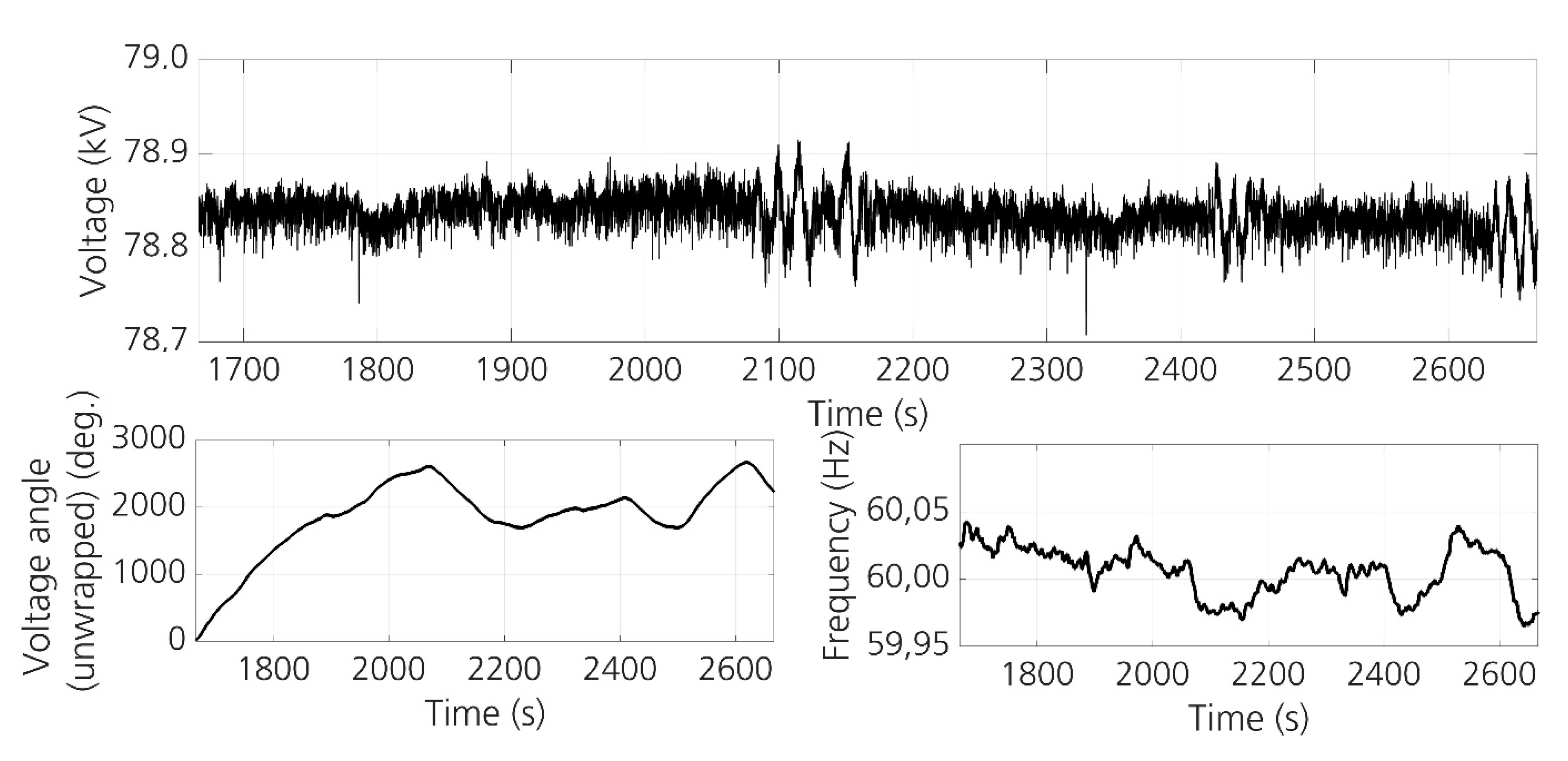
The evaluation of the disturbance extraction module is based on the MVField dataset including voltage magnitudes and angles as well as frequencies from different PMU sensors at medium-voltage level. The reporting rate is 30 f.p.s. Before preprocessing, high frequency components are eliminated from the raw measurements using a wavelet based denoising. A chosen time section of about 15 min of the raw voltage phasors and frequencies is given in Figure 13.

From visual inspection, some disturbances can be noticed including voltage oscillations at 2100 s, 2450 s and 2650 s as well as voltage sags at 1650 s, 1800 s and 2340 s. Additionally, the voltage oscillations seem to coincide with frequency drops of about 50 mHz and 70 mHz. It can be expected that these events are captured from the disturbance extraction module automatically. The chosen hyperparameters of the different submodules are listed in

Table 8. Hyperparameters used for the disturbance extraction module.

Hyperparameter	Value
S transform max. frequency	1 Hz
DWT decomposition level	12
DWT wavelet function	Db5
Isomap number of nearest neighbors	50
SiLiOd distance function	Mahalanobis
LOF & COP distance function	Euclidean
LOF & COP number of nearest neighbors	50

. The influence of changing hyperparameters is investigated in [49].

The disturbance extraction module is applied on a historical record of a single measurement channel. Within this survey, results are shown for the voltage magnitude measurements. The dataset is sampled with a window length of 3000 time steps (100 s) and normalized into the range [0,1]. The definition of the window length is crucial for the disturbance extraction module and should be selected in accordance with the expected disturbance time spans.

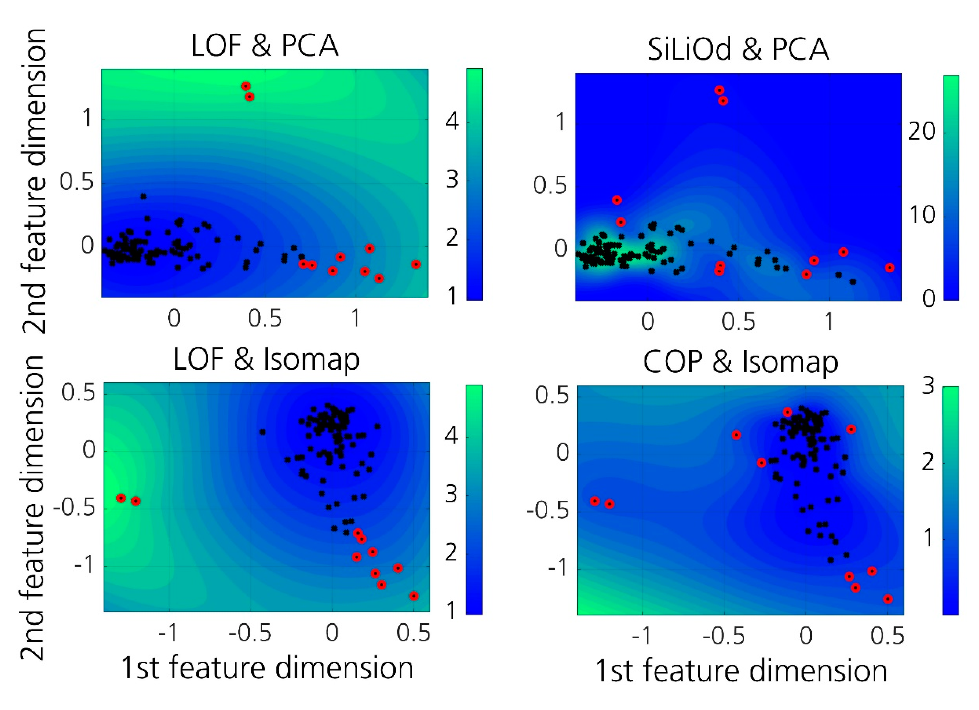
The outlier detection algorithms compute outlier scores for all samples depending on their deviation from the major signal behavior. Figure 14 shows the distribution of outlier scores (outlier map) for different combinations of outlier detection and dimension reduction techniques using time domain features. The 10 samples with highest outlier scores (top-10 outliers) are additionally highlighted in red.

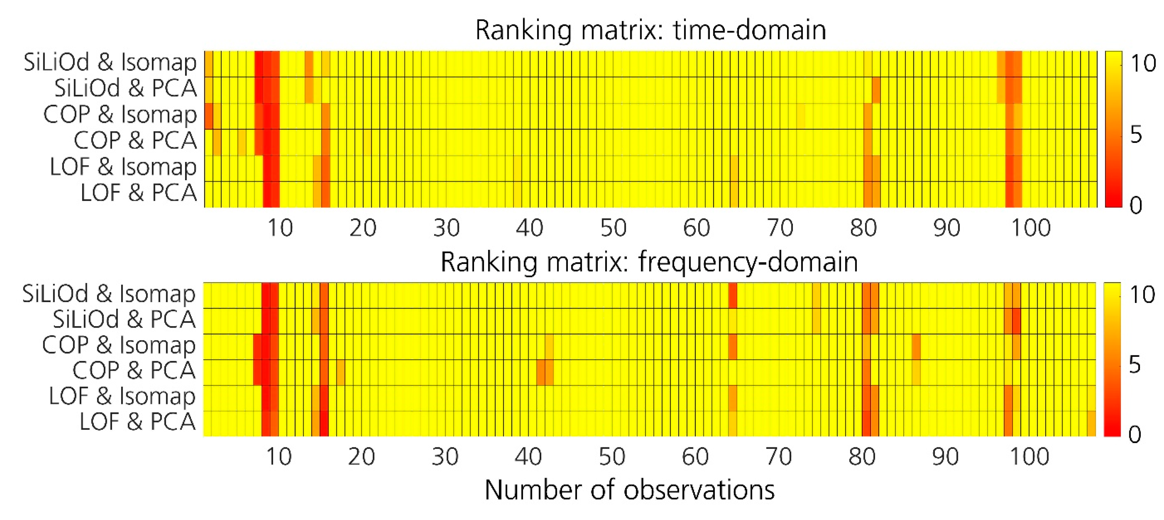
The majority of data points are clustered close together and correspond to samples with very similar features and signal behavior. For the LOF and COP, the outlier score decreases for data points with a high distance to the center, while SiLiOd shows opposite behavior due to the different metric calculation (see also Section 3.3). Additionally, PCA and Isomap compute slightly different feature embeddings, which increases the variance of the results of the different base detectors. In all cases, LOF, COP and SiLiOd mainly agree when detecting far-away outliers (data points with high distance to center), but disagree when detecting near-by outliers (data points with medium or low distance to center). Due to their low distances to neighboring data points, near-by outliers are more difficult to detect and to distinguish from the majority signal behavior. As stated in Section 3.3, the outlier scores of the different base detectors are aggregated via rank transformation and passed to the clustering stage. For a better illustration, Figure 15 shows the rank transformed top-10 outliers for all base detectors in the time and frequency domain. Low outlier ranks correspond to high outlier scores and vice versa. A high agreement among all base detectors and domains can be observed for the samples 8, 9, 97 and 98 indicating a high outlier degree and a potential disturbance. These samples are assigned with low total rank values. Other samples like 43, 65 or 85 are only detected by a minority of the base detectors which results in a lower certainty of the results and higher total rank values. Figure 16 gives some exemplary results for disturbed patterns (low total ranks) and undisturbed patterns (high total ranks). In case of the disturbed signal patterns, sample 6 corresponds to a voltage sag and sample 10 corresponds to a voltage oscillation. From Figure 15, sample 10 with the voltage oscillation shows low total ranks among all base detectors in the time- and frequency-domain. In contrast to that, sample 6 with the voltage sag can only be detected by a few base detectors in the time-domain resulting in high total ranks. This maybe a result of the short time span of the disturbance compared to the window size.

The necessary calculations are performed in Matlab^® with an additional open-source implementation for the S transform [63,64] and a JAVA^® based library for Isometric mapping [65]. The outlier detection methods were taken from the JAVA^® based ELKI (Environment for Developing KDD-Applications Supported by Index-Structures) data mining framework [66].

4.3. Validation of Synchrophasor Applications Using Dynamic Grid Simulations

4.3.1. Results from Synchrophasor Disturbance Detection

The disturbance detection module is evaluated for different contingencies using dynamic grid simulations from the HVSim dataset as described in Section 4.1. A fixed hyperparameter set has been chosen according to

Table 9. Hyperparameters used for the disturbance detection module.

Hyperparameter	Value
S transform max. frequency	10 Hz
# of S transform frequency bins	50
# of samples for feature assessment N	20
# of time steps per sample	50

.

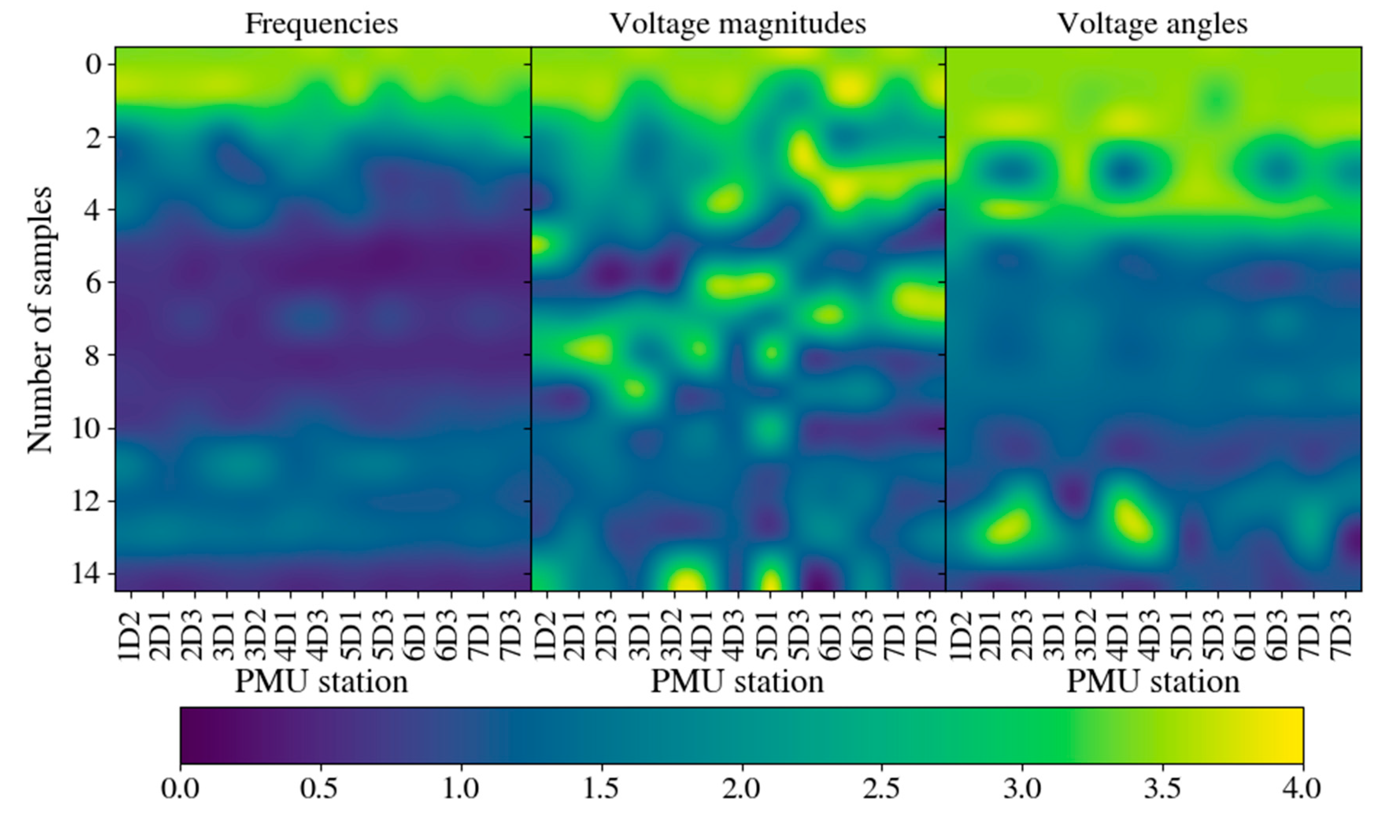
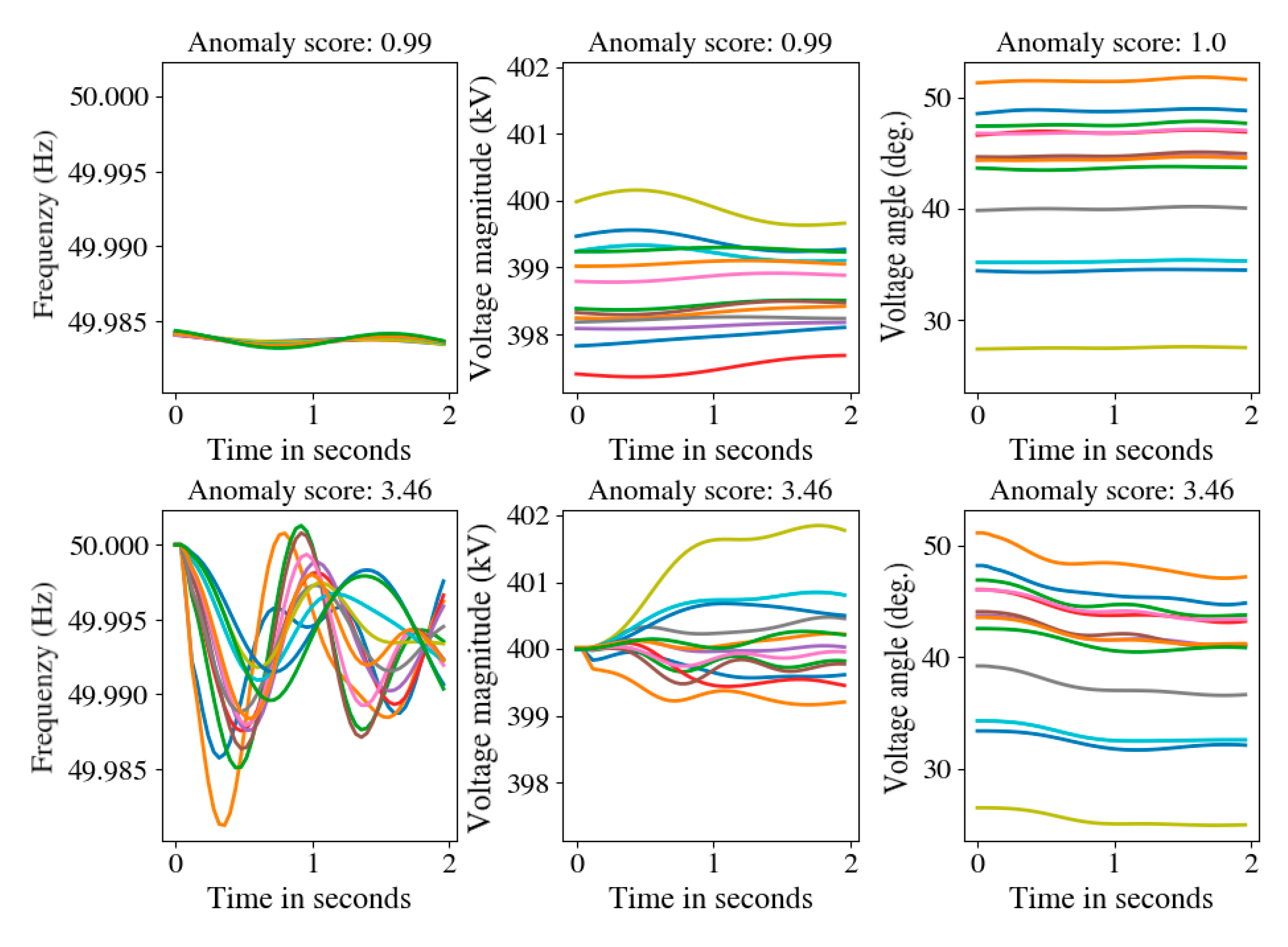
The disturbance detection module is applied to assess features from 13 different PMU stations. For each PMU measurement channel, the last 50 observations (corresponds to 2 s) are used to generate the features in time and frequency domain. The resulting feature vector is compared with the features from the last N samples to compute the anomaly scores (see also Section 3.4). Some exemplary results are shown in Figure 17 and Figure 18 for two different contingencies. It can be seen that high anomaly scores occur mainly within the first PMU samples, which represents the beginning of a disturbance and usually causes high signal variations and fluctuations. During this time period, there is a transition from steady to transient system states. For subsequent PMU samples, the anomaly scores decrease depending on the measurement and the disturbance type. Especially in case of the line outage, high anomaly scores can be observed for voltage magnitudes over the whole timespan, while the frequency values almost remain unchanged. For a better understanding, some exemplary signal patterns of low and high anomaly scores are given in Figure 19. Each frequency, voltage magnitude or voltage angle signal represents a single PMU station.

Clear differences can be observed between patterns with low and high anomaly score. At low anomaly scores below or equal 1.0, only small signal variations occur over time for frequency, voltage magnitude and voltage angle signals. At high anomaly scores between 3.0 and 4.0, high frequency oscillations are present as well as significant changes of voltage magnitude and angle signals over time. The necessary calculations are performed in Python^® with additional packages for wavelet decomposition [67] and statistical analysis [68].

4.3.2. Results from Synchrophasor Disturbance Classification

For the evaluation of the disturbance classification module, dynamic grid simulations are used as described in Section 4.1. The base scenario comprises 20 different contingencies or disturbance classes, which are concentrated at 4 different stations and lines in the grid–as shown in

Table 10. Class configuration containing disturbance locations and types.

Location	Type	Label
Station 1D1	Outage of DKW generator	1D1.DKW_OT
Station 2D3	Outage of GKW generator	2D3.GKW_OT
Station 4D2	Outage of GKW generator	4D2.GKW_OT
Station 6D1	Outage of DKW generator	6D1.DKW_OT
Station 1D1	PV partial outage of 25%	1D1.PV_LC_25
Station 2D3	PV partial outage of 50%	2D3.PV_LC_50
Station 4D2	PV partial outage of 75%	4D2.PV_LC_75
Station 6D1	PV partial outage of 50%	6D1.PV_LC_50
Station 1D1	Load loss of 75%	1D1.L1_LC_75
Station 2D3	Load loss of 50%	2D3.L1_LC_50
Station 4D2	Load loss of 25%	4D2.L1_LC_25
Station 6D1	Load loss of 50%	6D1.L1_LC_50
Line 7	Line trip	L7_OT
Line 19	Line trip	L19_OT
Line 24	Line trip	L24_OT
Line 32	Line trip	L32_OT
Line 7	Short circuit at 10% line length	L7_SC_10
Line 19	Short circuit at 90% line length	L19_SC_90
Line 24	Short circuit at 50% line length	L24_SC_50
Line 32	Short circuit at 10% line length	L32_SC_10

. Generator outages are distinguished between small power plants (DKW) and large power plants (GKW). PV power plant outages and load losses are modelled as partial outages related to their installed capacities. Short circuits are modelled as 3-phase line-to-ground faults with varying fault location with regard to the line length. These disturbances are simulated for three operational points with different generation (renewable and conventional) and load profiles. The main parameters of the base scenario are given in

Table 11. Parameters of the base scenario.

Scenario Parameter	Value
Measurement channels	Voltage magnitudes Frequencies
# of PMUs	13
PMU reporting rate	25 f.p.s.
Time window	2 s
Post-disturbance time	10 s
# of operational points	3
Sample overlapping (training) (%)	50
Sample overlapping (validation) (%)	50
Sample overlapping (test) (%)	90
# of samples (training)	540
# of samples (validation)	108
# of samples (test)	3060

concerning the used input data, the time windows and the number of instances in training, validation and test phase. The time window equals the sampling window $T$, while the post-disturbance time corresponds to the total time range for a disturbance event. Training, validation, and test instances contain the same disturbance classes and operational points but differ with respect to the number of samples included into the datasets which depends on the degree of overlapping between subsequent samples. The following results relate to the base scenario and a GRU-based classifier with a local parametric attention model (compare with Section 3.5).

Table 12. Hyperparameters used for the disturbance classification module.

Hyperparameter	Value
# of hidden dimensions $Q$	15
# of feature dimensions $P$	15
Optimizer	rmsprop [69]
Learning rate	0.01
Batch size	50
Maximum # of epochs	1000

summarizes the chosen hyperparameters for the model. Hidden and feature dimensions are equal due to the attention based embedding function. Optimizer, learning rate and batch size are chosen by extensive investigations with different hyperparameter settings.

Additionally, early stopping was used to limit the number of training epochs and prevent overfitting.

Table 13. Accuracies and F1-scores for training, validation and test predictions.

Metric	Training	Validation	Test
Accuracy (%)	97.92	89.81	94.80
F1-score (macro) (%)	97.91	89.01	94.73
F1-score (micro) (%)	97.92	89.81	94.80

shows the accuracy and F1-score results of the training, validation and test datasets for a single training run. Appendix A gives additional information for calculating both metrics.

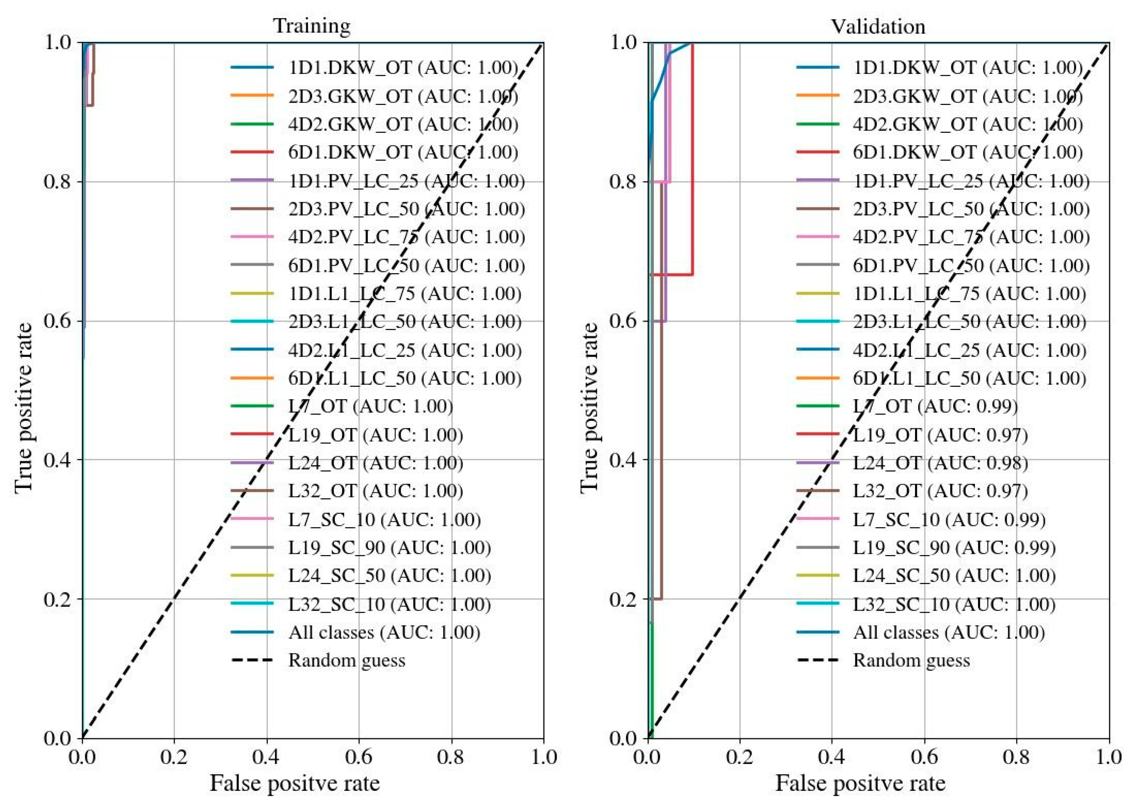
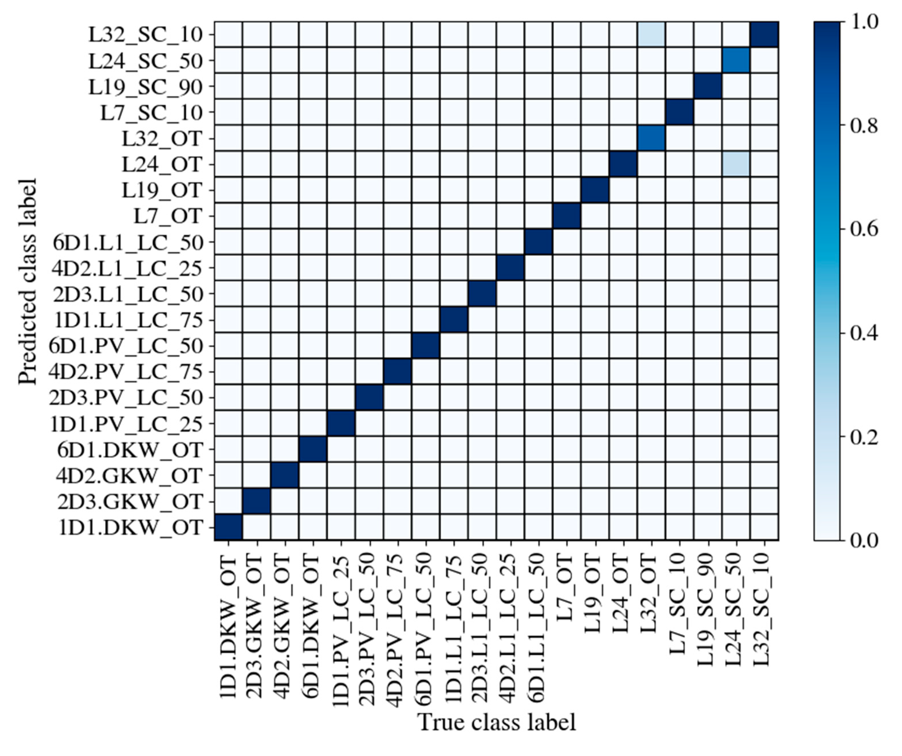
The validation accuracy and F1-score are quite low compared to the training and validation test due to the small size of the validation dataset. The test performance is between the training and the validation values as a result of the high number of samples. Additionally, the training and validation instances cannot be excluded from the test dataset, because of the different sampling rates. Figure 20 shows the normalized confusion matrix for the true and predicted class labels from the training dataset. Very high accuracies can be observed for the conventional and renewable power plant outages as well as the load losses. A few misclassified training instances occur for line trips and short circuits of Line 32. Also in other cases, it can be seen that a correct differentiation between line trips and short circuits represents a big challenge for the PMU based disturbance classification task. One possible reason could be the short duration of these events, which makes a classification difficult for samples with a large time lag to the start of the disturbance. Similar conclusions arise from the receiver operating characteristic (ROC) analysis of the training and validation predictions shown in Figure 21. In accordance with the previous findings, accuracy drops between training and validation can be observed for line outages (minimum AUC value: 0.97) and short circuits (minimum AUC value: 0.99). Other disturbance classes are affected only marginal.

In further investigations, the embedding functions are compared with each other for different numbers of hidden dimensions, learning rates and optimizers. The training, validation and test performance results are given in Figure 22. Highest accuracies can be achieved in case of the local parametric attention model (“local scoring”) with 95.12% (training) and 90.89% (test) as well as the non-parametric attention model using cosine similarity (“cosine attention”) with 94.58% (training) and 91.96% (test). In case of no embedding with 90.54% (training) and 86.53% (test), the last hidden state ${\underset{\_}{h}}^T$ is used as the feature vector. In general, attention based embedding functions increase the test accuracy about 4–5%. Feedforward neural network based embedding functions show very low accuracies on the training (max. 85.88%), validation (max. 78.94%) and test datasets (max. 79.89%) and even perform worse than the “no embedding” variant. This could be due to the vectorization of the hidden state matrix ignoring the dependencies between the hidden state vectors. In contrast to that, attention-based embeddings are more effective to summarize the information across the time steps but keep the number of hidden dimensions unchanged. This can lead to performance degradations when calculating distances between the high-dimensional feature vectors.

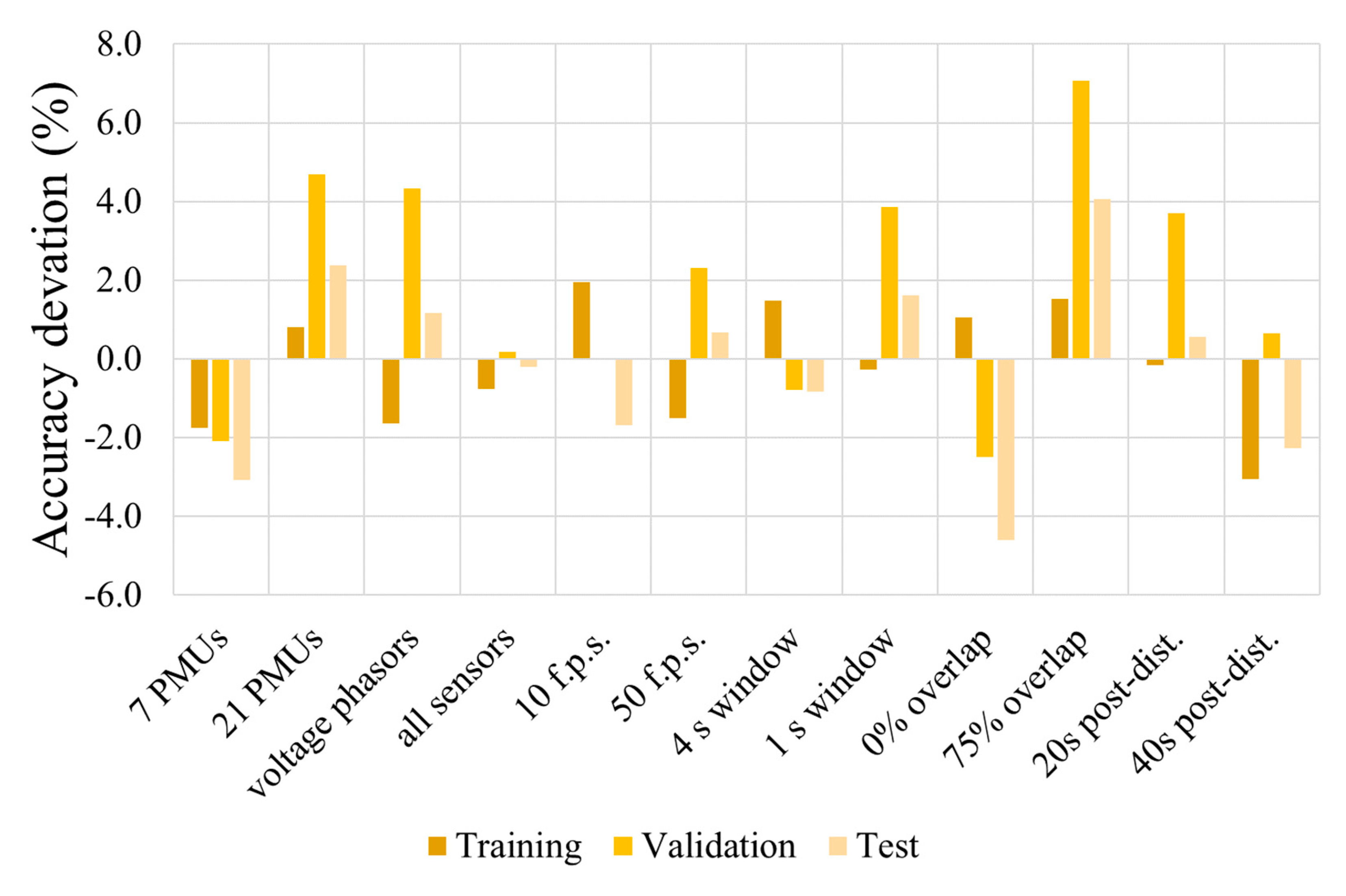
Furthermore, some parameters of the base scenario are varied to evaluate their influence on the classification accuracies. For this, a GRU-based classifier with a local parametric attention based embedding function is investigated using different hidden dimensions. The average accuracy deviations to the base scenario are shown in Figure 23. Larger changes in the test accuracies can be observed when decreasing (−3.1%) or increasing (+2.4%) the number of available PMUs, decreasing (−4.5%) or increasing (+4.1%) the sample overlapping of the training instances and increasing the post-disturbance time from 10 s to 40 s (−2.3%). A higher number of PMUs or sample overlapping increases the input data size and improves the classification accuracies. In contrast to that, a high post-disturbance time complicates the recognition of disturbances especially with short disturbance durations like short circuits or line outages. The sole use of voltage magnitudes and angles as input measurements reduces the training accuracy (−1.6%) but increases the test accuracy (+1.1%). Combining voltage phasors and frequencies has no significant impact on the test accuracy (−0.2%). The necessary calculations are performed in Python^® with additional packages for statistical analysis [68] as well as for creating and training of neural networks [70].

5. Synchrophasor Online Visualization Tool for Enhanced Operator Guidance

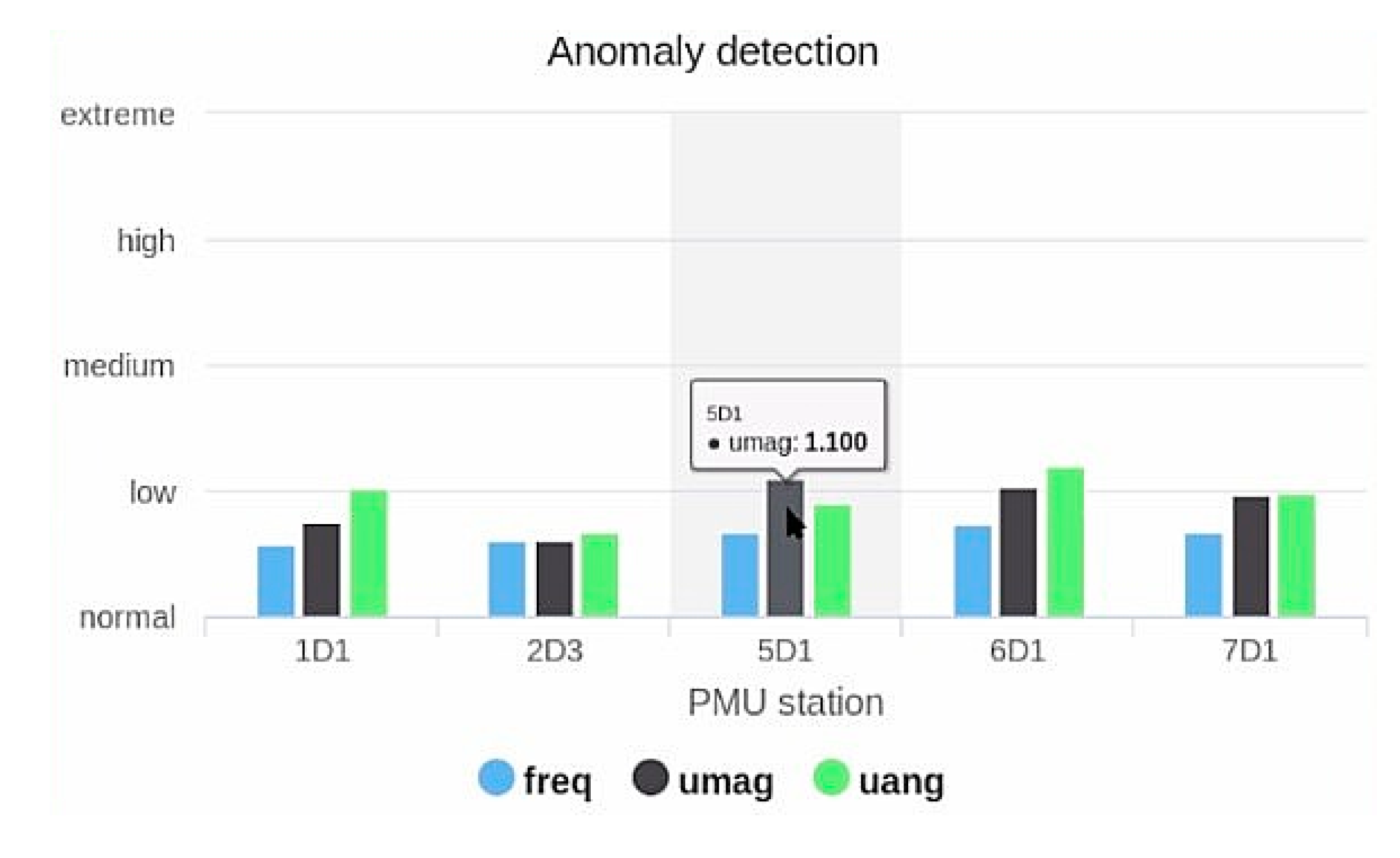
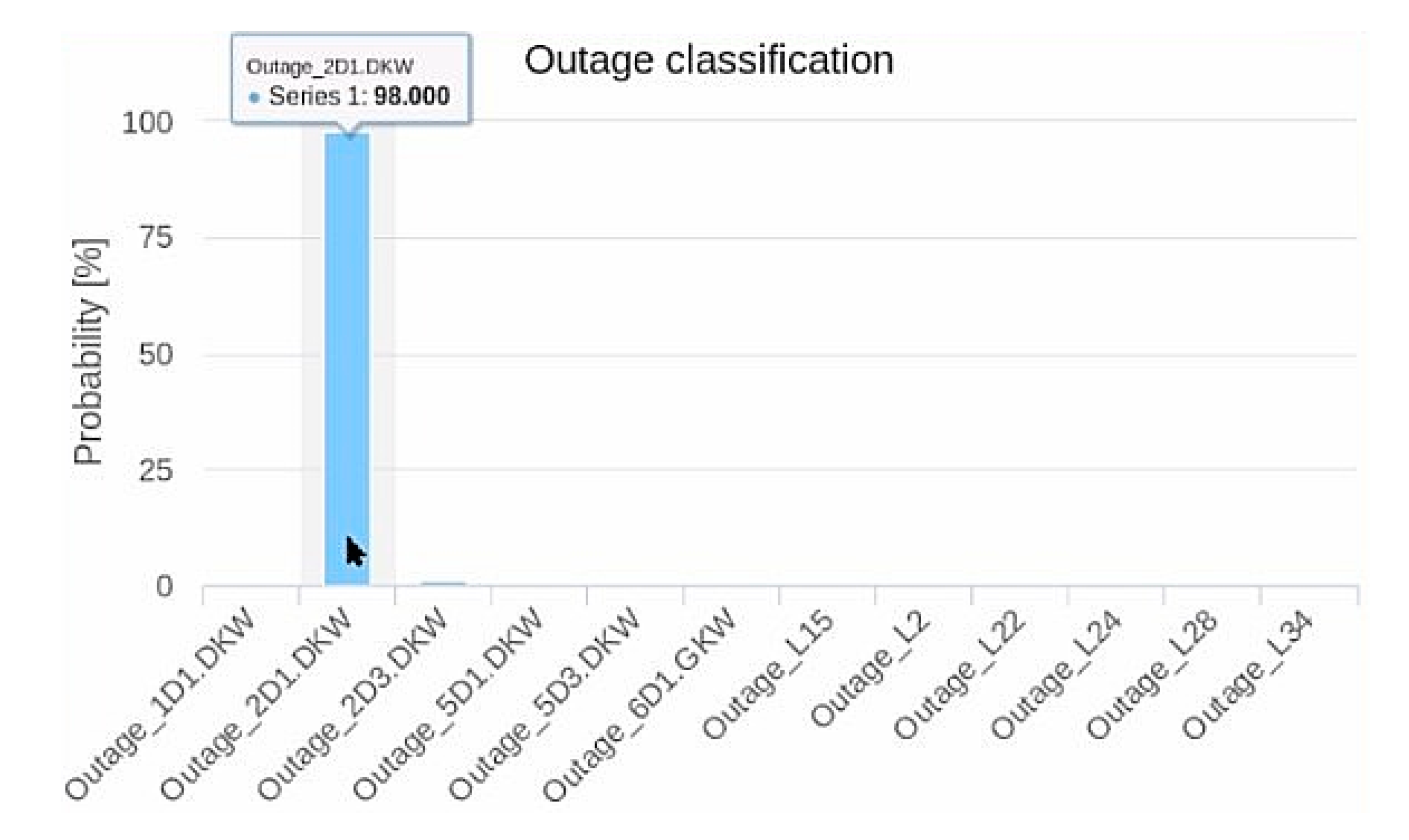
For a better integration into existing control center architectures, a web-based online visualization tool has been developed for the proposed synchrophasor application modules. The application results are written into a PostgreSQL^® database and continuously updated at the front end applying the Highcharts^® visualization framework. This enables a good interpretability of the results and gives the operator access to the online PMU streaming data as well as notifications for potential disturbances or critical system states. Some exemplary visualization charts for the disturbance detection module and disturbance classification module are given in Figure 24.

6. Conclusions and Future Work

In this study, a novel framework is presented with additional visualization capabilities for efficient processing and analyzing historical as well as online PMU data streams. Integrated into existing control centers, this framework provides valuable information for the automated online detection and classification of critical system states as well as the activation of suitable countermeasures to maintain secure system operation. The framework comprises of different application modules for efficient data processing (spatiotemporal data compression module), post-mortem analysis (disturbance extraction module) and online recognition (disturbance detection and classification module). Compared to existing approaches, this framework enables a comprehensive situational awareness to recognize known disturbance events, which belong to simulated contingencies, or new disturbance events, which are revealed post-mortem from efficient analysis of large historical measurements. Within different case studies incorporating field measurements at distribution level as well as dynamic grid simulation data at the transmission level, the proposed application modules are evaluated. The investigations comprise of different recognition tasks including the spatio-temporal compression of measured PMU signals with an average compression rate of 5.8, the detection and extraction of different voltage sag and oscillation events from historical PMU voltage signals as new disturbance events, the computation of anomaly scores for abnormal PMU signals as well as the automated identification and localization of predefined contingencies (e.g., short circuits at different line positions, generator and line trips, partial PV and load losses). High accuracies of about 95% can be achieved with a GRU based classification model and an attention based embedding function. Additionally, a web-based visualization is presented to integrate analysis results into subsequent decision processes for system operation. Future work would comprise the demonstration of a combined disturbance classification and automated selection of curative actions for critical system events. An evaluation of defined benchmark grids is preferable for a better comparison with similar research. Additionally, cyber-security issues should be taken into account in order to increase the robustness of the application modules in case of data manipulations or communication interruptions. A combined online compression and encryption of PMU data streams could be a promising solution for secure and effective data transmission.

References

1. Tielens, P.; van Hertem, D. The relevance of inertia in power systems. Renew. Sustain. Energy Rev. 2016, 55, 999–1009. [Google Scholar] [CrossRef]
2. Rezkalla, M.; Pertl, M.; Marinelli, M. Electric power system inertia: Requirements, challenges and solutions. Electr. Eng. 2018, 100, 2677–2693. [Google Scholar] [CrossRef] [Green Version]
3. Grossman, P.Z.; Cole, D.H. (Eds.) The End of A Natural Monopoly: Deregulation and Competition in the Electric Power Industry; Routledge: London, UK, 2014. [Google Scholar]
4. Brahma, S.; Kavasseri, R.; Cao, H.; Chaudhuri, N.R.; Alexopoulos, T.; Cui, Y. Real-Time Identification of Dynamic Events in Power Systems Using PMU Data, and Potential Applications—Models, Promises, and Challenges. IEEE Trans. Power Deliv. 2017, 32, 294–301. [Google Scholar] [CrossRef]
5. Sass, F.; Sennewald, T.; Brosinsky, C.; Westermann, D.; Mangold, M.; Heyde, C.; Becher, S.; Krebs, R. Control Center Implementation of Advanced Optimization and Decision Support Applications. In Proceedings of the 2018 International Conference on Smart Energy Systems and Technologies (SEST), Sevilla, Spain, 13–14 November 2018; pp. 1–6. [Google Scholar]
6. Liu, Y.; Wu, L.; Li, J. D-PMU based applications for emerging active distribution systems: A review. Electr. Power Syst. Res. 2020, 179, 106063. [Google Scholar] [CrossRef]
7. Dahal, N.; Abuomar, O.; King, R.; Madani, V. Event stream processing for improved situational awareness in the smart grid. Expert Syst. Appl. 2015, 42, 6853–6863. [Google Scholar] [CrossRef]
8. IEEE Standard for SCADA and Automation Systems; C37.1-2007; IEEE: Piscataway, NJ, USA, 2008.
9. Maghsoodlou, F.; Masiello, R.; Ray, T. Energy management systems. IEEE Power Energy Mag. 2004, 2, 49–57. [Google Scholar] [CrossRef]
10. Nuthalapati, S. Power System Grid Operation Using Synchrophasor Technology; Springer International Publishing: Cham, Switzerland, 2019. [Google Scholar]
11. Fernwirkeinrichtungen und -systeme—Teil 5-104: Übertragungsprotokolle—Fernwirkeinrichtungen und -systeme —Teil 5-104: Übertragungsprotokolle—Zugriff für IEC 60870-5-101 auf Netze mit genormten Transportprofilen. DIN EN 60870-5-104:2006 (IEC 60870-5-104:2006). Available online: https://webstore.iec.ch/publication/3746 (accessed on 10 September 2018).
12. IEEE Standard for Electric Power Systems Communications-Distributed Network Protocol (DNP3); IEEE: Piscataway, NJ, USA, 2012; pp. 1815–2012.
13. Morisson, K.; Kamwa, I.; Glavic, M. Review of On-Line Dynamic Security Assessment Tools and Techniques: Cigré WG C4.601; Technical Brochure No. 325; CIGRE: Paris, France, 2007. [Google Scholar]
14. Phadke, A.G.; Pickett, B.; Adamiak, M.; Begovic, M.; Benmouyal, G.; Burnett, R.O.; Cease, T.W.; Goossens, J.; Hansen, D.J.; Kezunovic, M.; et al. Synchronized sampling and phasor measurements for relaying and control. IEEE Trans. Power Deliv. 1994, 9, 442–452. [Google Scholar] [CrossRef]
15. IEEE/IEC International Standard—Measuring Relays and Protection Equipment—Part 118–1: Synchrophasor for Power Systems—Measurements; IEEE: Piscataway, NJ, USA, 2011.
16. Khan, R.; McLaughlin, K.; Laverty, D.; Sezer, S. IEEE C37.118-2 Synchrophasor Communication Framework —Overview, Cyber Vulnerabilities Analysis and Performance Evaluation. In Proceedings of the 2nd International Conference on Information Systems Security and Privacy, Rome, Italy, 19 February 2016; pp. 167–178. [Google Scholar]
17. Power System Relaying Committee. IEEE Guide for Phasor Data Concentrator Requirements for Power System Protection, Control, and Monitoring; IEEE: Piscataway, NJ, USA, 2013. [Google Scholar]
18. IEEE Standard for Synchrophasor Data Transfer for Power Systems; C37.118.2-2011; IEEE: Piscataway, NJ, USA, 2011.
19. Baigent, D.; Adamiak, M.; Mackiewicz, R.; Sisco, G. IEC 61850 communication networks and systems in substations: An overview for users. SISCO Syst. 2004, 1–8. [Google Scholar]
20. TC 57—Power Systems Management and Associated Information Exchange, Ed., IEC TR 61850-90-5:2012: Communication Networks and Systems for Power Utility Automation—Part 90-5: Use of IEC 61850 to transmit synchrophasor information according to IEEE C37.118. Technical Report. May 2012. Available online: https://webstore.iec.ch/publication/6026 (accessed on 4 March 2020).
21. Sass, F.; Sennewald, T.; Westermann, D. Automated Corrective Actions by VSC-HVDC-Systems: A Novel Remedial Action Scheme. IEEE Trans. Power Syst. 2020, 35, 385–394. [Google Scholar] [CrossRef]
22. Patel, M.A.; Aivaliotis, S.; Ellen, E. North American Electric Reliability Corporation Nerc. Real-Time Application of Synchrophasors for Improving Reliability; North American Electric Reliability Corporation (NERC): Princeton, NJ, USA, 2010. [Google Scholar]
23. Brosinsky, C.; Kummerow, A.; Naumann, A.; Kronig, A.; Balischewski, S.; Westermann, D. A new development platform for the next generation of power system control center functionalities for hybrid AC-HVDC transmission systems. In Proceedings of the 2017 IEEE Power & Energy Society General Meeting, Chicago, IL, USA, 16–20 July 2017; pp. 1–5. [Google Scholar]
24. Kummerow, A.; Brosinsky, C.; Monsalve, C.; Nicolai, S.; Bretschneider, P.; Westermann, D. PMU-based online and offline applications for modern power system control centers in hybrid AC-HVDC transmission systems. In Proceedings of the International ETG Congress, Esslingen am Neckar, Germany, 8–9 May 2019; Vde Verlag Gmbh Berlin Offenbach: Offenbach am Main, Germany, 2019; pp. 405–410. [Google Scholar]
25. Cigré, Wide Area Monitoring Systems—Support for Control Room Applications; Technical Brochure 750; Cigrè Working Group C2.17: Germany; CIGRE: Paris, France, 2018.
26. Endsley, M.R. Toward a Theory of Situation Awareness in Dynamic Systems. Hum. Factors 1995, 37, 32–64. [Google Scholar] [CrossRef]
27. Prostejovsky, A.M.; Brosinsky, C.; Heussen, K.; Westermann, D.; Kreusel, J.; Marinelli, M. The future role of human operators in highly automated electric power systems. Electr. Power Syst. Res. 2019, 175, 105883. [Google Scholar] [CrossRef] [Green Version]
28. Li, W.; Wang, M.; Chow, J.H. Real-Time Event Identification Through Low-Dimensional Subspace Characterization of High-Dimensional Synchrophasor Data. IEEE Trans. Power Syst. 2018, 33, 4937–4947. [Google Scholar] [CrossRef]
29. Yadav, R.; Pradhan, A.K.; Kamwa, I. Real-Time Multiple Event Detection and Classification in Power System using Signal Energy Transformations. IEEE Trans. Ind. Inf. 2018, 10. [Google Scholar] [CrossRef]
30. Biswal, M.; Brahma, S.M.; Cao, H. Supervisory Protection and Automated Event Diagnosis Using PMU Data. IEEE Trans. Power Deliv. 2016, 31, 1855–1863. [Google Scholar] [CrossRef]
31. Li, M. Transient Stability Prediction based on Synchronized Phasor Measurements and Controlled Islanding; Doctor of Philosophy, Electrical Engineering; Virginia Polytechnic Institute and State University: Blacksburg, VA, USA, 2013. [Google Scholar]
32. Zhou, Y.; Wu, J.; Yu, Z.; Ji, L.; Hao, L. A Hierarchical Method for Transient Stability Prediction of Power Systems Using the Confidence of a SVM-Based Ensemble Classifier. Energies 2016, 9, 778. [Google Scholar] [CrossRef] [Green Version]
33. Terzija, V.; Valverde, G.; Cai, D.; Regulski, P.; Madani, V.; Fitch, J.; Skok, S.; Begovic, M.M.; Phadke, A. Wide-Area Monitoring, Protection, and Control of Future Electric Power Networks. Proc. IEEE 2011, 99, 80–93. [Google Scholar] [CrossRef]
34. Singh, B.; Sharma, N.K.; Tiwari, A.N.; Verma, K.S.; Singh, S.N. Applications of phasor measurement units (PMUs) in electric power system networks incorporated with FACTS controllers. Int. J. Eng. Sci. Tech. 2011, 3. [Google Scholar] [CrossRef] [Green Version]
35. Muller, S.C.; Kubis, A.; Brato, S.; Hager, U.; Rehtanz, C.; Gotze, J. New applications for Wide-Area Monitoring, Protection and Control. In Proceedings of the 2012 3rd IEEE PES Innovative Smart Grid Technologies Conference Europe, Berlin, Germany, 14–17 October 2012; pp. 1–8. [Google Scholar]
36. Pinte, B.; Quinlan, M.; Reinhard, K. Low Voltage Micro-Phasor Measurement Unit (μPMU). In 2015 IEEE Power and Energy Conference at Illinois (PECI): PECI 2015: University of Illinois at Urbana-Champaign, Proceedings of the I-Hotel and Conference Center, Champaign, IL, USA, 20–21 February 2015; IEEE: Champaign, IL, USA, 2015; pp. 1–4. [Google Scholar]
37. Arghandeh, R. Micro-Synchrophasors for Power Distribution Monitoring, A Technology Review. 2016. Available online: https://arxiv.org/pdf/1605.02813 (accessed on 4 March 2020).
38. Konakalla, S.A.R.; de Callafon, R.A. Feature Based Grid Event Classification from Synchrophasor Data. Procedia Comput. Sci. 2017, 108, 1582–1591. [Google Scholar] [CrossRef]
39. Ma, R.; Basumallik, S.; Eftekharnejad, S. A PMU-Based Multivariate Model for Classifying Power System Events. 2018. Available online: https://arxiv.org/pdf/1812.00246 (accessed on 18 April 2020).
40. Hannon, C.; Deka, D.; Jin, D.; Vuffray, M.; Lokhov, A.Y. Real-Time Anomaly Detection and Classification in Streaming PMU Data. 2019. Available online: https://arxiv.org/pdf/1911.06316 (accessed on 18 April 2020).
41. Gharavi, H.; Hu, B. Space-Time Approach for Disturbance Detection and Classification. IEEE Trans. Smart Grid 2018, 9, 5132–5140. [Google Scholar] [CrossRef]
42. Singh, A.K.; Fozdar, M. Supervisory Framework for Event Detection and Classification using Wavelet Transform. In Proceedings of the Institute of Electrical and Electronics Engineers, Power & Energy Society General Meeting, Chicago, IL, USA, 16–20 July 2017; pp. 1–5. [Google Scholar]
43. Negi, S.S.; Kishor, N.; Uhlen, K.; Negi, R. Event Detection and Its Signal Characterization in PMU Data Stream. IEEE Trans. Ind. Inf. 2017, 13, 3108–3118. [Google Scholar] [CrossRef] [Green Version]
44. Kummerow, A.; Nicolai, S.; Bretschneider, P. Spatial and Temporal PMU Data Compression for Efficient Data Archiving in Modern Control Centres. In Proceedings of the 2018 IEEE International Energy Conference (ENERGYCON), Limassol, Cyprus, 3–7 June 2018; pp. 1–6. [Google Scholar]
45. Marteau, P.-F. Time warp edit distance with stiffness adjustment for time series matching. IEEE Trans. Pattern Anal. Mach. Intell. 2009, 31, 306–318. [Google Scholar] [CrossRef] [PubMed] [Green Version]
46. Han, J.; Kamber, M.; Pei, J. Data Mining: Concepts and Techniques, 3rd ed; Amsterdam: Elsevier/Morgan Kaufmann. 2012. Available online: http://ebookcentral.proquest.com/lib/subhh/detail.action?docID=729031 (accessed on 18 April 2020).
47. Breunig, M.M.; Kriegel, H.-P.; Ng, R.T.; Sander, J. LOF: Identifying Density-Based Local Outliers. In Proceedings of the 2000 ACM SIGMOD International Conference on Management of data, Dallas, TX, USA, 16–18 May 2000; pp. 93–104. [Google Scholar]
48. Kriegel, H.-P.; Kroger, P.; Schubert, E.; Zimek, A. Outlier Detection in Arbitrarily Oriented Subspaces. In Proceedings of the IEEE 12th International Conference on Data Mining (ICDM), Brussels, Belgium, 10–13 December 2012; proceedings: Brussels, Belgium, 2012; pp. 379–388. [Google Scholar]
49. Kummerow, A.; Nicolai, S.; Bretschneider, P. Outlier Detection Methods for Uncovering of Critical Events in Historical Phasor Measurement Records. E3S Web. Conf. 2018, 64. [Google Scholar] [CrossRef]
50. Kummerow, A.; Nicolai, S.; Bretschneider, P. Ensemble approach for automated extraction of critical events from mixed historical PMU data sets. In Proceedings of the 2018 IEEE Power & Energy Society General Meeting (PESGM), Portland, OR, USA, 5–10 August 2018; pp. 1–5. [Google Scholar]
51. Pimentel, M.A.F.; Clifton, D.A.; Clifton, L.; Tarassenko, L. A review of novelty detection. Signal Process. 2014, 99, 215–249. [Google Scholar] [CrossRef]
52. Janssens, J.H.M. Outlier Selection and One-Class Classification, Dissertation; Tilburg University: Tilburg, The Netherlands, 2013. [Google Scholar]
53. Bagnall, A.; Lines, J.; Bostrom, A.; Large, J.; Keogh, E. The great time series classification bake off: A review and experimental evaluation of recent algorithmic advances. Data Min. Knowl. Disc. 2017, 31, 606–660. [Google Scholar] [CrossRef] [Green Version]
54. Esling, P.; Agon, C. Time-series data mining. ACM Comput. Surv. 2012, 45, 1–34. [Google Scholar] [CrossRef] [Green Version]
55. Gamboa, J.C.B. Deep Learning for Time-Series Analysis; CoRR, abs/1701.01887, 2017. Available online: http://arxiv.org/abs/1701.01887, (accessed on 18 April 2020).
56. Wang, Z.; Yan, W.; Oates, T. Time series classification from scratch with deep neural networks: A strong baseline. In Proceedings of the IJCNN 2017: The International Joint Conference on Neural Networks, Anchorage, AK, USA, 14–19 May 2017; pp. 1578–1585. [Google Scholar]
57. Goodfellow, I.; Bengio, Y.; Courville, A. Deep Learning; MIT Press: Cambridge, MA, USA; London, UK, 2016; Available online: http://www.deeplearningbook.org/ (accessed on 4 April 2020).
58. Kummerow, A.; Monsalve, C.; Nicolai, S.; Bretschneider, P. Simultaneous Online Identification and Localization of Disturbances in Power Transmission Systems. In Proceedings of the 2019 IEEE PES Innovative Smart Grid Technologies Europe (ISGT-Europe), Bucharest, Romania, 29 September 2019; pp. 1–5. [Google Scholar]
59. Kummerow, A. Robuste Online-Klassifikation kritischer Netzereignisse unter Berücksichtigung von Störgrößen. In Proceedings of the 29. Workshop Computational Intelligence, Dortmund, Germany, 28–29 November 2019; Hoffmann, F., Hüllermeier, E., Mikut, R., Eds.; KIT Scientific Publishing: Karlsruhe, Baden, 2019; pp. 189–208. [Google Scholar]
60. Zhou, P.; Shi, W.; Tian, J.; Qi, Z.; Li, B.; Hao, H.; Xu, B. Attention-Based Bidirectional Long Short-Term Memory Networks for Relation Classification. In Proceedings of the 54th Annual Meeting of the Association for Computational Linguistics (Volume 2: Short Papers), Berlin, Germany, 7–12 August 2016; pp. 207–212. [Google Scholar]
61. Westermann, D.; Schlegel, S.; Sass, F.; Schwerdfeger, R.; Wasserrab, A.; Haeger, U.; Dalhues, S.; Biele, C.; Kubis, A.; Hachenberger, J. Curative actions in the power system operation to 2030. In Proceedings of the International ETG Congress, Esslingen am Neckar, Germany, 8–9 May 2019; VDE Verlag GMBH Berlin Offenbach: Offenbach am Main, Germany, 2019. [Google Scholar]
62. Allen, A.; Singh, M.; Nrel, E.M.; Santoso, S. University of Texas at Austin, PMU Data Event Detection: A User Guide for Power Engineers, Technical Report, NREL National Renewable Energy Laboratory, The University of Texas at Austin NREL/TP-5D00-61664. 2014. Available online: https://www.osti.gov/biblio/1160181 (accessed on 10 September 2018).
63. I. The MathWorks (Ed.) MATLAB 7.5 and Signal Processing Toolbox 6.1, Statistics Toolbox 6.1, Wavelet Toolbox 4.1; I. The MathWorks: Natick, MA, USA, 2007. [Google Scholar]
64. Sundar, A. Time Frequency Distribution of a Signal Using S-transform: Stockwell Transform, This Function Gives the Time-Frequency Distribution Using S-transform in Matlab. 2015. Available online: https://de.mathworks.com/matlabcentral/fileexchange/51808-time-frequency-distribution-of-a-signal-using-s-transform-stockwell-transform (accessed on 2 August 2018).
65. Raff, E. JSAT: Java Statistical Analysis Tool, a Library for Machine Learning. J. Mach. Learn. Res. 2017, 18, 1–5. Available online: http://jmlr.org/papers/v18/16-131.html (accessed on 20 September 2017).
66. Achtert, E.; Goldhofer, S.; Kriegel, H.-P.; Schubert, E.; Zimek, A. Evaluation of Clusterings—Metrics and Visual Support. Washington, DC, USA (Arlington, Virginia). 1–5 April 2012. pp. 1285–1288. Available online: https://doi.org/10.1109/ICDE.2012.128 (accessed on 20 September 2017).
67. Lee, G.; Gommers, R.; Wohlfahrt, K.; O’Leary, A.; Nahrstaedt, H. PyWavelets—Wavelet Transforms in Python. 2006. Available online: https://github.com/PyWavelets/pywt (accessed on 18 April 2020).
68. Pedregosa, F.; Varoquaux, G.; Gramfort, A.; Michel, V.; Thirion, B.; Grisel, O.; Blondel, M.; Prettenhofer, P.; Weiss, R.; Dubourg, V.; et al. Scikit-learn: Machine Learning in Python. J. Mach. Learn. Res. 2011, 12, 2825–2830. [Google Scholar]
69. Tieleman, T.; Hinton, G. Lecture 6.5-RmsProp: Divide the gradient by a running average of its recent magnitude. COURSERA Neural Netw. Mach. Learn. 2012, 4, 26–31. [Google Scholar]
70. Keras, C.F. Keras: GitHub: 2015. Available online: http://github.com/fchollet/keras (accessed on 18 April 2020).
Figure 1. Simplified scheme of a modern control center.
Applsci 10 05209 g001
Figure 2. Simplified workflow of the online and offline synchrophasor based analysis modules.
Applsci 10 05209 g002
Figure 3. Basic principle of the spatiotemporal data compression.
Applsci 10 05209 g003
Figure 4. Overview of base detectors for the disturbance extraction.
Applsci 10 05209 g004
Figure 5. Z-score based disturbance detection model.
Applsci 10 05209 g005
Figure 6. GRU based classification model with additional embedding function.
Applsci 10 05209 g006
Figure 7. GRU based hidden state matrix computation.
Applsci 10 05209 g007
Figure 8. Embedding functions using feedforward neural network (left), parametric attention model (middle) and non-parametric attention model (right).
Applsci 10 05209 g008
Figure 9. Topology of the generic transmission system model.
Applsci 10 05209 g009
Figure 10. Exemplary simulations of four PMUs for a partial PV outage at station 2D3 (50% loss of installed capacity) including frequencies (top and bottom left) and voltage magnitudes (top and bottom right) for two operational points.
Applsci 10 05209 g010
Figure 11. Exemplary simulations of four PMUs for a short circuit at line L19 (90% line length) including frequencies (top and bottom left) and voltage magnitudes (top and bottom right) for two operational points.
Applsci 10 05209 g011
Figure 12. Original vs. reconstructed voltage magnitudes (left) and frequencies (right) after the spatiotemporal data compression.
Applsci 10 05209 g012
Figure 13. Voltage magnitudes (top), voltage angles (bottom left) and frequency (bottom right) raw signals from the MVField dataset.
Applsci 10 05209 g013
Figure 14. Outlier scores for different combinations of outlier detection techniques (LOF at top and bottom left, SiLiOd at top right and COP at bottom right) and dimension reduction techniques (PCA at top left and right, Isomap at bottom left and right) using features from time-domain.
Applsci 10 05209 g014
Figure 15. Total ranks for time-domain (top) and frequency-domain (bottom) features.
Applsci 10 05209 g015
Figure 16. Outlier samples (left) and non-outlier samples (right).
Applsci 10 05209 g016
Figure 17. Anomaly scores for selected PMU samples from a DKW generator outage at station 1D1.
Applsci 10 05209 g017
Figure 18. Anomaly scores for selected PMU samples from a line outage at L32.
Applsci 10 05209 g018
Figure 19. Example frequency (top and bottom left), voltage magnitude (top and bottom middle) and voltage angle (top and bottom right) patterns for low to medium anomaly scores (top left to right) and high anomaly scores (bottom left to right).
Applsci 10 05209 g019
Figure 20. Normalized confusion matrix for training predictions.
Applsci 10 05209 g020
Figure 21. Receiver operating characteristics for training (left) and validation (right) predictions.
Applsci 10 05209 g021
Figure 22. Classification accuracies for different embedding functions.
Applsci 10 05209 g022
Figure 23. Influence on classification accuracy for different scenario parameters.
Applsci 10 05209 g023
Figure 24. Exemplary online visualization charts for anomaly detection (top) and disturbance classification (bottom) of synchrophasor based applications.
Applsci 10 05209 g024aApplsci 10 05209 g024b