Development Cycle Modeling: Process Risk


Abstract
1. Introduction
2. Proposed Model
3. Related Work
4. Problem Description
5. Results
5.1. Development Step Value
5.2. Information Source
5.3. Examples
5.4. Probability of Success
6. Discussion
7. Conclusions
Author Contributions
Funding
Conflicts of Interest
Abbreviations
| Symbols | Definitions |
| skill index value | |
| h | Shannon information |
| raw DPath information value proportionately reduced so that falls within the probability range [0, ] | |
| DPath information value that corresponds to | |
| total information in a DPath | |
| total information in a DSpace | |
| dummy index variables | |
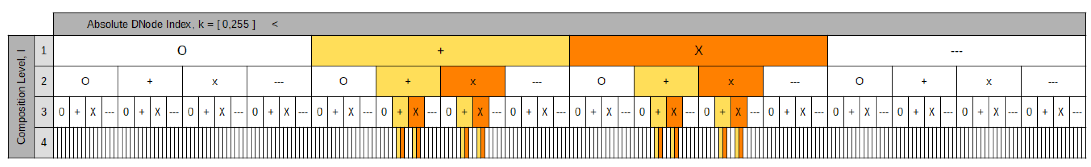
| sequential index of all DNodes in a specified composition level | |
| sequential index of all DNodes reachable from the current DNode | |
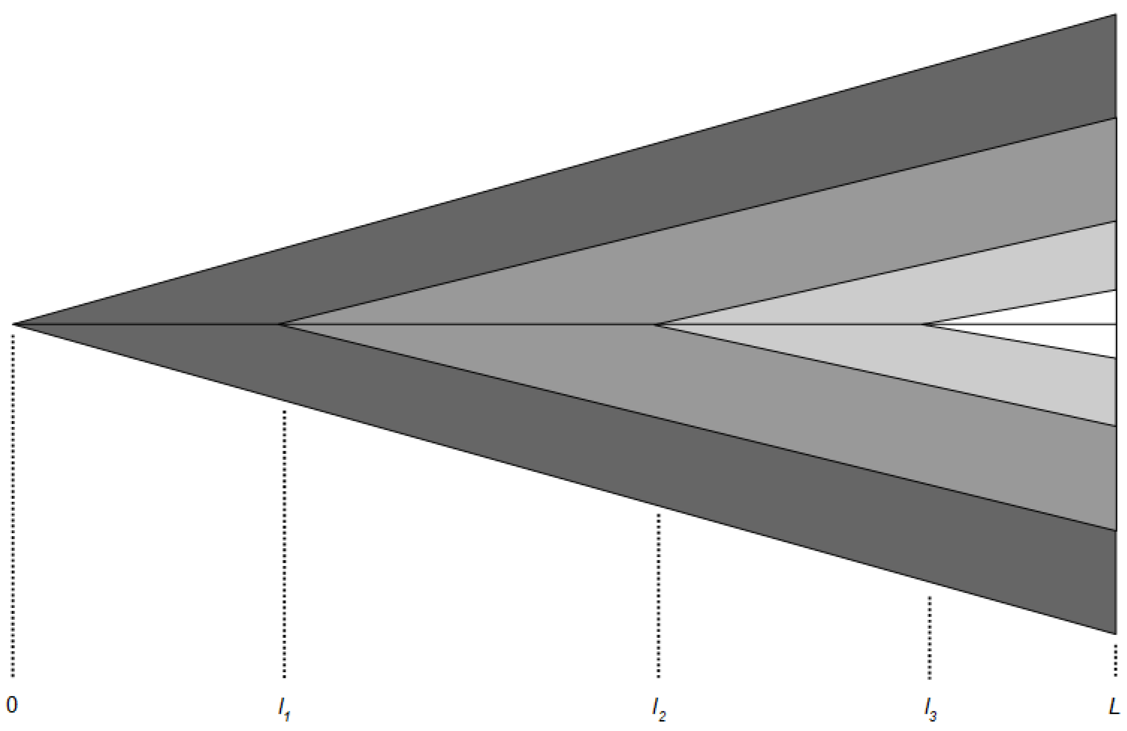
| l | composition level or index |
| current composition level, the reference level for next-DNode decisions | |
| L | number of composition levels needed to compose a DEP |
| n | number of retries needed to select the correct DNode |
| number of retries associated with a composition index | |
| normalized DSpace information | |
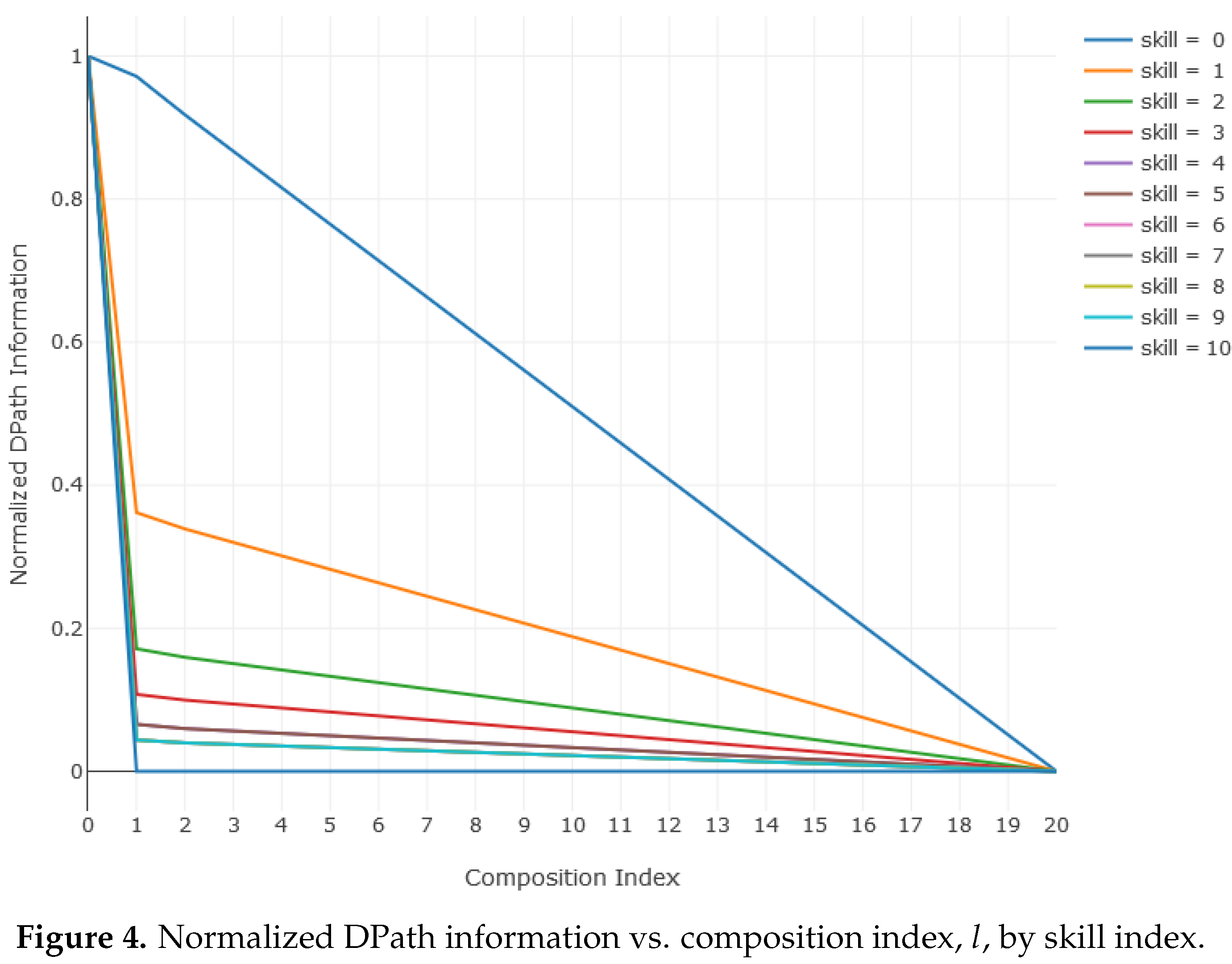
| normalized DPath information | |
| number of DNodes associated with a DSpace | |
| number of DNodes associated with a DPath | |
| p | general probability variable |
| probability that a DPath does not lead to a DEP, i.e., risk of project failure | |
| DPath success probability lower limit | |
| probability associated with a skill index value | |
| probability that a DPath leads to a DEP | |
| q | probability associated with DNode selection |
| Q | product of V and R |
| R | set of relations |
| r | member of the set of relations |
| index with range [0,10] that ranks an agent’s skill level, see | |
| t | test, a member of test set T |
| test result corresponding to test t | |
| T | set of tests |
| u | probability associated with vocabulary item selection |
| v | member of the set of vocabulary items |
| V | set of vocabulary items |
| test set result computed as the weighted sum of results of the test set’s members. | |
| w | weight applied to a test result, , when calculating a test set result |
| x | placeholder variable |
References
- Howard, M.; Lipner, S. The Security Development Lifecycle; Secure Software Deelopment, Microsoft Press: Redmond, WA, USA, 2006; p. 320. [Google Scholar]
- Microsoft. Simplified Implementation of the Microsoft SDL. Available online: https://www.microsoft.com/en-us/securityengineering/sdl/ (accessed on 3 May 2020).
- NIST Special Publication 800-37 Revision 2. Risk Management Framework for Information Systems and Organizations. Department of Commerce. p. 183. Available online: https://doi.org/10.6028/NIST.SP.800-37r2 (accessed on 23 May 2020).
- Systems Engineering Life Cycle Department of Homeland Security. p. 15. Available online: https://www.dhs.gov/sites/default/files/publications/Systems%20Engineering%20Life%20Cycle.pdf (accessed on 23 May 2020).
- Seal, D.; Farr, D.; Hatakeyama, J.; Haase, S. The System Engineering Vee is it Still Relevant in the Digital Age? In Proceedings of the NIST Model Based Enterprise Summit 2018, Gaithersburg, MD, USA, 4 April 2018; p. 10. [Google Scholar]
- FHWA. Systems Engineering for ITS Handbook—Section 3 What is Systems Engineering? Available online: https://ops.fhwa.dot.gov/publications/seitsguide/section3.htm (accessed on 3 May 2020).
- Modi, H.S.; Singh, N.K.; Chauhan, H.P. Comprehensive Analysis of Software Development Life Cycle Models. Int. Res. J. Eng. Technol. 2017, 4, 117–122. [Google Scholar]
- Sedmak, A. DoD Systems Engineering Policy, Guidance and Standardization. In Proceedings of the 19th Annual NDIA Systems Engineering Conference, Springfield, VA, USA, 26 October 2016; p. 21. Available online: https://ndiastorage.blob.core.usgovcloudapi.net/ndia/2016/systems/18925-AileenSedmak.pdf (accessed on 1 June 2020).
- Systems Engineering Plan Preparation Guide. Department of Defense. 2008, p. 96. Available online: Http://www.acqnotes.com/Attachments/Systems%20Engineering%20Plan%20Preparation%20Guide.pdf (accessed on 1 June 2020).
- Jolly, S. Systems Engineering: Roles and Responsibilities. In Proceedings of the NASA PI-Forum, Annapolis, MD, USA, 27 July 2011; p. 21. Available online: https://www.nasa.gov/pdf/580677main_02_Steve_Jolly_Systems_Engineering.pdf (accessed on 1 June 2020).
- Kaur, D.; Sharma, M. Classification Scheme for Software Reliability Models. In Artificial Intelligence and Evolutionary Computations in Engineering Systems, Advances in Intelligent Systems and Computing 394; Dash, S., Ed.; Springer: New Delhi, India, 2016; pp. 723–733. [Google Scholar] [CrossRef]
- Kruchten, P.; Nord, R.L.; Ozkaya, I. Managing Technical Debt: Reducing Friction in Software Development, 1st ed.; SEI Series in Software Engineering; Addison-Wesley Professional: Boston, MA, USA, 2019. [Google Scholar]
- Palepu, V.K.; Jones, J.A. Visualizing Constituent Behaviors within Executions. In Proceedings of the 2013 First IEEE Working Conference on Software Visualization (VISSOFT), Eindhoven, The Netherlands, 27–28 September 2013; pp. 1–4. [Google Scholar] [CrossRef]
- Palepu, V.K.; Jones, J.A. Revealing Runtime Features and Constituent Behaviors within Software. In Proceedings of the 2015 IEEE 3rd Working Conference on Software Visualization (VISSOFT), Bremen, Germany, 27–28 September 2015; pp. 86–95. [Google Scholar] [CrossRef]
- Gericke, K.; Blessing, L. Comparisons Of Design Methodologies And Process Models Across Disciplines: A Literature Review. In Proceedings of the International Conference On Engineering Design, ICED11, Lyngby/Copenhagen, Denmark, 15–18 August 2011; Technical University of Denmark: Lyngby, Denmark, 2011. [Google Scholar]
- Thakurta, R.; Mueller, B.; Ahlemann, F.; Hoffmann, D. The State of Design—A Comprehensive Literature Review to Chart the Design Science Research Discourse. In Proceedings of the 50th Hawaii International Conference on System Sciences, Hilton Waikoloa Village, HI, USA, 4–7 January 2017; pp. 4685–4694. [Google Scholar]
- Forlizzi, J.; Stolterman, E.; Zimmerman, J. From Design Research to Theory: Evidence of a Maturing Field. Korean Soc. Des. Sci. 2009, 9, 2889–2898. [Google Scholar]
- Antunes, R.; Gonzalez, V. A Production Model for Construction: A Theoretical Framework. Buildings 2015, 5, 209–228. [Google Scholar] [CrossRef]
- Vandenbrande, J. Transformative Design (TRADES). Available online: https://www.darpa.mil/program/transformative-design (accessed on 3 May 2020).
- Vandenbrande, J. Enabling Quantification of Uncertainty in Physical Systems (EQUiPS). Available online: https://www.darpa.mil/program/equips (accessed on 3 May 2020).
- Vandenbrande, J. Fundamental Design (FUN Design). Available online: https://www.darpa.mil/program/fundamental-design (accessed on 3 May 2020).
- Vandenbrande, J. Evolving Computers from Tools to Partners in Cyber-Physical System Design. Available online: https://www.darpa.mil/news-events/2019-08-02 (accessed on 3 May 2020).
- Ertas, A. Transdisciplinary Engineering Design Process; John Wiley & Sons, Inc.: Hoboken, NJ, USA, 2018; p. 818. [Google Scholar]
- Suh, N.P. Complexity Theory and Applications; Oxford University Press: Oxford, UK, 2005. [Google Scholar]
- Friedman, K. Theory Construction in Design Research. Criteria, Approaches, and Methods. In Proceedings of the 2002 Design Research Society International Conference, London, UK, 5–7 September 2002. [Google Scholar]
- Saunier, J.; Carrascosa, C.; Galland, S.; Patrick, S.K. Agent Bodies: An Interface Between Agent and Environment. In Agent Environments for Multi-Agent Systems IV, Lecture Notes in Computer Science; Weyns, D., Michel, F., Eds.; Springer: Cham, Switzerland, 2015; Volume 9068, pp. 25–40. [Google Scholar] [CrossRef]
- Heylighen, F.; Vidal, C. Getting Things Done: The Science Behind Stress-Free Productivity. Long Range Plan. 2008, 41, 585–605. [Google Scholar] [CrossRef]
- Eagleman, D. Incognito; Vintage Books: New York, NY, USA, 2011; p. 290. [Google Scholar]
- Wang, Y. On Contemporary Denotational Mathematics for Computational Intelligence. In Transactions on Computer Science II, LNCS 5150; Springer: Berlin/Heidelberg, Germany, 2008; pp. 6–29. [Google Scholar]
- Wang, Y. Using Process Algebra to Describe Human and Software Behaviors. Brain Mind 2003, 4, 199–213. [Google Scholar] [CrossRef]
- Wang, Y.; Tan, X.; Ngolah, C.F. Design and Implementation of an Autonomic Code Generator Based on RTPA. Int. J. Softw. Sci. Comput. Intell. 2010, 2, 44–65. [Google Scholar] [CrossRef]
- Park, B.K.; Kim, R.Y.C. Effort Estimation Approach through Extracting Use Cases via Informal Requirement Specifications. Appl. Sci. 2020, 10, 3044. [Google Scholar] [CrossRef]
- Qureshi, A.J.; Gericke, K.; Blessing, L. Design Process Commonalities in Transdisciplinary Design. In Proceedings of the International Conference on Engineering Design (ICED13), Seoul, Korea, 19–22 August 2013. [Google Scholar]
- Srinivasan, V.; Chakrabarti, A. SAPPhIRE—An Approach to Analysis and Synthesis. In Proceedings of the International Conference on Engineering Design (ICED09), Stanford, CA, USA, 24–27 August 2009. [Google Scholar]
- Reich, Y.; Subramanian, G.H. The PSI Matrix—A Framework and a Theory of Design. In Proceedings of the 21st International Conference on Engineering Design (ICED17), Vancouver, BC, Canada, 21–25 August 2017. [Google Scholar]
- Gericke, K.; Eckert, C.M.; Martin, S. What Do We Need To Say About A Design Method? In Proceedings of the 21st International Conference on Engineering Design (ICED17), Vancouver, BC, Canada, 21–25 August 2017. [Google Scholar]
- Gericke, K.; Eckert, C.M. The Long Road to Improvement in Modelling and Managing Engineering Design Processes. In Proceedings of the International Conference on Engineering Design (ICED15), Milan, Italy, 27–30 July 2015. [Google Scholar]
- Spacey, J. Risk Guide. Available online: https://simplicable.com/new/risk (accessed on 17 May 2020).
- Kendrick, T. Identifying and Managing Project Risk, 3rd ed.; American Management Association: New York, NY, USA, 2015. [Google Scholar]
- MITRE. Common Weakness Scoring System (CWSS™). Available online: https://cwe.mitre.org/cwss/cwss_v1.0.1.html (accessed on 3 May 2020).
- WhiteHat. Application Security Statistics Report; WhiteHat Security: San Jose, CA, USA, 2019; p. 34. [Google Scholar]
- Open Web Application Security Project. OWASP Risk Rating Methodology. Available online: https://owasp.org/www-community/OWASP_Risk_Rating_Methodology (accessed on 21 May 2020).
- Becker, G.M. A Practical Risk Management Approach. In PMI Global Congress 2004—North America, Anaheim, CA; Project Management Institute: Newtown Square, PA, USA, 2004; Available online: https://www.pmi.org/learning/library/practical-risk-management-approach-8248 (accessed on 3 May 2020).
- Rashid, A.; Chivers, H.; Danezis, G.; Lupu, E.; Martin, A. The Cyber Security Body of Knowledge; Centre, T.N.C.S., Ed.; University of Bristol: Bristol, UK, 2019; p. 834. [Google Scholar]
- Suh, N.P. Principles of Design; Oxford University Press: New York, NY, USA, 1990; p. 401. [Google Scholar]
- Vigo, R. Complexity over Uncertainty in Generalized Representational Information Theory (GRIT): A Structure-Sensitive General Theory of Information. Inf. Syst. Des. Intell. 2013, 4, 1. [Google Scholar] [CrossRef]
- Shannon, C.E. A Mathematical Theory of Communication. Bell Syst. Tech. J. 1948, 27, 379–423. [Google Scholar] [CrossRef]
- Naik, K.; Tripathy, P. Software Testing and Quality Assurance; John Wiley & Sons, Inc.: Hoboken, NJ, USA, 2008; p. 616. [Google Scholar]
- RTI. The Economic Impacts of Inadequate Infrastructure for Software Testing; RTI: Gaithersburg, MD, USA, 2002. [Google Scholar]
- McConnell, S. Code Complete; Microsoft Press: Redmond, WA, USA, 1993. [Google Scholar]


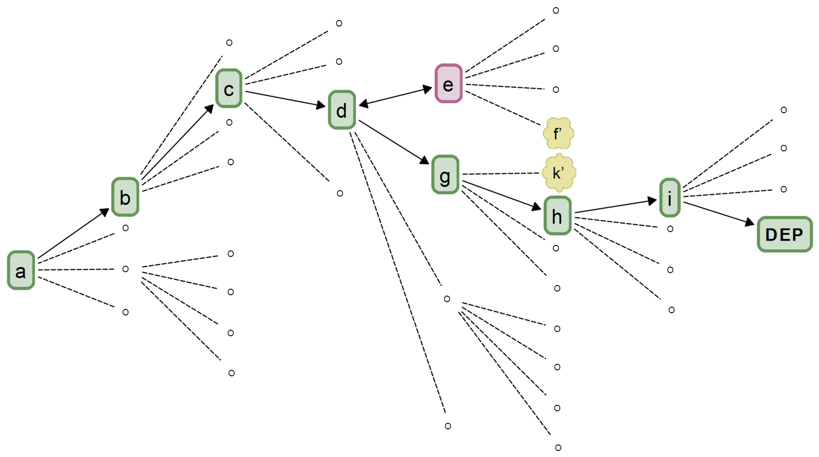
| DPath Type | DPath Index (Traversal and Navigation) | |||||||||||||||
|---|---|---|---|---|---|---|---|---|---|---|---|---|---|---|---|---|
| 0 | 1 | 2 | 3 | 4 | 5 | 6 | 7 | 8 | 9 | 10 | 11 | 12 | 13 | 14 | 15 | |
| Actual | a | b | c | d | e | f’ | e | d | g | k’ | g | h’ | g | h | i | DEP |
| Net | a | b | c | d | g | h | i | DEP | ||||||||
| Current DNode | Next DNode Options | ||||
|---|---|---|---|---|---|
| (l,ka) | k | ν(l+1,k) | p(l+1,k) | h(l+1,k) | Selected |
| (0,~) | 0 | 0.00 | 0.2500 | 2.0000 | |
| 1 | 1.00 | 1.0000 | 0.0000 | Y | |
| 2 | 0.00 | 0.2500 | 2.0000 | ||
| 3 | 0.00 | 0.2500 | 2.0000 | ||
| (1,1) | 0 | 0.00 | 0.2500 | 2.0000 | |
| 1 | 1.00 | 1.0000 | 0.0000 | Y | |
| 2 | 0.00 | 0.2500 | 2.0000 | ||
| 3 | 0.00 | 0.2500 | 2.0000 | ||
| (2,5) | 0 | 0.00 | 0.2500 | 2.0000 | |
| 1 | 1.00 | 1.0000 | 0.0000 | Y | |
| 2 | 0.00 | 0.2500 | 2.0000 | ||
| 3 | 0.00 | 0.2500 | 2.0000 | ||
| (3,21) | 0 | 0.00 | 0.2500 | 2.0000 | |
| 1 | 1.00 | 1.0000 | 0.0000 | Y | |
| 2 | 0.00 | 0.2500 | 2.0000 | ||
| 3 | 0.00 | 0.2500 | 2.0000 | ||
| Composition Index (l) | |||||||||||||||||||||
|---|---|---|---|---|---|---|---|---|---|---|---|---|---|---|---|---|---|---|---|---|---|
| Test Set | DPath Index | 0 | 1 | 2 | 3 | 4 | |||||||||||||||
| k | ν(l,k) | p(l,k) | h(l,k) | k | ν(l,k) | p(l,k) | h(l,k) | k | ν(l,k) | p(l,k) | h(l,k) | k | ν(l,k) | p(l,k) | h(l,k) | k | ν(l,k) | p(l,k) | h(l,k) | ||
| 0 | 0 | ~ | ~ | 0.25 | 2.00 | 1 | 1.00 | 1.00 | 0.00 | 5 | 1.00 | 1.00 | 0.00 | 21 | 1.00 | 1.00 | 0.00 | 85 | 1.00 | 1.00 | 0.00 |
| Others | ~ | ~ | 0.25 | 2.00 | — | 0.00 | 0.25 | 2.00 | — | 0.00 | 0.25 | 2.00 | — | 0.00 | 0.25 | 2.00 | — | 0.00 | 0.25 | 2.00 | |
| 1 | 0 | ~ | ~ | 0.25 | 2.00 | 1 | 1.00 | 1.00 | 0.00 | 5 | 1.00 | 1.00 | 0.00 | 21 | 1.00 | 1.00 | 0.00 | 85 | 1.00 | 1.00 | 0.00 |
| 1 | ~ | ~ | 0.25 | 2.00 | 1 | 1.00 | 1.00 | 0.00 | 5 | 1.00 | 1.00 | 0.00 | 21 | 1.00 | 1.00 | 0.00 | 86 | 0.83 | 0.87 | 0.19 | |
| 2 | ~ | ~ | 0.25 | 2.00 | 1 | 1.00 | 1.00 | 0.00 | 5 | 1.00 | 1.00 | 0.00 | 22 | 0.83 | 0.87 | 0.20 | 89 | 1.00 | 1.00 | 0.00 | |
| 3 | ~ | ~ | 0.25 | 2.00 | 1 | 1.00 | 1.00 | 0.00 | 5 | 1.00 | 1.00 | 0.00 | 22 | 0.83 | 0.87 | 0.20 | 90 | 0.83 | 0.87 | 0.20 | |
| 4 | ~ | ~ | 0.25 | 2.00 | 1 | 1.00 | 1.00 | 0.00 | 6 | 0.83 | 0.87 | 0.20 | 25 | 1.00 | 1.00 | 0.00 | 101 | 1.00 | 1.00 | 0.00 | |
| 5 | ~ | ~ | 0.25 | 2.00 | 1 | 1.00 | 1.00 | 0.00 | 6 | 0.83 | 0.87 | 0.20 | 25 | 1.00 | 1.00 | 0.00 | 102 | 0.83 | 0.87 | 0.20 | |
| 6 | ~ | ~ | 0.25 | 2.00 | 1 | 1.00 | 1.00 | 0.00 | 6 | 0.83 | 0.87 | 0.20 | 26 | 0.83 | 0.87 | 0.20 | 105 | 1.00 | 1.00 | 0.00 | |
| 7 | ~ | ~ | 0.25 | 2.00 | 1 | 1.00 | 1.00 | 0.00 | 6 | 0.83 | 0.87 | 0.20 | 26 | 0.83 | 0.87 | 0.20 | 106 | 0.83 | 0.87 | 0.20 | |
| 8 | ~ | ~ | 0.25 | 2.00 | 2 | 0.83 | 0.87 | 0.20 | 9 | 1.00 | 1.00 | 0.00 | 37 | 1.00 | 1.00 | 0.00 | 149 | 1.00 | 1.00 | 0.00 | |
| 9 | ~ | ~ | 0.25 | 2.00 | 2 | 0.83 | 0.87 | 0.20 | 9 | 1.00 | 1.00 | 0.00 | 37 | 1.00 | 1.00 | 0.00 | 150 | 0.83 | 0.87 | 0.20 | |
| 10 | ~ | ~ | 0.25 | 2.00 | 2 | 0.83 | 0.87 | 0.20 | 9 | 1.00 | 1.00 | 0.00 | 38 | 0.83 | 0.87 | 0.20 | 153 | 1.00 | 1.00 | 0.00 | |
| 11 | ~ | ~ | 0.25 | 2.00 | 2 | 0.83 | 0.87 | 0.20 | 9 | 1.00 | 1.00 | 0.00 | 38 | 0.83 | 0.87 | 0.20 | 154 | 0.83 | 0.87 | 0.20 | |
| 12 | ~ | ~ | 0.25 | 2.00 | 2 | 0.83 | 0.87 | 0.20 | 10 | 0.83 | 0.87 | 0.20 | 41 | 1.00 | 1.00 | 0.00 | 165 | 1.00 | 1.00 | 0.00 | |
| 13 | ~ | ~ | 0.25 | 2.00 | 2 | 0.83 | 0.87 | 0.20 | 10 | 0.83 | 0.87 | 0.20 | 41 | 1.00 | 1.00 | 0.00 | 166 | 0.83 | 0.87 | 0.20 | |
| 14 | ~ | ~ | 0.25 | 2.00 | 2 | 0.83 | 0.87 | 0.20 | 10 | 0.83 | 0.87 | 0.20 | 42 | 0.83 | 0.87 | 0.20 | 169 | 1.00 | 1.00 | 0.00 | |
| 15 | ~ | ~ | 0.25 | 2.00 | 2 | 0.83 | 0.87 | 0.20 | 10 | 0.83 | 0.87 | 0.20 | 42 | 0.83 | 0.87 | 0.20 | 170 | 0.83 | 0.87 | 0.20 | |
| Others | ~ | ~ | 0.25 | 2.00 | — | 0.00 | 0.25 | 2.00 | — | 0.00 | 0.25 | 2.00 | — | 0.00 | 0.25 | 2.00 | — | 0.00 | 0.25 | 2.00 | |
| Test Set | DPath Index | Information | Probability | ||
|---|---|---|---|---|---|
| DPath | Minimum | Success | Risk | ||
| 0 | 0 | 0.00 | 0.00 | 1.00 | 0.00 |
| Others | 0.00 | 1.00 | 0.00 | ||
| 1 | 0 | 0.00 | 0.00 | 1.00 | 0.00 |
| 1 | 0.19 | 0.87 | 0.13 | ||
| 2 | 0.20 | 0.87 | 0.13 | ||
| 3 | 0.39 | 0.76 | 0.24 | ||
| 4 | 0.20 | 0.87 | 0.13 | ||
| 5 | 0.39 | 0.76 | 0.24 | ||
| 6 | 0.39 | 0.76 | 0.24 | ||
| 7 | 0.59 | 0.66 | 0.34 | ||
| 8 | 0.20 | 0.87 | 0.13 | ||
| 9 | 0.39 | 0.76 | 0.24 | ||
| 10 | 0.39 | 0.76 | 0.24 | ||
| 11 | 0.59 | 0.66 | 0.34 | ||
| 12 | 0.39 | 0.76 | 0.24 | ||
| 13 | 0.59 | 0.66 | 0.34 | ||
| 14 | 0.59 | 0.66 | 0.34 | ||
| 15 | 0.79 | 0.58 | 0.42 | ||
| Others | 8.00 | 0.00 | 1.00 | ||
| DPath | Information | Probability | ||
|---|---|---|---|---|
| Actual | Scaled | Success | Risk | |
| 0 | 3021.351 | 1.07 | 0.48 | 0.52 |
| 1 | 8824.484 | 3.12 | 0.11 | 0.89 |
| 2 | 5104.543 | 1.81 | 0.29 | 0.71 |
| 3 | 8669.417 | 3.07 | 0.12 | 0.88 |
| 4 | 5855.308 | 2.07 | 0.24 | 0.76 |
| 5 | 7499.249 | 2.65 | 0.16 | 0.84 |
| 6 | 498.490 | 1.45 | 0.37 | 0.63 |
| 7 | 644.061 | 0.23 | 0.85 | 0.15 |
| 8 | 6843.825 | 2.42 | 0.19 | 0.81 |
| 9 | 1621.288 | 0.57 | 0.67 | 0.33 |
| 10 | 5426.940 | 1.92 | 0.26 | 0.74 |
| 11 | 6042.189 | 2.14 | 0.23 | 0.77 |
| 12 | 7838.449 | 2.77 | 0.15 | 0.85 |
| 13 | 8574.182 | 3.03 | 0.12 | 0.88 |
| 14 | 5791.182 | 2.05 | 0.24 | 0.76 |
| 15 | 9390.285 | 3.32 | 0.10 | 0.90 |
| 16 | 315.768 | 0.11 | 0.93 | 0.07 |
© 2020 by the authors. Licensee MDPI, Basel, Switzerland. This article is an open access article distributed under the terms and conditions of the Creative Commons Attribution (CC BY) license (http://creativecommons.org/licenses/by/4.0/).
Share and Cite
Denard, S.; Ertas, A.; Mengel, S.; Ekwaro-Osire, S. Development Cycle Modeling: Process Risk. Appl. Sci. 2020, 10, 5082. https://doi.org/10.3390/app10155082
Denard S, Ertas A, Mengel S, Ekwaro-Osire S. Development Cycle Modeling: Process Risk. Applied Sciences. 2020; 10(15):5082. https://doi.org/10.3390/app10155082
Chicago/Turabian StyleDenard, Samuel, Atila Ertas, Susan Mengel, and Stephen Ekwaro-Osire. 2020. "Development Cycle Modeling: Process Risk" Applied Sciences 10, no. 15: 5082. https://doi.org/10.3390/app10155082
APA StyleDenard, S., Ertas, A., Mengel, S., & Ekwaro-Osire, S. (2020). Development Cycle Modeling: Process Risk. Applied Sciences, 10(15), 5082. https://doi.org/10.3390/app10155082