Real-Time Visual Tracking of Moving Targets Using a Low-Cost Unmanned Aerial Vehicle with a 3-Axis Stabilized Gimbal System


Abstract
Featured Application
Abstract
1. Introduction
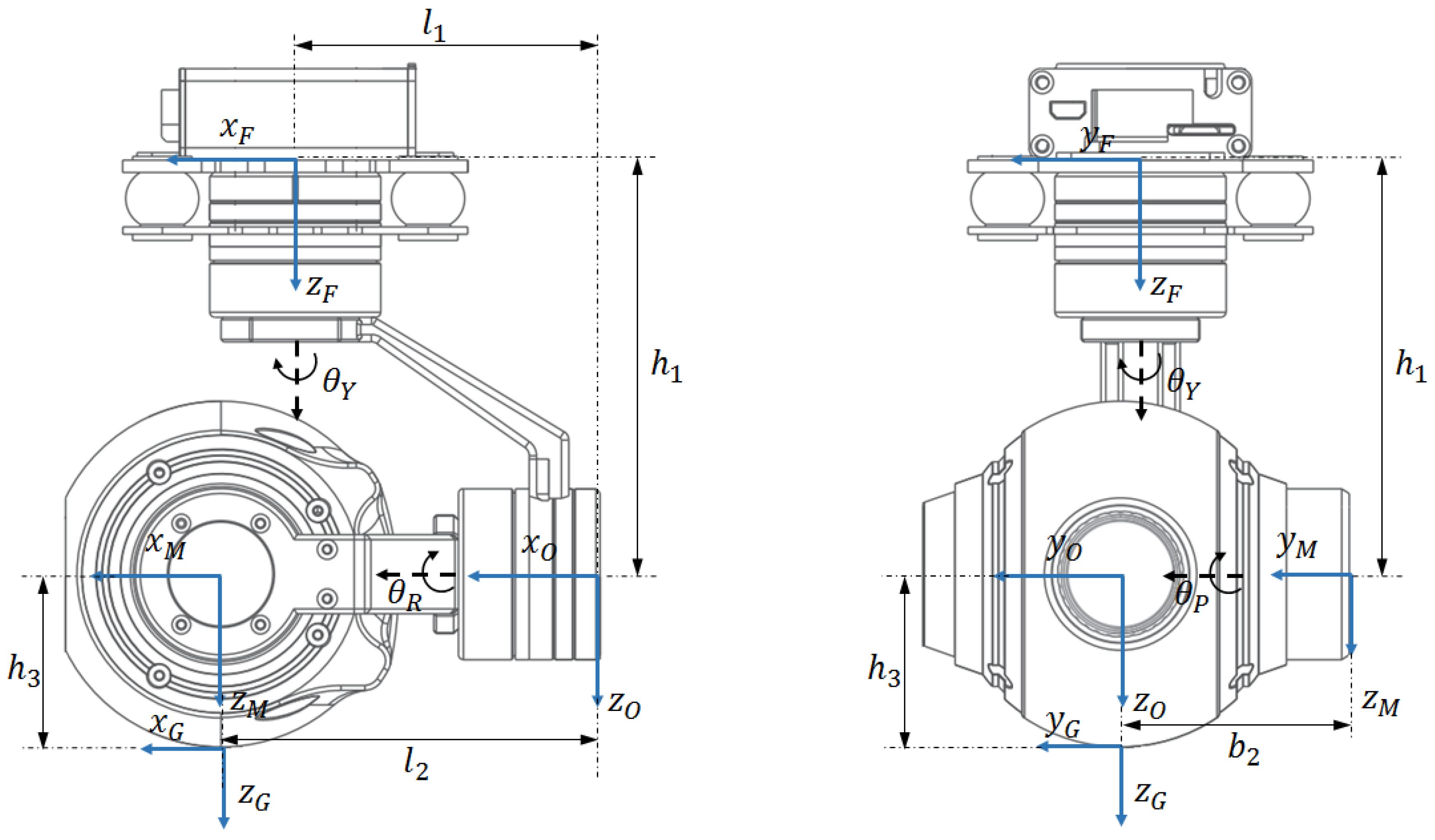
2. Gimbal System
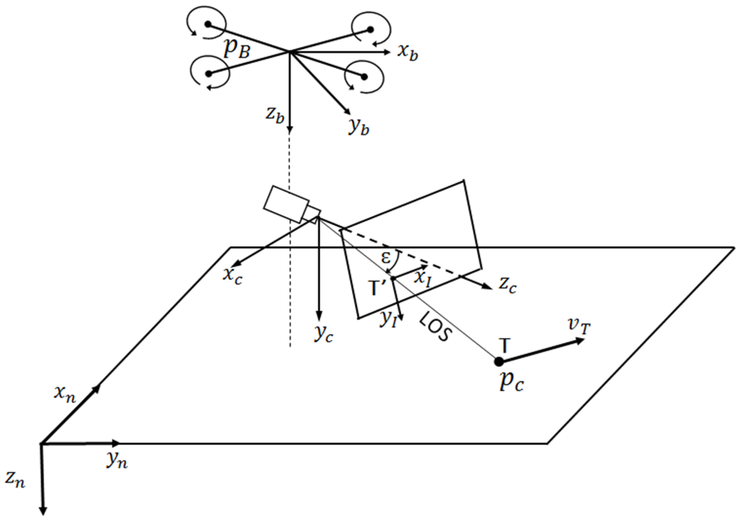
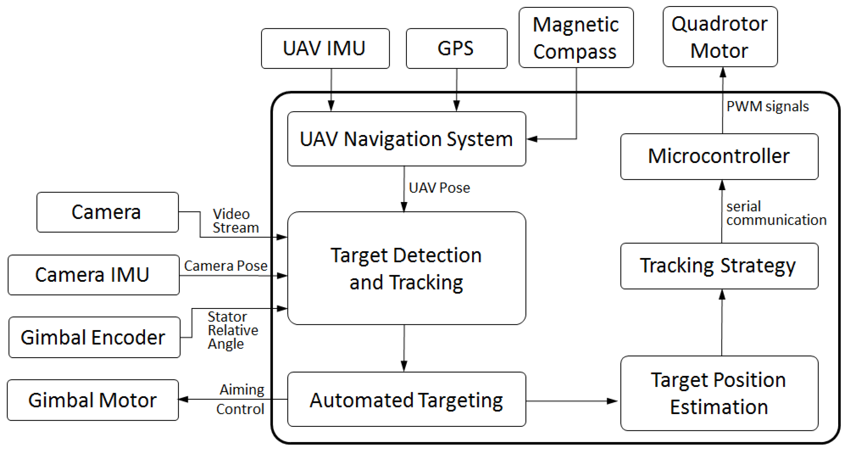
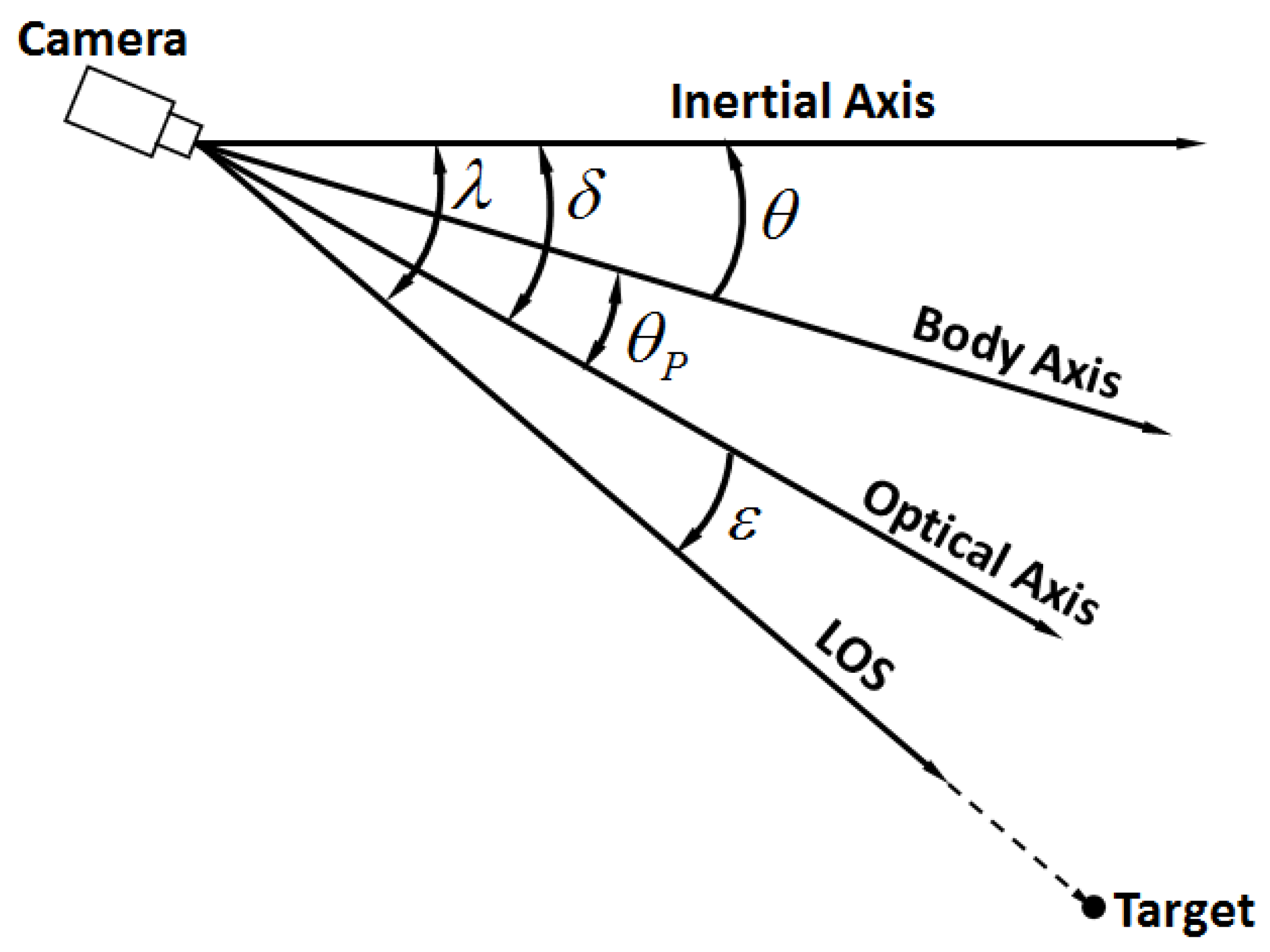
2.1. Problem Formulation and System Architecture
2.2. Kinematics of the Gimbal System
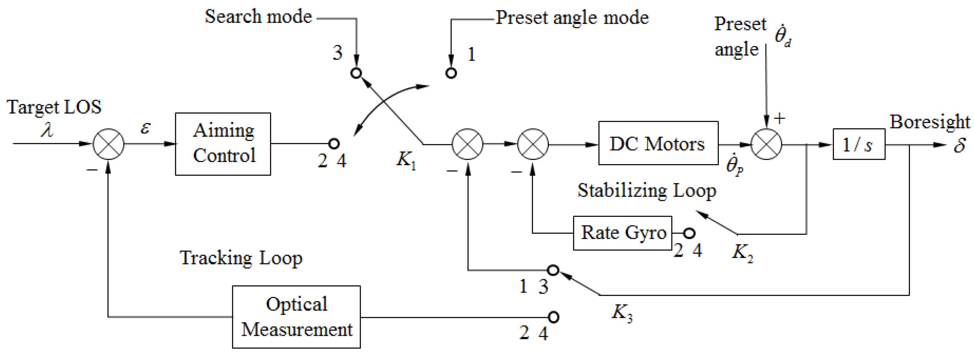
2.3. Stabilization and Aiming
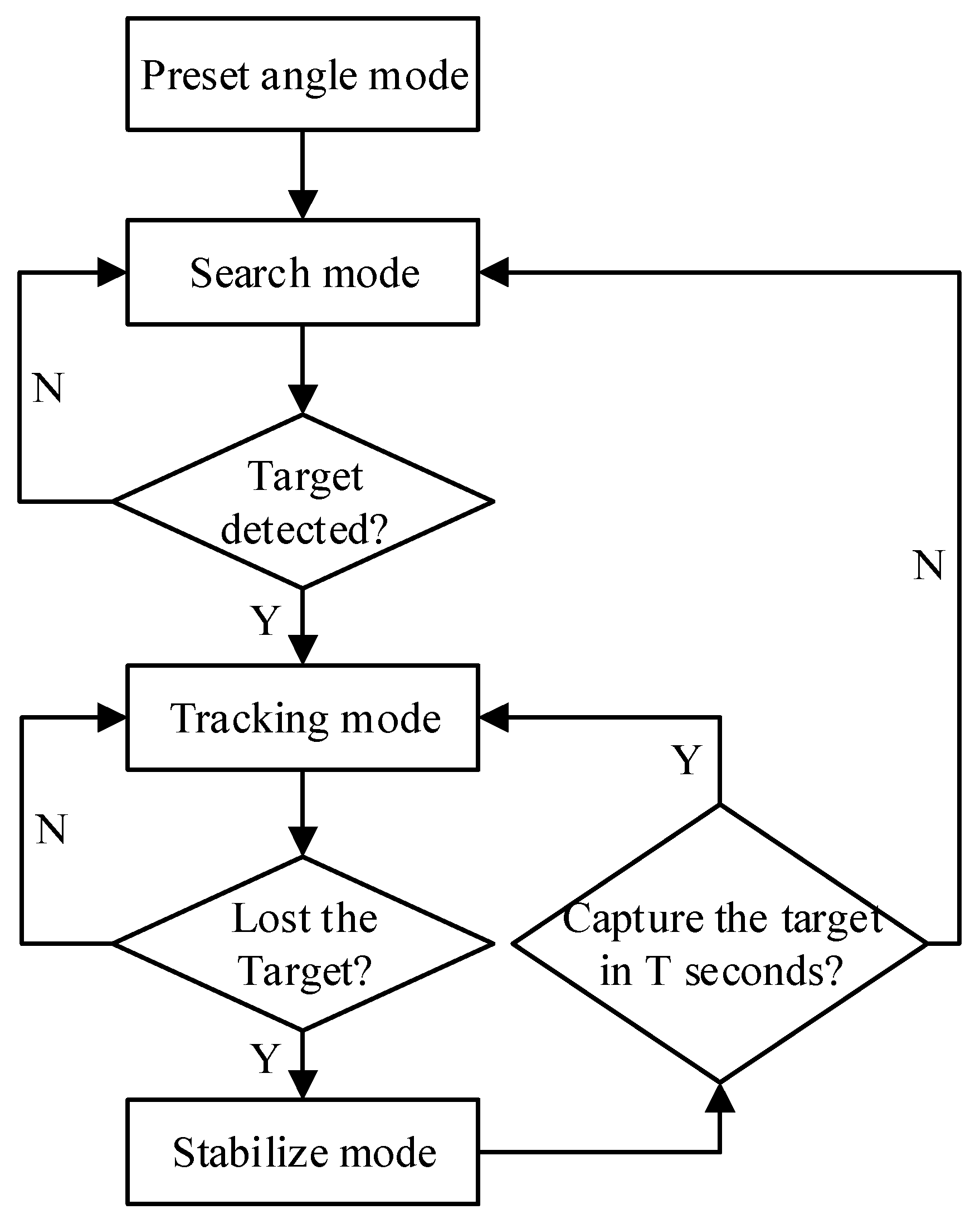
3. Target Tracking
3.1. KCF Tracker
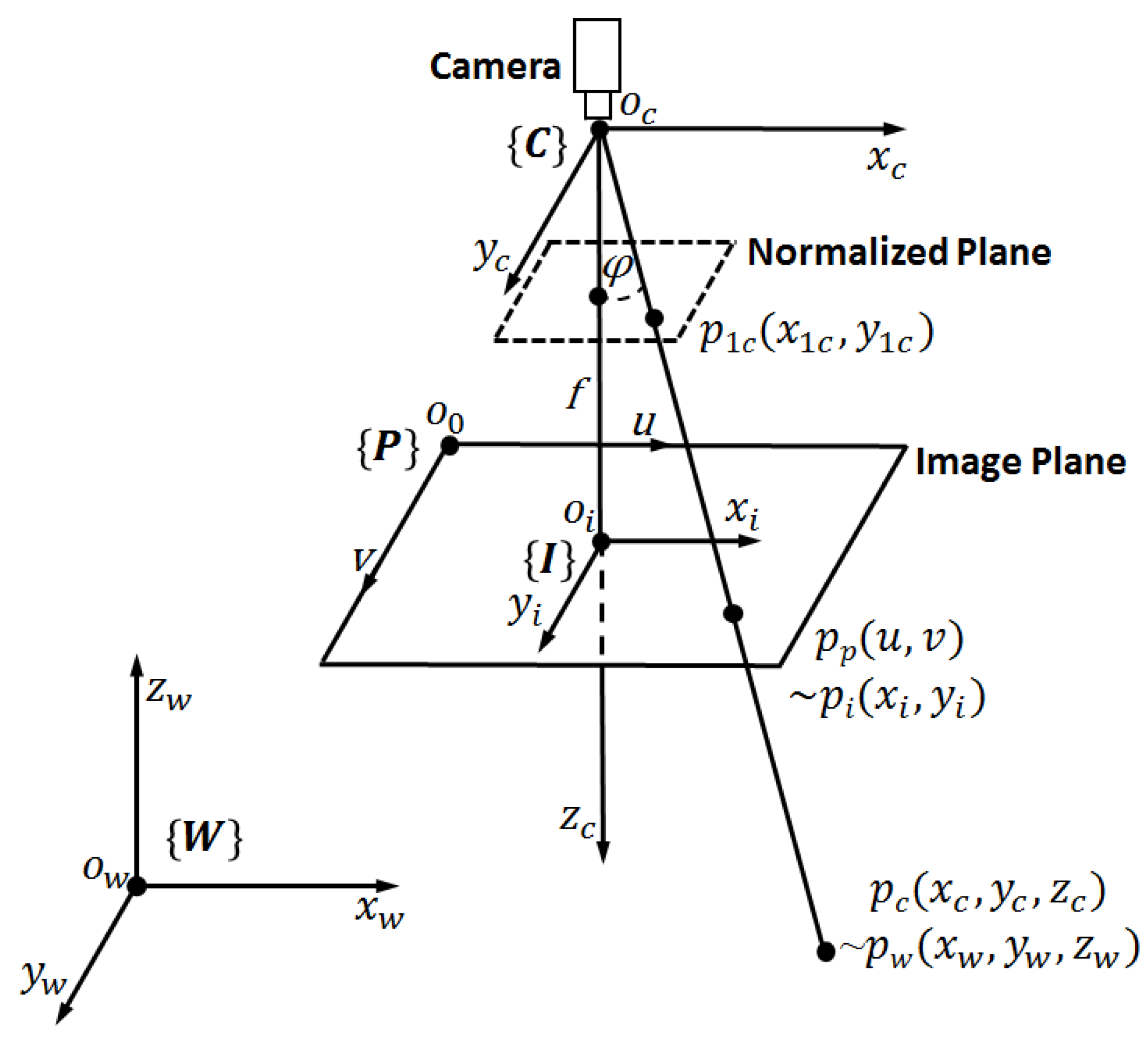
3.2. Target Localization
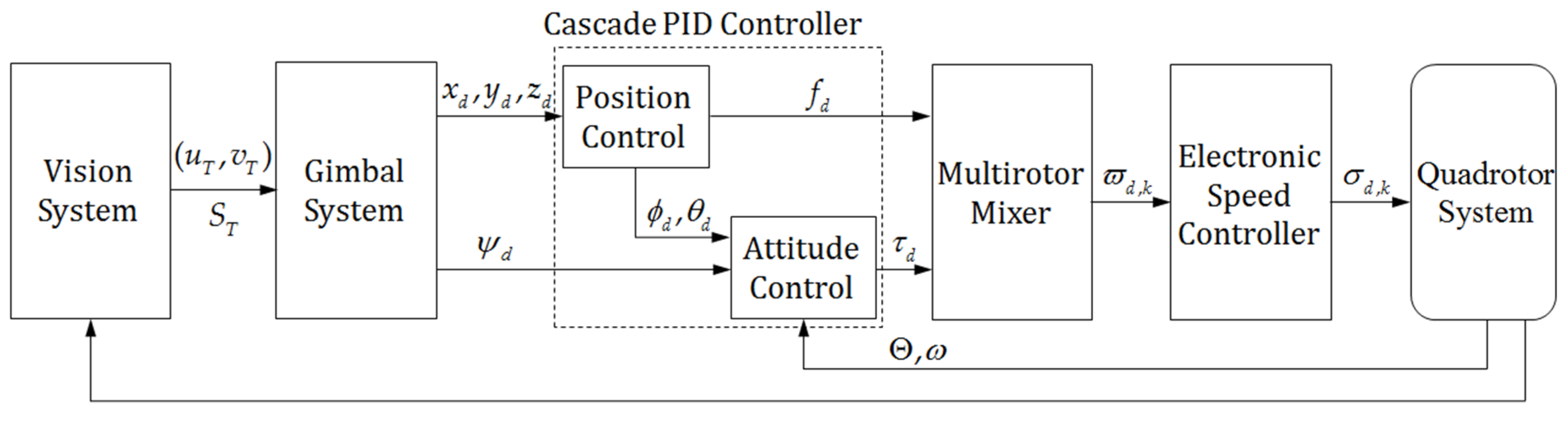
4. Flight Control Algorithm
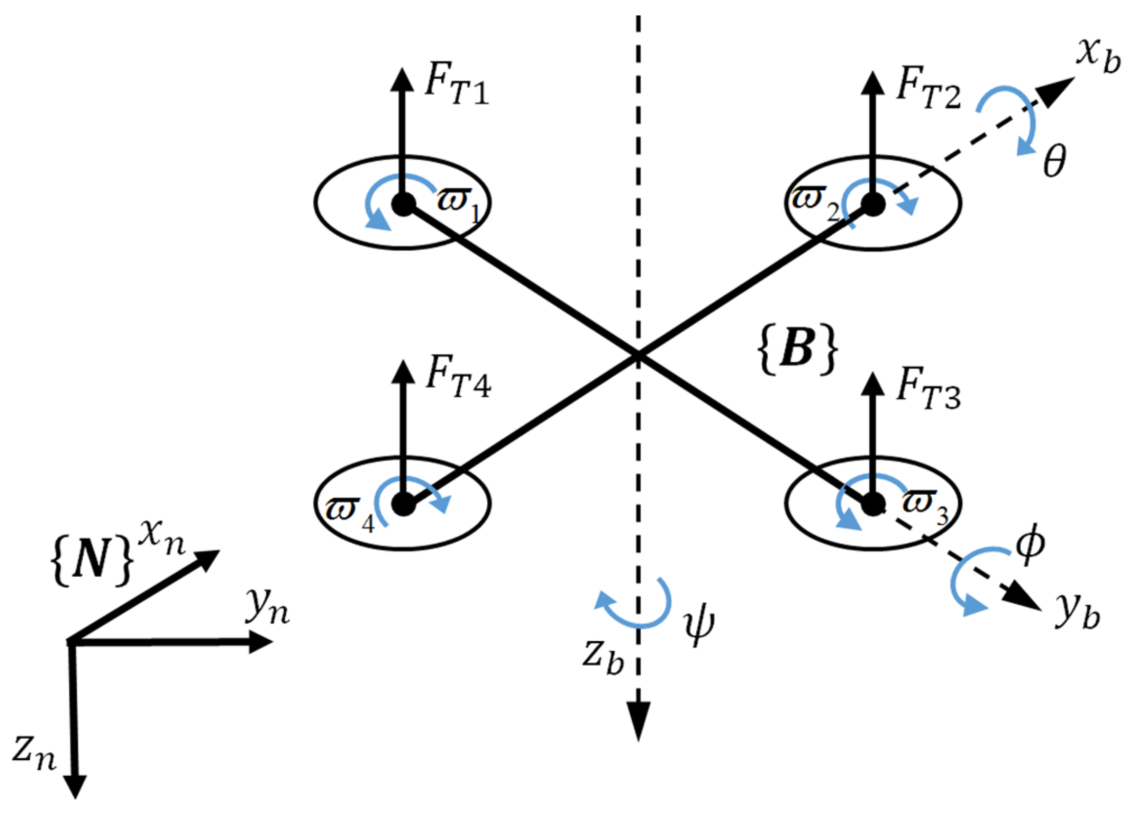
4.1. UAV Dynamic Model
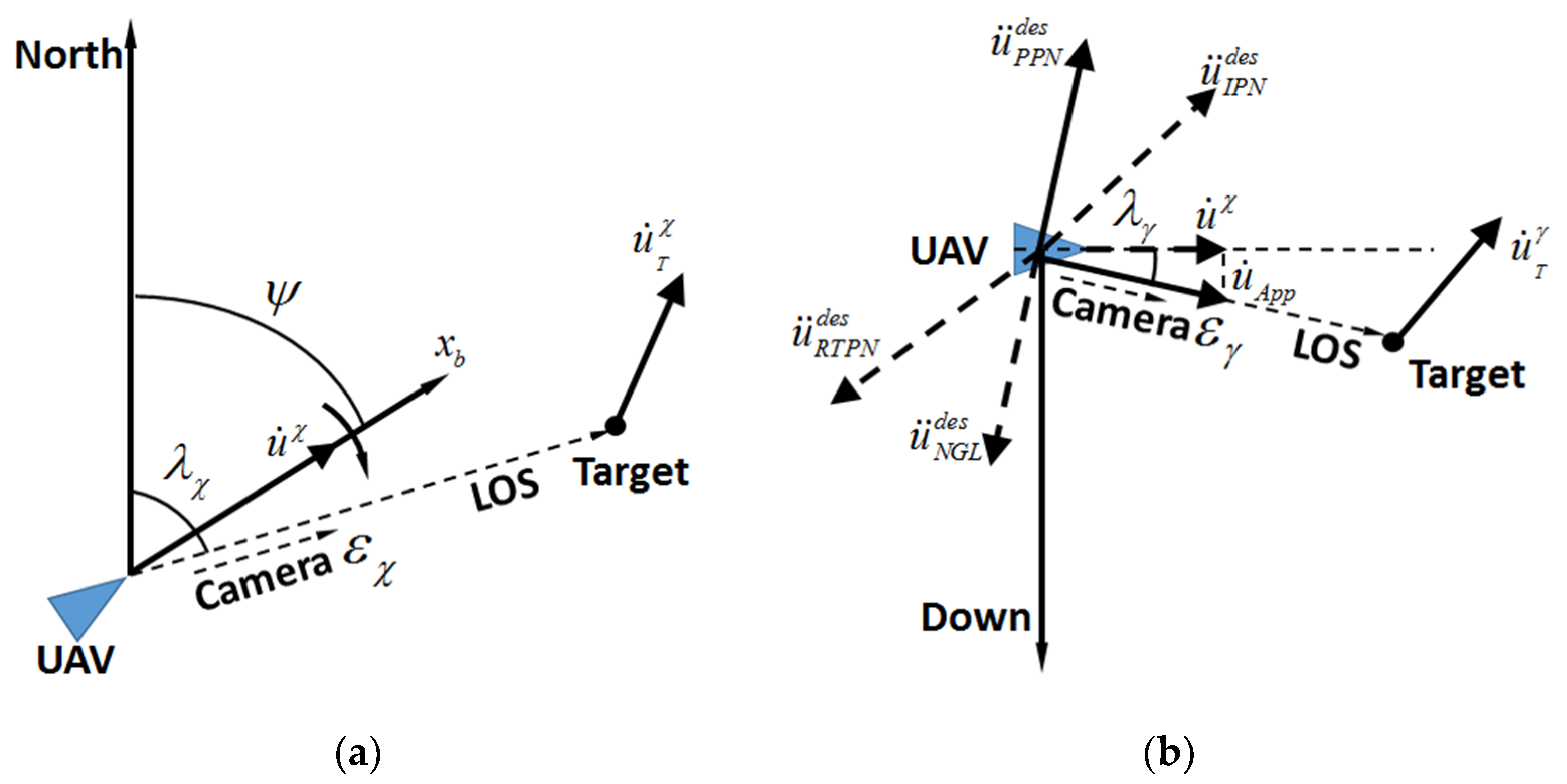
4.2. Tracking Strategy
4.3. Flight Control System
5. Experiments and Results
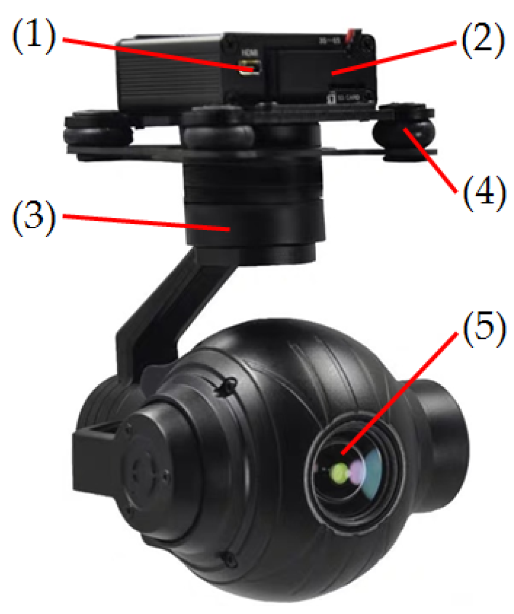
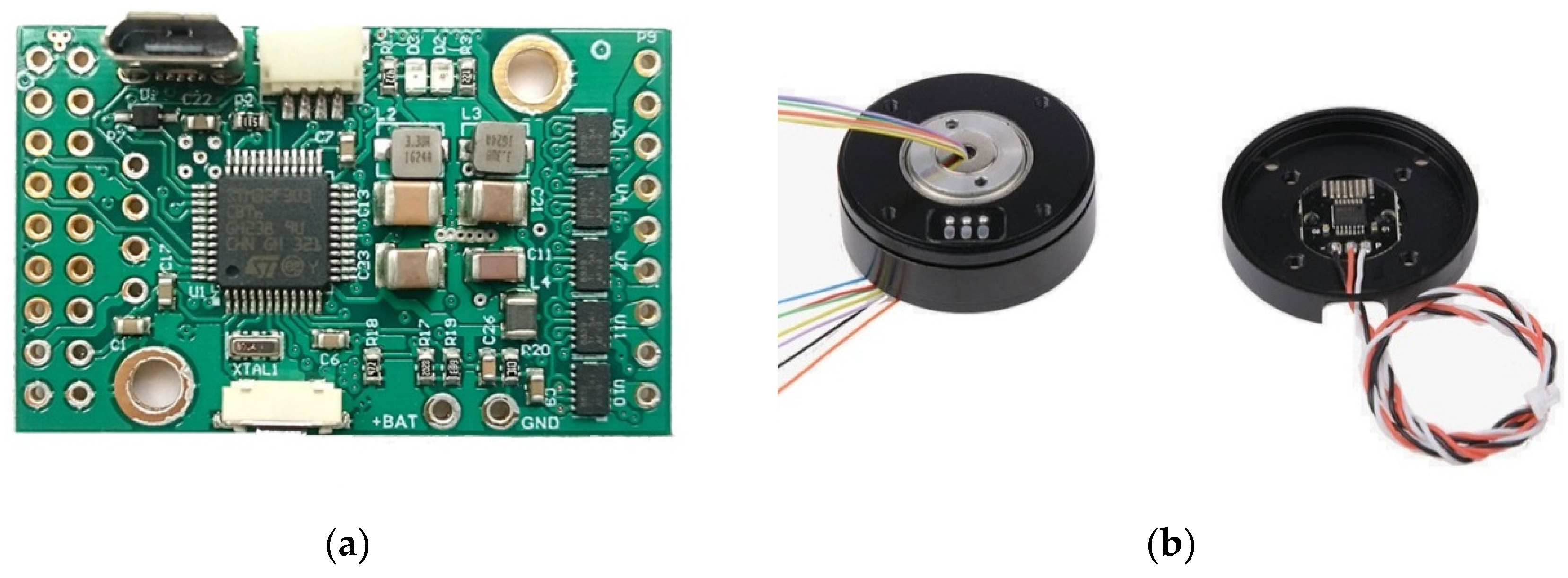
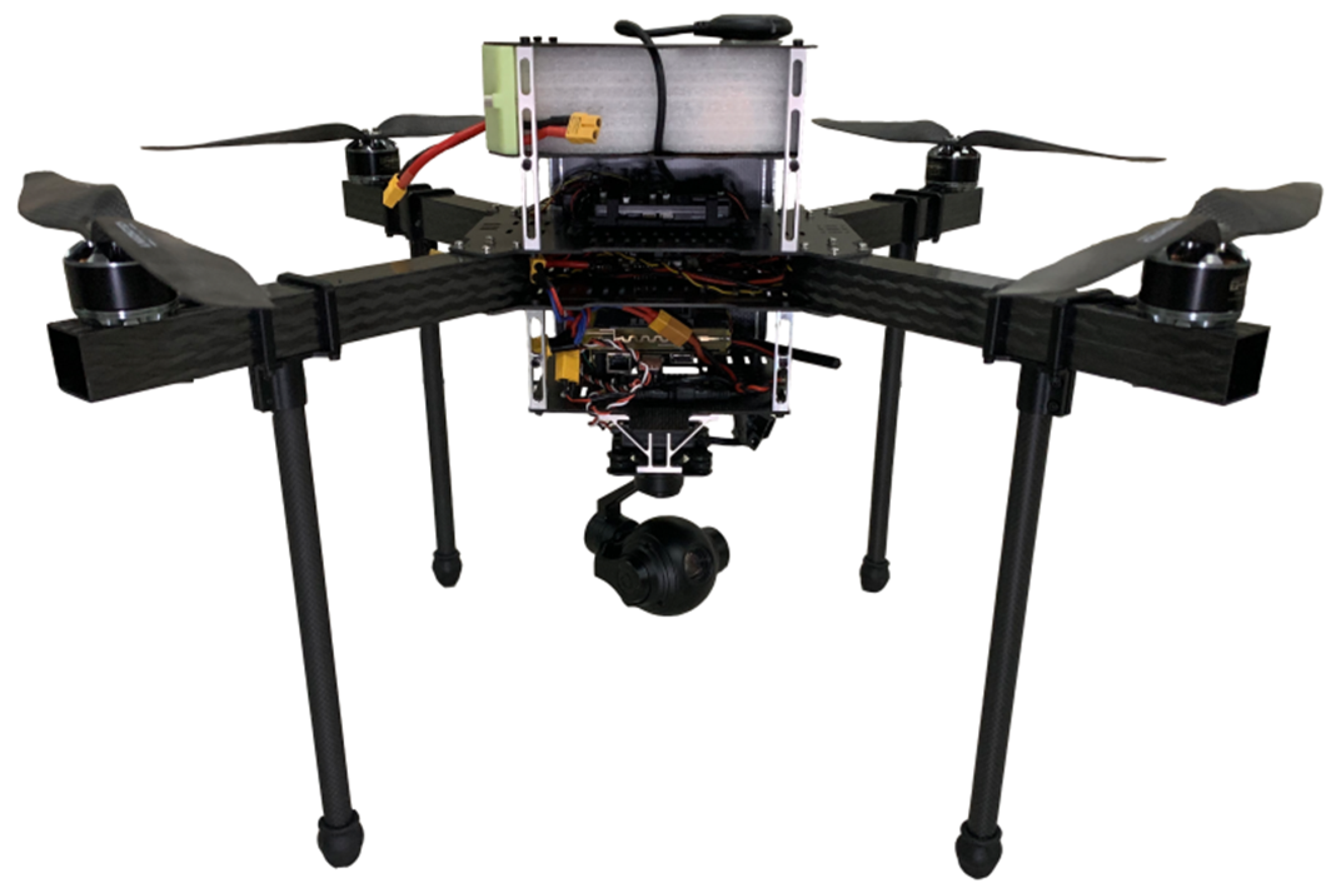
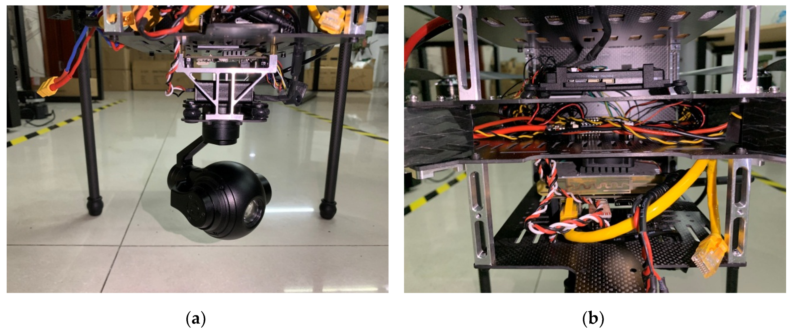
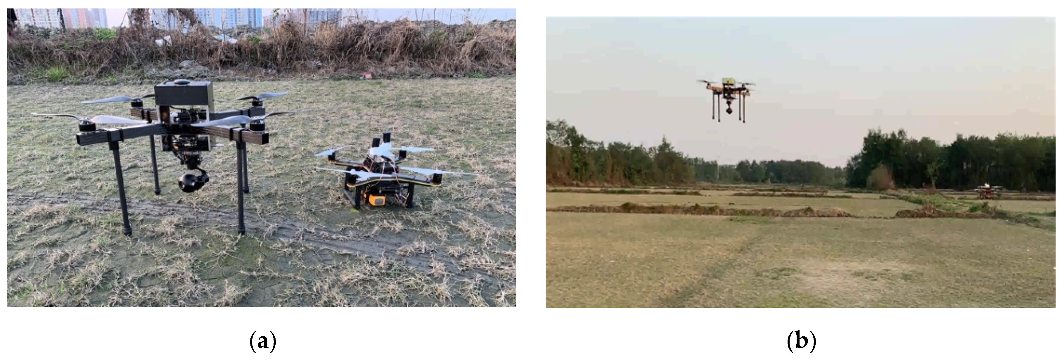
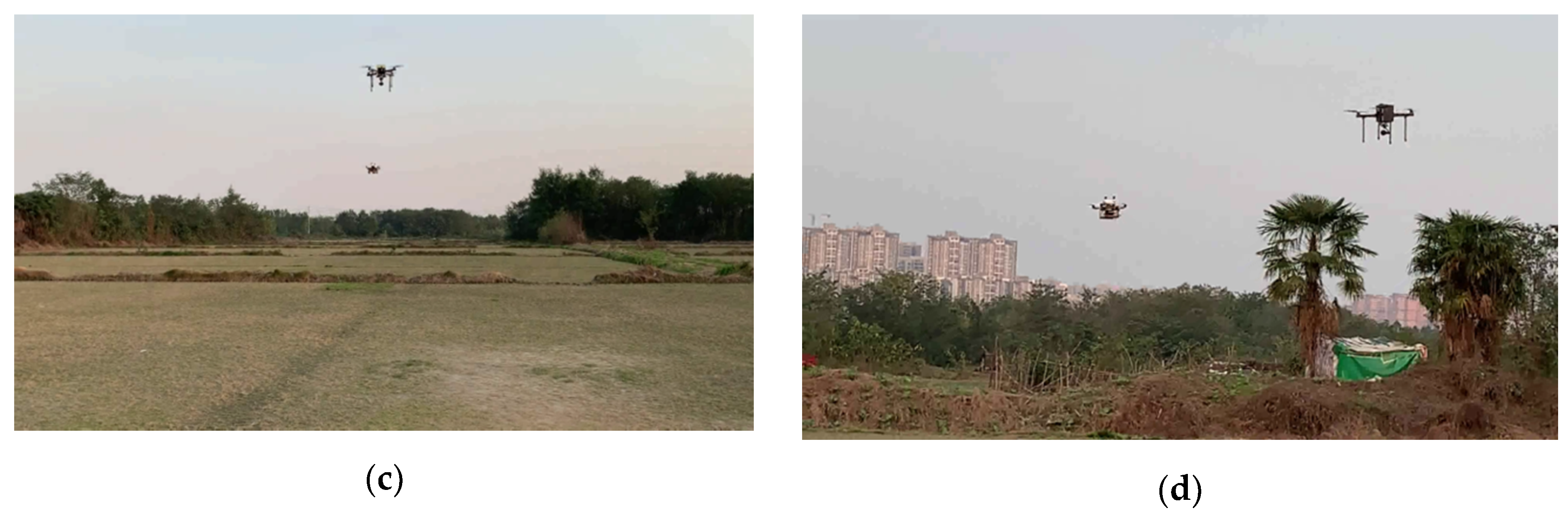
5.1. Experimental Setup
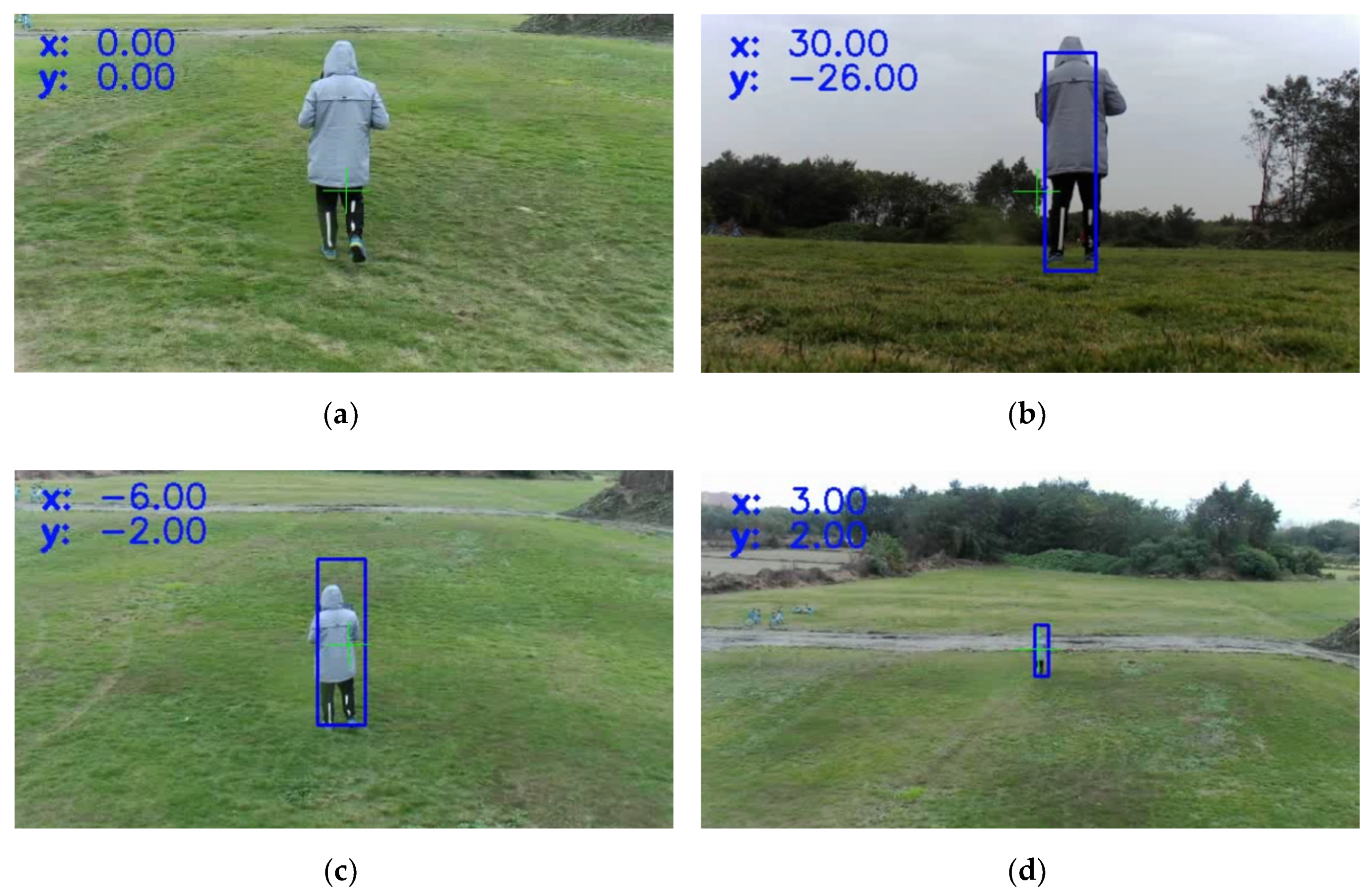
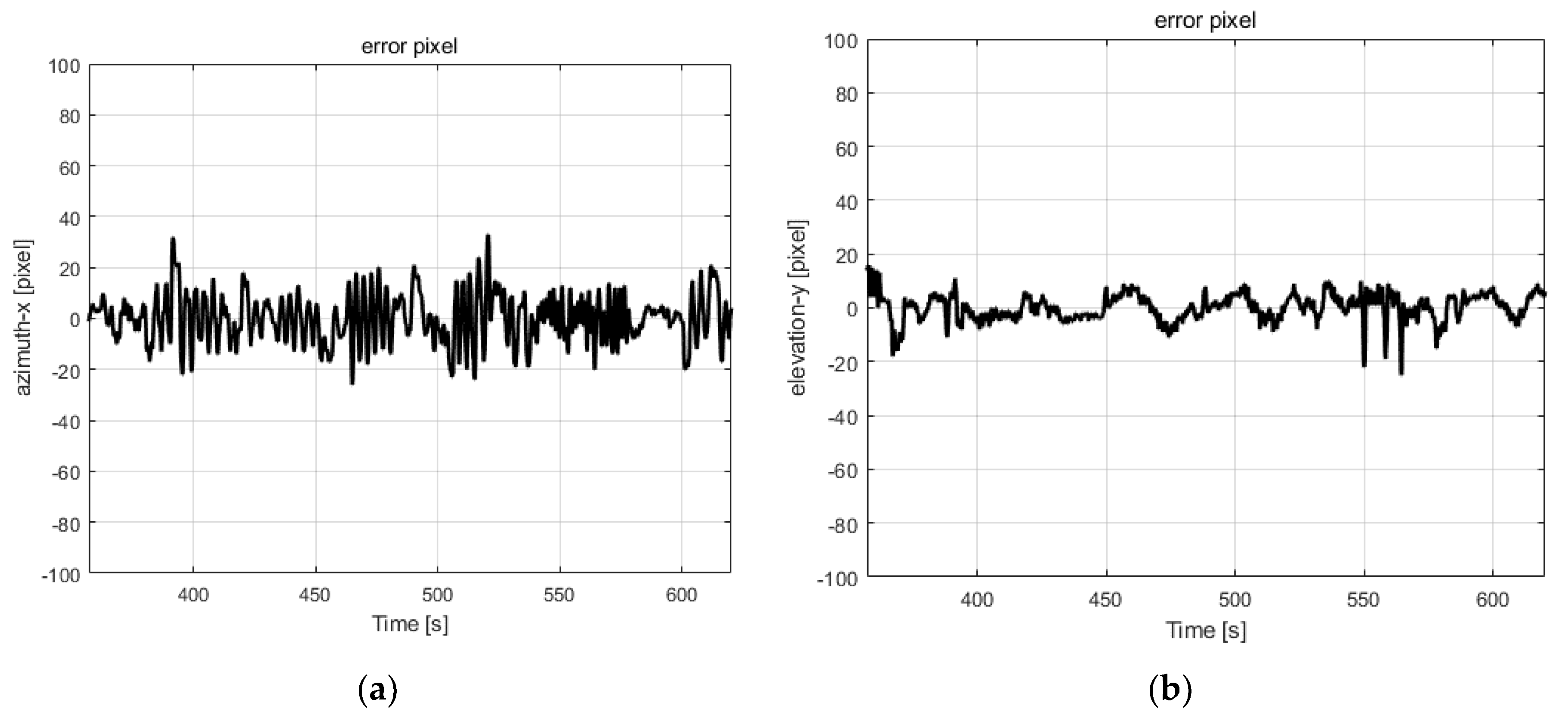
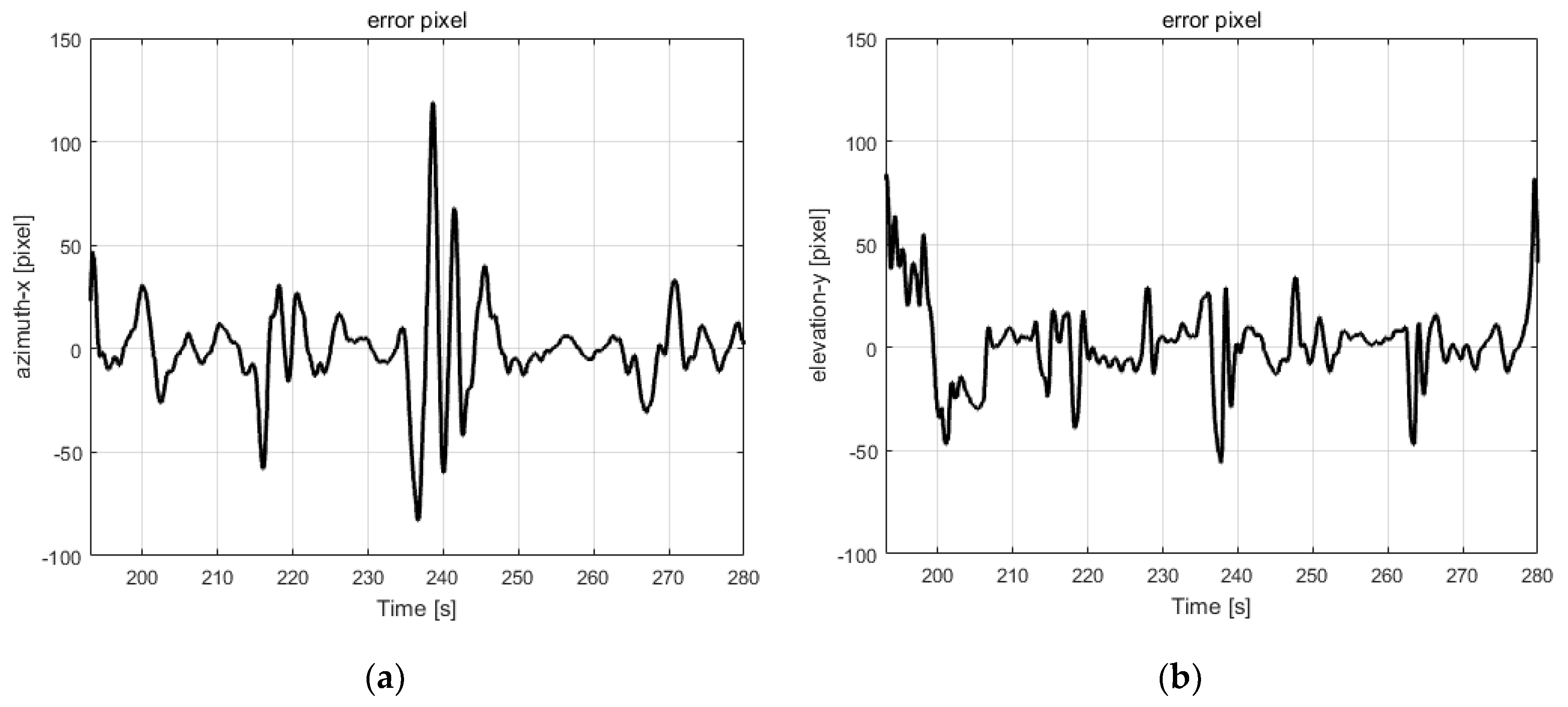
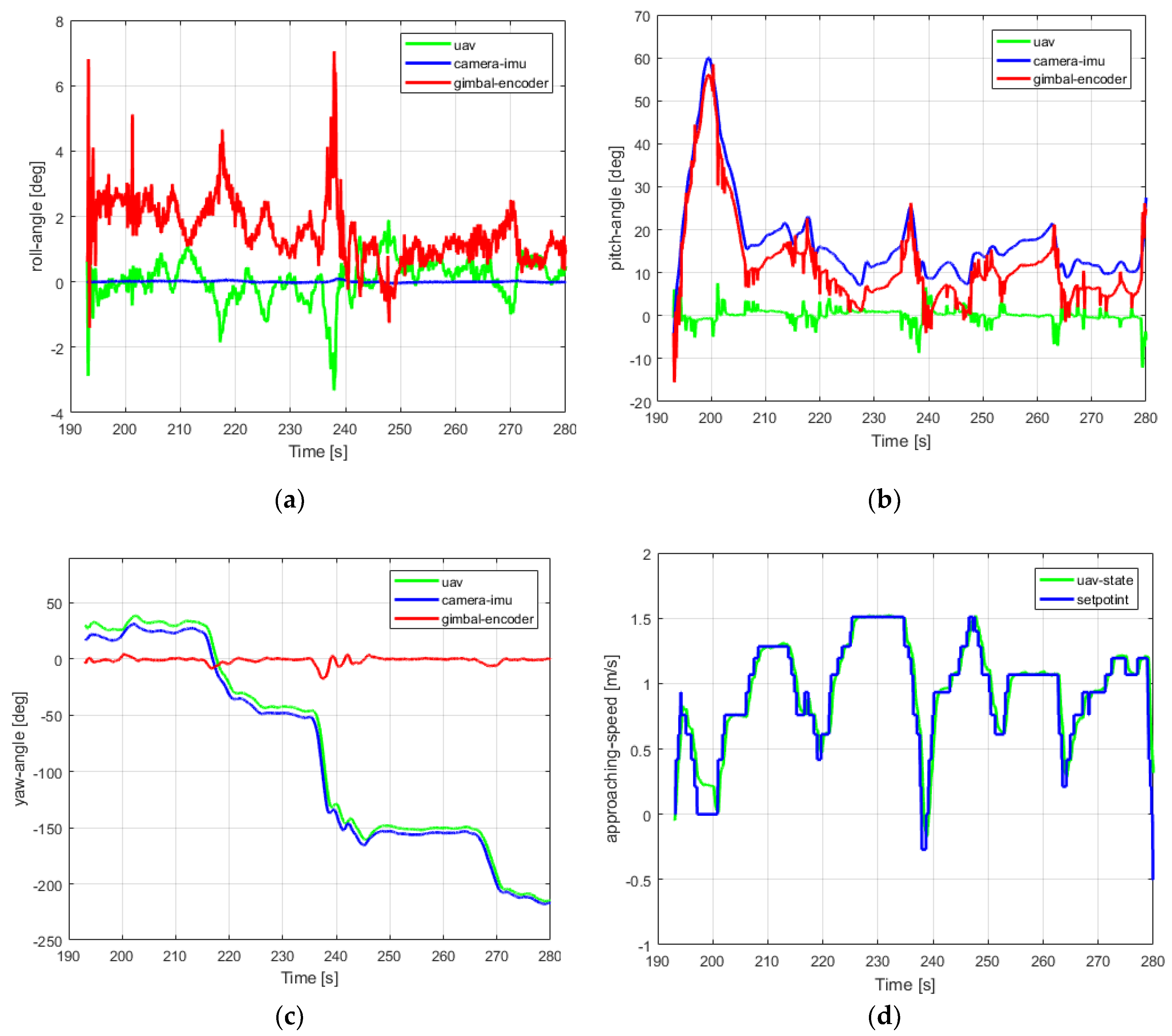
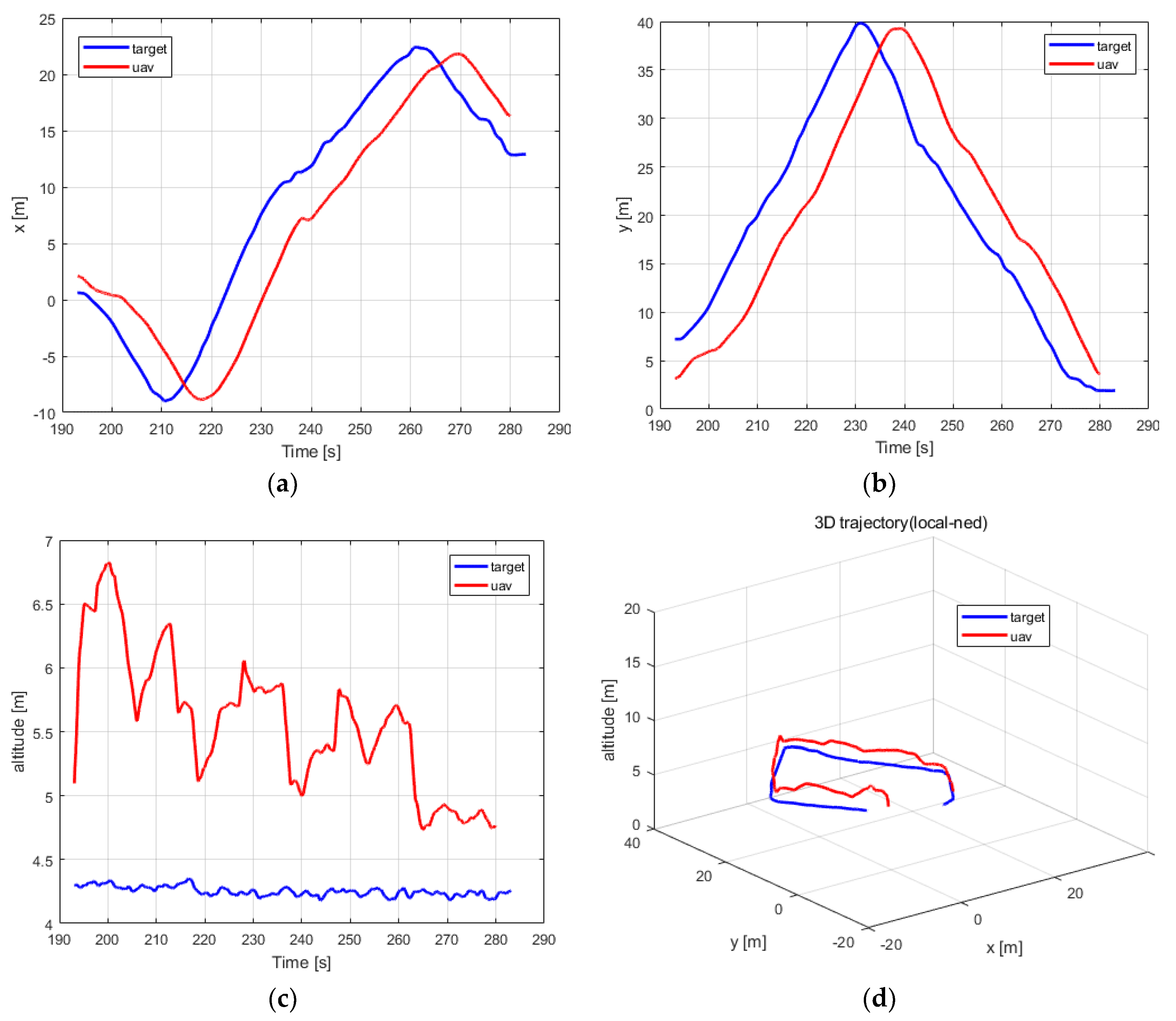
5.2. Experimental Results and Analysis
6. Conclusions
Supplementary Materials
Author Contributions
Funding
Acknowledgments
Conflicts of Interest
References
- Cai, G.; Dias, J.; Seneviratne, L. A Survey of Small-Scale Unmanned Aerial Vehicles: Recent Advances and Future Development Trends. Unmanned Syst. 2014, 2, 175–199. [Google Scholar] [CrossRef]
- Tomic, T.; Schmid, K.; Lutz, P.; Domel, A.; Kassecker, M.; Mair, E.; Grixa, I.L.; Ruess, F.; Suppa, M.; Burschka, D. Toward a Fully Autonomous UAV: Research Platform for Indoor and Outdoor Urban Search and Rescue. Robot. Autom. Mag. 2012, 19, 46–56. [Google Scholar] [CrossRef]
- Judy, J.W. Microelectromechanical systems (MEMS): Fabrication, design and applications. Smart Mater. Struct. 2001, 10, 1115–1134. [Google Scholar] [CrossRef]
- Zhao, Z.; Yang, J.; Niu, Y.; Zhang, Y.; Shen, L. A Hierarchical Cooperative Mission Planning Mechanism for Multiple Unmanned Aerial Vehicles. Electronics 2019, 8, 443. [Google Scholar] [CrossRef]
- Laliberte, A.S.; Jeffrey, E.H.; Rango, A.; Winters, C. Acquisition, Orthorectification, and Object-based Classification of Unmanned Aerial Vehicle (UAV) Imagery for Rangeland Monitoring. Photogramm. Eng. Remote Sens. 2015, 76, 661–672. [Google Scholar] [CrossRef]
- Hausamann, D.; Zirnig, W.; Schreier, G.; Strobl, P. Monitoring of gas pipelines - a civil UAV application. Aircr. Eng. Aerosp. Technol. 2005, 77, 352–360. [Google Scholar] [CrossRef]
- Bristeau, P.J.; Callou, F.; Vissière, D.; Petit, N. The Navigation and Control technology inside the AR.Drone micro UAV. In Proceedings of the 18th World Congress of the International Federation of Automatic Control (IFAC), Milano, Italy, 28 August–2 September 2011; pp. 1477–1484. [Google Scholar]
- Tai, J.C.; Tseng, S.T.; Lin, C.P.; Song, K.T. Real-time image tracking for automatic traffic monitoring and enforcement applications. Image Vis. Comput. 2004, 22, 485–501. [Google Scholar] [CrossRef]
- Chow, J.Y.J. Dynamic UAV-based traffic monitoring under uncertainty as a stochastic arc-inventory routing policy. Int. J. Transp. Sci. Technol. 2016, 5, 167–185. [Google Scholar] [CrossRef]
- Silvagni, M.; Tonoli, A.; Zenerino, E.; Chiaberge, M. Multipurpose UAV for search and rescue operations in mountain avalanche events. Geomat. Nat. Hazards Risk 2017, 8, 18–33. [Google Scholar] [CrossRef]
- Bejiga, M.B.; Zeggada, A.; Nouffidj, A.; Melgani, F. A Convolutional Neural Network Approach for Assisting Avalanche Search and Rescue Operations with UAV Imagery. Remote Sens. 2017, 9, 100. [Google Scholar] [CrossRef]
- Li, Z.; Liu, Y.; Walker, R.; Hayward, R.; Zhang, J. Towards automatic power line detection for a UAV surveillance system using pulse coupled neural filter and an improved Hough transform. Mach. Vis. Appl. 2010, 21, 677–686. [Google Scholar] [CrossRef]
- Sa, I.; Hrabar, S.; Corke, P. Inspection of Pole-Like Structures Using a Visual-Inertial Aided VTOL Platform with Shared Autonomy. Sensors 2015, 15, 22003–22048. [Google Scholar] [CrossRef] [PubMed]
- Chuang, H.-M.; He, D.; Namiki, A. Autonomous Target Tracking of UAV Using High-Speed Visual Feedback. Appl. Sci. 2019, 9, 4552. [Google Scholar] [CrossRef]
- Wang, F.; Cong, X.-B.; Shi, C.-G.; Sellathurai, M. Target Tracking While Jamming by Airborne Radar for Low Probability of Detection. Sensors 2018, 18, 2903. [Google Scholar] [CrossRef] [PubMed]
- Wang, Y.; Lei, H.; Ye, J.; Bu, X. Backstepping Sliding Mode Control for Radar Seeker Servo System Considering Guidance and Control System. Sensors 2018, 18, 2927. [Google Scholar] [CrossRef]
- Liu, X.; Zhang, S.; Tian, J.; Liu, L. An Onboard Vision-Based System for Autonomous Landing of a Low-Cost Quadrotor on a Novel Landing Pad. Sensors 2019, 19, 4703. [Google Scholar] [CrossRef]
- Yang, S.; Scherer, S.A.; Schauwecker, K.; Zell, A. Autonomous Landing of MAVs on an Arbitrarily Textured Landing Site Using Onboard Monocular Vision. J. Intell. Robot. Syst. 2014, 74, 27–43. [Google Scholar] [CrossRef]
- Wenzel, K.E.; Rosset, P.; Zell, A. Low-cost visual tracking of a landing place and hovering flight control with a microcontroller. J. Intell. Robot. Syst. 2010, 57, 297–311. [Google Scholar] [CrossRef]
- Saripalli, S.; Montgomery, J.F.; Sukhatme, G.S. Visually guided landing of an unmanned aerial vehicle. IEEE Trans. Robot. Autom. 2003, 19, 371–380. [Google Scholar] [CrossRef]
- Yang, S.; Scherer, S.A.; Zell, A. An onboard monocular vision system for autonomous takeoff, hovering and landing of a micro aerial vehicle. J. Intell. Robot. Syst. 2013, 69, 499–515. [Google Scholar] [CrossRef]
- Olson, E. AprilTag: A robust and flexible visual fiducial system. In Proceedings of the IEEE International Conference on Robotics and Automation (ICRA), Shanghai, China, 9–13 May 2011; pp. 3400–3407. [Google Scholar]
- Garrido-Jurado, S.; Muñoz-Salinas, R.; Madrid-Cuevas, F.J.; Marín-Jiménez, M.J. Automatic generation and detection of highly reliable fiducial markers under occlusion. Pattern Recognit. 2014, 47, 2280–2292. [Google Scholar] [CrossRef]
- Kyristsis, S.; Antonopoulos, A.; Chanialakis, T.; Stefanakis, E.; Linardos, C.; Tripolitsiotis, A.; Partsinevelos, P. Towards Autonomous Modular UAV Missions: The Detection, Geo-Location and Landing Paradigm. Sensors 2016, 16, 1844. [Google Scholar] [CrossRef] [PubMed]
- Pestana, J.; Sanchez-Lopez, J.L.; de la Puente, P.; Carrio, A.; Campoy, P. A Vision-based Quadrotor Swarm for the participation in the 2013 International Micro Air Vehicle Competition. In Proceedings of the 2014 International Conference on Unmanned Aircraft Systems (ICUAS), Orlando, FL, USA, 27–30 May 2014; pp. 617–622. [Google Scholar]
- Ma, L.; Hovakimyan, N. Vision-based cyclic pursuit for cooperative target tracking. In Proceedings of the 2011 American Control Conference, San Francisco, CA, USA, 29 June–1 July 2011; pp. 4616–4621. [Google Scholar]
- Ross, D.A.; Lim, J.; Lin, R.S.; Yang, M.H. Incremental Learning for Robust Visual Tracking. Int. J. Comput. Vis. 2008, 77, 125–141. [Google Scholar] [CrossRef]
- Mei, X.; Ling, H. Robust visual tracking using ℓ1 minimization. In Proceedings of the IEEE International Conference on Computer Vision (ICCV), Kyoto, Japan, 29 September–2 October 2009; pp. 1436–1443. [Google Scholar]
- Li, H.; Shen, C.; Shi, Q. Real-time visual tracking using compressive sensing. In Proceedings of the 24th IEEE Conference on Computer Vision and Pattern Recognition (CVPR), Colorado Springs, CO, USA, 20–25 June 2011; pp. 1305–1312. [Google Scholar]
- Wang, S.; Lu, H.; Yang, F.; Yang, M.H. Superpixel tracking. In Proceedings of the IEEE International Conference on Computer Vision (ICCV), Barcelona, Spain, 6–13 November 2011; pp. 1323–1330. [Google Scholar]
- Cheng, Y. Mean Shift, Mode Seeking, and Clustering. IEEE Trans. Pattern Anal. Mach. Intell. 1995, 17, 790–799. [Google Scholar] [CrossRef]
- Comaniciu, D.; Meer, P. Mean Shift: A Robust Approach Toward Feature Space Analysis. IEEE Trans. Pattern Anal. Mach. Intell. 2002, 24, 603–619. [Google Scholar] [CrossRef]
- Collins, R.T. Mean-shift blob tracking through scale space. In Proceedings of the IEEE Computer Society Conference on Computer Vision and Pattern Recognition (CVPR), Madison, WI, USA, 16–22 June 2003; pp. 234–240. [Google Scholar]
- Bradski, G.R. Computer Vision Face Tracking for Use in a Perceptual User Interface. Intel Technol. J. 1998, 2, 12–21. [Google Scholar]
- Babenko, B.; Yang, M.H.; Belongie, S. Robust Object Tracking with Online Multiple Instance Learning. IEEE Trans. Pattern Anal. Mach. Intell. 2011, 33, 1619–1632. [Google Scholar] [CrossRef]
- Hare, S.; Golodetz, S.; Saffari, A.; Vineet, V.; Cheng, M.M.; Hicks, S.L.; Torr, P.H. Struck: Structured Output Tracking with Kernels. IEEE Trans. Pattern Anal. Mach. Intell. 2016, 38, 2096–2109. [Google Scholar] [CrossRef]
- Grabner, H.; Bischof, H. Online Boosting and Vision. In Proceedings of the IEEE Computer Society Conference on Computer Vision and Pattern Recognition (CVPR), New York, NY, USA, 17–22 June 2006; pp. 260–267. [Google Scholar]
- Kalal, Z.; Mikolajczyk, K.; Matas, J. Tracking-Learning-Detection. IEEE Trans. Softw. Eng. 2011, 34, 1409–1422. [Google Scholar] [CrossRef]
- Wei, J.; Liu, F. Coupled-Region Visual Tracking Formulation Based on a Discriminative Correlation Filter Bank. Electronics 2018, 7, 244. [Google Scholar] [CrossRef]
- Bolme, D.S.; Beveridge, J.R.; Draper, B.A.; Lui, Y.M. Visual object tracking using adaptive correlation filters. In Proceedings of the IEEE Computer Society Conference on Computer Vision and Pattern Recognition (CVPR), San Francisco, FL, USA, 13–18 June 2010; pp. 2544–2550. [Google Scholar]
- Henriques, J.F.; Caseiro, R.; Martins, P.; Batista, J. Exploiting the Circulant Structure of Tracking-by-Detection with Kernels. In Proceedings of the 12th European conference on Computer Vision, Florence, Italy, 7–13 October 2012; Springer: Berlin, Germany, 2012; pp. 702–715. [Google Scholar]
- Henriques, J.F.; Caseiro, R.; Martins, P.; Batista, J. High-Speed Tracking with Kernelized Correlation Filters. IEEE Trans. Pattern Anal. Mach. Intell. 2015, 37, 583–596. [Google Scholar] [CrossRef] [PubMed]
- Wu, Y.; Lim, J.; Yang, M.H. Online Object Tracking: A Benchmark. In Proceedings of the Computer Vision and Pattern Recognition (CVPR), Portland, OR, USA, 23–28 June 2013; pp. 2411–2418. [Google Scholar]
- Montero, A.S.; Lang, J.; Laganière, R. Scalable Kernel Correlation Filter with Sparse Feature Integration. In Proceedings of the IEEE International Conference on Computer Vision Workshop, Santiago, Chile, 7–13 December 2015; pp. 587–594. [Google Scholar]
- Zhang, Y.H.; Zeng, C.N.; Liang, H.; Luo, J.; Xu, F. A visual target tracking algorithm based on improved Kernelized Correlation Filters. Proceedings of 2016 IEEE International Conference on Mechatronics and Automation, Harbin, China, 7–10 August 2016; pp. 199–204. [Google Scholar]
- Santos, D.A.; Gonçalves, P.F.S.M. Attitude Determination of Multirotor Aerial Vehicles Using Camera Vector Measurements. J. Intell. Robot. Syst. 2016, 86, 1–11. [Google Scholar] [CrossRef]
- Falanga, D.; Zanchettin, A.; Simovic, A.; Delmerico, J.; Scaramuzza, D. Vision-based Autonomous Quadrotor Landing on a Moving Platform. In Proceedings of the 15th IEEE International Symposium on Safety, Security, and Rescue Robotics (SSRR), Shanghai, China, 11–13 October 2017. [Google Scholar]
- Borowczyk, A.; Nguyen, D.T.; Phu-Van Nguyen, A.; Nguyen, D.Q.; Saussié, D.; Le Ny, J. Autonomous Landing of a Multirotor Micro Air Vehicle on a High Velocity Ground Vehicle. arXiv 2016, arXiv:1611.07329. Available online: http://arxiv.org/abs/1611.07329 (accessed on 26 May 2020).
- Quigley, M.; Goodrich, M.A.; Griffiths, S.; Eldredge, A.; Beard, R.W. Target Acquisition, Localization, and Surveillance Using a Fixed-Wing Mini-UAV and Gimbaled Camera. In Proceedings of the 2005 IEEE International Conference on Robotics and Automation, Barcelona, Spain, 18–22 April 2005; pp. 2600–2605. [Google Scholar]
- Jakobsen, O.C.; Johnson, E. Control Architecture for a UAV-Mounted Pan/Tilt/Roll Camera Gimbal. In Proceedings of the Infotech@Aerospace, AIAA 2005, Arlington, VA, USA, 26–29 September 2005; p. 7145. [Google Scholar]
- Whitacre, W.; Campbell, M.; Wheeler, M.; Stevenson, D. Flight Results from Tracking Ground Targets Using SeaScan UAVs with Gimballing Cameras. In Proceedings of the 2007 American Control Conference, New York, NY, USA, 11–13 July 2007; pp. 377–383. [Google Scholar]
- Dobrokhodov, V.N.; Kaminer, I.I.; Jones, K.D.; Ghabcheloo, R. Vision-based tracking and motion estimation for moving targets using small UAVs. In Proceedings of the 2006 American Control Conference, Minneapolis, MN, USA, 14–16 June 2006. [Google Scholar]
- Johansson, J. Modelling and Control of an Advanced Camera Gimbal. Teknik Och Teknologier, 2012. Available online: http://www.diva-portal.org/smash/get/diva2:575341/FULLTEXT01.pdf (accessed on 26 May 2020).
- Kazemy, A.; Siahi, M. Equations of Motion Extraction for a Three Axes Gimbal System. Modares J. Electr. Eng. 2014, 13, 37–43. [Google Scholar]
- Barnes, F.N. Stable Member Equations of Motion for a Three-Axis Gyro Stabilized Platform. IEEE Trans. Aerosp. Electron. Syst. 1971, 7, 830–842. [Google Scholar] [CrossRef]
- Otlowski, D.R.; Wiener, K.; Rathbun, B.A. Mass properties factors in achieving stable imagery from a gimbal mounted camera. In Airborne Intelligence, Surveillance, Reconnaissance (ISR) Systems and Applications 2008; International Society for Optics and Photonics: Orlando, FL, USA, 2008; Volume 6946. [Google Scholar]
- Rifkin, R.; Yeo, G.; Poggio, T. Regularized Least-Squares Classification. In Nato Science Series Sub Series III Computer and Systems Sciences; IOS Press: Amsterdam, The Netherlands, 2003; Volume 190, pp. 131–154. [Google Scholar]
- Islam, M.M.; Hu, G.; Liu, Q. Online Model Updating and Dynamic Learning Rate-Based Robust Object Tracking. Sensors 2018, 18, 2046. [Google Scholar] [CrossRef]
- Pestana, J.; Mellado-Bataller, I.; Sanchez-Lopez, J.L.; Fu, C.; Mondragon, I.F.; Campoy, P. A General Purpose Configurable Controller for Indoors and Outdoors GPS-Denied Navigation for Multirotor Unmanned Aerial Vehicles. J. Intell. Robot. Syst. 2014, 73, 387–400. [Google Scholar] [CrossRef]
- Tan, R.; Kumar, M. Tracking of Ground Mobile Targets by Quadrotor Unmanned Aerial Vehicles. Unmanned Syst. 2014, 2, 157–173. [Google Scholar] [CrossRef]
- Guelman, M. The Closed-Form Solution of True Proportional Navigation. IEEE Trans. Aerosp. Electron. Syst. 1976, 12, 472–482. [Google Scholar] [CrossRef]
- Yuan, P.J.; Chern, J.S. Ideal proportional navigation. Adv. Astronaut. Sci. 1992, 95, 81374. [Google Scholar] [CrossRef]
- Mahapatra, P.R.; Shukla, U.S. Accurate solution of proportional navigation for maneuvering targets. IEEE Trans. Aerosp. Electron. Syst. 1989, 25, 81–89. [Google Scholar] [CrossRef][Green Version]
- Park, S.; Deyst, J.; How, J. A new nonlinear guidance logic for trajectory tracking. In Proceedings of the AIAA Guidance, Navigation, and Control Conference and Exhibit, Providence, RI, USA, 16–19 August 2004. [Google Scholar]
- Mathisen, S.H.; Gryte, K.; Johansen, T.; Fossen, T.I. Non-linear Model Predictive Control for Longitudinal and Lateral Guidance of a Small Fixed-Wing UAV in Precision Deep Stall Landing. In Proceedings of the AIAA SciTech, San Diego, CA, USA, 4–8 January 2016. [Google Scholar]
- Pixhawk. Available online: https://pixhawk.org/ (accessed on 20 May 2020).
- Mavros. Available online: https://github.com/mavlink/mavros/ (accessed on 20 May 2020).
- Ros. Available online: http://www.ros.org/ (accessed on 20 May 2020).
- Mathisen, S.H.; Gryte, K.; Johansen, T.; Fossen, T.I. Cross-Correlation-Based Structural System Identification Using Unmanned Aerial Vehicles. Sensors 2017, 17, 2075. [Google Scholar]


| RMSE (Pixel) | Azimuth | Elevation | 2D |
|---|---|---|---|
| Step test | 31.57 | 4.83 | 31.94 |
| Pedestrian following | 9.34 | 5.07 | 10.63 |
| Drone tracking | 21.50 | 19.28 | 28.88 |
© 2020 by the authors. Licensee MDPI, Basel, Switzerland. This article is an open access article distributed under the terms and conditions of the Creative Commons Attribution (CC BY) license (http://creativecommons.org/licenses/by/4.0/).
Share and Cite
Liu, X.; Yang, Y.; Ma, C.; Li, J.; Zhang, S. Real-Time Visual Tracking of Moving Targets Using a Low-Cost Unmanned Aerial Vehicle with a 3-Axis Stabilized Gimbal System. Appl. Sci. 2020, 10, 5064. https://doi.org/10.3390/app10155064
Liu X, Yang Y, Ma C, Li J, Zhang S. Real-Time Visual Tracking of Moving Targets Using a Low-Cost Unmanned Aerial Vehicle with a 3-Axis Stabilized Gimbal System. Applied Sciences. 2020; 10(15):5064. https://doi.org/10.3390/app10155064
Chicago/Turabian StyleLiu, Xuancen, Yueneng Yang, Chenxiang Ma, Jie Li, and Shifeng Zhang. 2020. "Real-Time Visual Tracking of Moving Targets Using a Low-Cost Unmanned Aerial Vehicle with a 3-Axis Stabilized Gimbal System" Applied Sciences 10, no. 15: 5064. https://doi.org/10.3390/app10155064
APA StyleLiu, X., Yang, Y., Ma, C., Li, J., & Zhang, S. (2020). Real-Time Visual Tracking of Moving Targets Using a Low-Cost Unmanned Aerial Vehicle with a 3-Axis Stabilized Gimbal System. Applied Sciences, 10(15), 5064. https://doi.org/10.3390/app10155064