Abstract
Electrophoresis allows us to identify the types of proteins present in food, DNA, tissues and more. With the help of the molecular marker their weight is known, these markers are applied within the one-dimensional gel, and their protein value is known by means of marks. In this research, the molecular marker is obtained and the wavelet transform (WT) is obtained, generating approximation coefficients, which were taken to determine a molecular weight using three classification paradigms. The first paradigm is an approach in content-based image retrieval (CBIR) which makes a detection of the molecular weight in electrophoresis samples. The second approach is a neural network, thus two models are employed: self-organization maps (SOM) and back propagation in a supervised and unsupervised way, respectively. The third approach is based in a J48 decision tree. A comparison is made between the three paradigms for molecular weight computation. Neural networks obtained an improvement in the precision compared versus the CBIR-WT. Five parametric statistics were generated from the wavelet approximation coefficients. The CBIR-WT, SOM, back propagation and J48 were decisive for the classification and calculation of the molecular weight of each protein stain in the one-dimensional electrophoresis gel.
1. Introduction
There is a analytical approach called electrophoresis which is used for chemistry professionals through an electric field. The objective of this field is the separation of proteins. The substances used in this task are silver or blue coomassie. Then, a generation of the sodium dodecyl sulphate polyacrylamide gel electrophoresis (SDS-PAGE) is achieved. Then, channels of samples can be placed in the SDS-PAGE lane. Then, the proteins can be put in the bottom of the lane in the function of its molecular weight. Then, an electric field is applied and the opposition of the molecules can be observed. A relativizing substance is placed and allows the visualization of protein molecules in the gel. This previous explanation is about the electrophoresis process [1]. Thus, this research problem lies in that the molecular way can be measured from images of the lanes.
On the other hand, the digital image processing area has the objective of recognizing, analyzing, and improving images to emulate the behavior of the human eye. The process takes an image and processes it by means of two directions: x and y, likewise a function. Each of the pixels is the meaning of a gray level. There are several processes that can be done in an image: filtering, quality improvement, recognition, classification, segmentation, brightening, or labeling [2].
The state of the art that has been carried out shows us only a few works that measure the molecular weights of proteins. The works in the area have focused on improving the images of the electrophoresis plates, filtering, contrast, lighting, and brightness. However, in most of them, there is no measurement by intelligent paradigms. The electrophoresis samples are taken from tissues, food, and medications, among others. On the other hand, the types of samples are of different dimensions, they can be in 1D or 2D. They have also included work that, although they do not deal with electrophoresis samples, do show some classification work with the intelligent paradigms proposed here for the measurement of molecular weights.
The purpose of this research is to make a measurement of molecular weight in protein samples, not only quantitatively, but also visually. That is, calculating the molecular weight in kilodaltons (kD) and at the same time providing the industrial chemistry expert with other images of similar samples containing the same molecular weight by means of retrieval of visual information.
The motivation for this work is the need for experts in industrial chemistry to perform molecular weight measurements by more accurate and economic means. These measurements are intended to be associated increasingly fast, if possible, with other similar measurements for subsequent analysis for various activities and statistics specific to the expert such as histories, visual associations, comparisons of different protein origins, and so forth.
It is important to mention that also, within the state of the art, there is no work that makes protein measurements visually and there is rarely work on molecular weight measurements numerically speaking. The work or investigations that currently exist consist of the analysis or processing of the samples, but they do not attack or resolve the calculation or measurement of molecular weights as such.
The hypothesis of this work is to perform a molecular weight measurement of protein profile electrophoresis samples using four different intelligent paradigms. These paradigms contemplate systems based on two different artificial neural networks, one decision tree method, and one content-based retrieval system. It is also intended that from electrophoresis images, the approximation coefficients can be obtained by means of wavelet transforms. Wavelet transforms allow obtaining parametric statistics of the samples that finally define certain ranges of values that allow mapping to molecular weights in kilodaltons.
2. State of Art in Electrophoresis and Image Retrieval
The work of [3] works with two-dimensional electrophoresis samples and uses mass spectrography for proteoforms detection. Several spots of proteins can be found in each 2D gel. Then, the electric field is applied and the identification of proteins can be achieved.
There are commercial options that perform the electrophoresis measurement. In the comparative analysis carried out by [4], the studies carried out on Total Lab 120 and Lab Image 1D are shown. These options show different functions, among them the molecular weight measurements and the improvement of the electrophoresis samples for analysis. In this study, it is possible to show that the measurements and improvements in the samples vary depending on the software used.
Another system that is performed for the measurement of molecular weights also uses wavelet transform. In the work done by [5], three wavelet transforms are implemented: Daubechies level 8 with decomposition 15 (DB8-15), biorthogonal level 4.4 with decomposition 7 (BIOR4.4-7), and biorthogonal 3.3 with decomposition 4 (BIOR3.3-4). A reliability of 95% is obtained in the results. The application is in the fibromyalgia detection, providing the ability to provide medication for its treatment to those patients who require it.
Another type of application for measuring molecular weights is given in the capillary analysis, where protein detection is important for patients suffering from alopecia or who may be undergoing chemotherapy treatments. The work is carried out by means of cellular analysis with mass spectrometry [6].
The work carried out by [7] exposes an analysis and improvement of images of electrophoresis samples. The research focuses on the improvement of brightness, contrast, and identification of protein spots. Even spots that are imperceptible to the human eye are detected. Only a maximum and minimum algorithm is used but a molecular weight measurement is not performed.
Another way to obtain similarity in the images is that in [8] proposed an algorithm that improves distinctive characters of the image using spatial distribution, which is calculated by means of the location histogram. The location histogram provides scales and orientations of the local characteristics, in order to achieve a good recovery.
Working with the analysis of images in myocardium samples provides quantitative data. Using machine vision, in this work they can classify the results and even achieve a prediction, for example, with artificial neural networks (ANN) (see [9]) and decision trees.
A job where only decision trees were applied was done in [10], where they obtained a 78.39% accuracy in the classification, their objective was to use a decision tree to analyze the data and to establish a combination and to obtain a classification, the whole process started occupying 10 input variables.
In [11], they made a model based on decision trees and ANN, they applied the Chi-Square Automatic Interaction Detection (CHAID) model with which they took six characteristics and obtained 74.2% effectiveness, generating four groups of classification, specifies that two of those four are main. When applying the neural network, they increased four characteristics, having 10 as the input to the ANN and obtained 75% effectiveness.
A similar process is done by [12], where they trained neural networks and applied a genetic algorithm (GA) to select the weights of the networks. From the GA they selected 84 ANNs that generated 70% precision, with these ANNs they formed a multi-agent system which obtained an accuracy between 72% and 76.6%, but it is mentioned that these output results must be corroborated at a later stage.
The work of models in multi objective optimization using an artificial neural network (ANN) and adaptive neuro-fuzzy inference system (ANFIS) with which they seek to predict the results, the ANN model they used was feed forward backward propagation. They observed that placing the neural network as a fitness function in a genetic algorithm (GA) obtained better results than with an ANFIS because the ANN uses experimental data points towards more effective learning to predict the results (see [13]).
To make a more precise analysis of the differences, contributions, objectives pursued, and intelligent methods used in the area, Table 1 is shown, where the first column mentions the technique applied. The second column mentions the kind of data used. The third column explains the main objective of the related work. The fourth column points out the author of the corresponding research.

Table 1.
Comparative table of related works in electrophoresis and/or diverse paradigms.
In this table, we can see that the state of the art can be divided into three modalities: (a) work that analyzes samples of electrophoresis for their improvement and detection of molecules, (b) work that performs molecular weight measurements, and (c) work that implements intelligent paradigms applied to diagnostics or data analysis.
We can summarize then that in the state of the art, four works focus on the group, that is, on the analysis and improvement of electrophoresis images. It is also shown that four works focus on the application of intelligent paradigms in image diagnosis or analysis. However, only two of them [4,5,6] are dedicated to the improvement of images and the measurement of molecular weights by means of intelligent techniques such as the use of the wavelet transform, but they do not perform a recovery based on visual information, as in the proposal of this research.
More specifically, from the three strongest related works we can say specifically that:
- In Kahlenberg’s 2012 paper [4], a molecular weight measurement is performed, but it is highlighted that there are calculation irregularities depending on commercial versions of the compared software.
- In the case of Reza and Shorabi of 2018 [5], a molecular weight detection with 95% accuracy is performed using also wavelet transform but with different families or levels.
- In the work of Zhou of 2019 [6], a cell detection in electrophoresis is done by means of digital image processing, without making a sample recovery or a molecular weight measure.
Our main contribution lies in providing image analysis with wavelet transforms, the novel contribution lies in a visual retrieval system of query images and a 96.7% in molecular weight detection unlike the 95% of Reza and Shorabi. Our proposal is a free system unlike the commercial Total Lab and Lab Image software analyzed by Kahlenberg [4]. Even though other work has been done with wavelet retrieval, the percentage is surpassed, and the content-based retrieval system in electrophoresis images is not provided in other works so far.
In the case of the work previously carried out by the same authors of this research published in [14], it should be noted that only a visual recovery system with a 93% recovery was carried out. In this new research proposal, four intelligent molecular weight measurement paradigms are implemented and compared between them, improving the measurement percentage in 96.7% through a back propagation neural network.
3. Molecular Weight Measurement System Using Intelligent Classification in One-Dimensional Sample Electrophoresis
This work carries out an application of intelligent classification paradigms, the first is by means of the wavelet transform, obtaining the approximation coefficients and generating five parametric statistics with which the input variables will be, in the first case, using the Euclidean metric and generating the matrix and classifying the molecular weight of the samples through four ranges based solely on their minimum value. In the ANN application, we take two types, back propagation and self-organization maps (SOM) where five approximation values are provided as input, in the same way as in the decision tree using algorithm J48.
This research work is divided into three phases (See Figure 1), the first phase focuses on the creation and obtainment of electrophoresis samples, starting from a chemical process in the electrophoresis chamber to generate the polyacrylamide gel. Each gel contains 10 lanes, these lanes are scanned and each process contains protein information. Once the gel is scanned, each lane is separated. The RGB color map is used. From it, the gray levels are obtained. The second phase of the investigation consists of the application of the wavelet transform in the daubechies variant, decomposing the image of each sample up to level 3. This phase contains two interfaces, the first to load an electrophoresis sample and present its visual information: the minimum, maximum, mean, median, and standard deviation values. These values are obtained using the approximation coefficients, likewise, the detected molecular weight is presented. The second interface retrieves the five electrophoresis samples that have the most similarity to the query sample in the first interface. In the third phase we apply classification paradigms, with the four detection of molecular weight groups generated, the first paradigm is a CBIR system that uses a Euclidean distance to generate a matrix, followed by ordering and searching for the five similar values of molecular weights. The second paradigm is the neural networks, where five input data are fed to it, and four classification groups, as well as the decision tree.
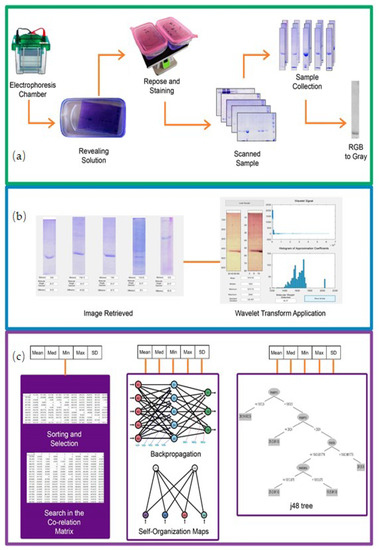
Figure 1.
Diagram of the system, divided into three phases: First phase (in green square) is about electrophoresis process. Second phase (in blue square) is about feature extraction with wavelet transform. Third phase (in purple square) is about the three intelligent paradigms tested: (a) Content Based Image retrieval System, (b) Neural Networks (Backpropagation and Self Organization Maps) and (c) J48 Decision Tree.
To determine the classification groups, we know the operation of a molecular marker, four classification groups were defined to determine the molecular weight of the sample. For the CBIR-WT model, we observed that only the minimum value of each sample helps to classify and calculate the weight, for the back propagation, SOM, and J48, the five characteristics previously obtained were used.
The four groups are classified as follows, taking the minimum value as the main characteristic.
Thus, it is clear that the second interface inside the system allows us to classify the electrophoresis samples from our database and we are able to recover similar samples with a similar molecular weight.
4. Materials and Methods
In this section the foundations of this research are explained. The first basic concept is electrophoresis, a process of industrial chemistry that creates the samples and is the source of inspiration for the measurement of molecular weights in proteins. The second basic concept is the wavelet transform. The wavelet transform is widely used in the area of visual information retrieval, since it is an effective method to extract the characteristics of a two-dimensional signal. The characteristics in time and frequency are detectable from this type of transformation.
The third concept is the CBIR, this approach helps to carry out the investigation trough the Euclidean distance. The fourth concept is the neural networks in the self-organization maps and back propagation algorithm which describes how they work and exposes the differences in classifications. Finally, we have the concept of decision trees, where we detail how they work and how they make the classification for molecular weight measurement.
4.1. Electrophoresis
Electrophoresis is an analytical technique used by professionals in the area of industrial chemistry to obtain protein profiles and the analysis of proteins. Its objective is to separate the proteins by means of an electric field in a chamber device (see Figure 2). This technique is carried out in poliyacrylamide gel (PAGE), in which the protein samples are placed and then, the electric field is applied. Sodium dodecylsulfate (SDS) is also used in the natural charge of the proteins, so they can be computed and separated on the basis of their mass. Therefore, SDS-PAGE electrophoresis evaluates the purity and estimates the atomic weight of the proteins [1].
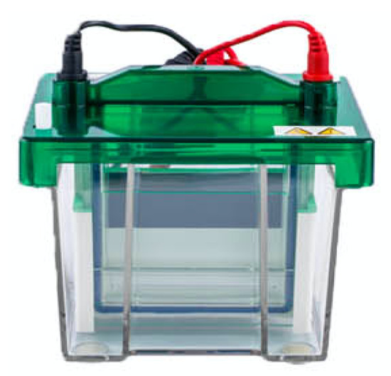
Figure 2.
Electrophoresis chamber.
The electrophoresis process begins with the placement of the samples in each lane of the gel. Then, the gel is poured into the electrophoresis chamber, which allows the migration of the proteins. The speed of migration of the proteins is proportional to the percentage of the pore of the material and its mass, those that are of greater weight, show resistance, and migrate slowly. Those with less weight are those that end up until the end of it, meaning that they will migrate faster.
The analysis of electrophoresis uses a standard of measurement of molecular weights, called a marker, its value is around $300 US, and its function is precisely to measure the molecular weight of the proteins in question, or the sample in turn. The weight is measured in kilodaltons (kD). There are different types of markers, the standard is two colors, the standard of five colors that belong to the standards of the brand kaleidoscope, where the ranges of the markers vary between 10–250 kD. In commercial markers, the colors indicate the range and type of protein contained in the electrophoresis analysis.
4.2. Wavelet Transform
The wavelet transform works with audio signals and images, that is, with one-dimensional or two-dimensional signals. Its function is to decompose the signal into various components, with this, it is possible to locate the approximation coefficients and the detail coefficients of the image. The process starts with the original image and then decomposes the image into sub-images until it reaches a low-resolution image. The family of wavelet transform used in this work is the Daubechies transform that was proposed by Ingrid Daubechies, as defined in [15]. This type of wavelet was chosen, due to its effectiveness to highlight the coefficients of detail of the type of electrophoresis samples.
Then, a Daubechies transform Type 1 at decomposition level 3 is mapped as where draws the approximation coefficients and extracts the detail coefficients. Each value of the signals composed by the coefficients, is formed by a scalar product, being for the approximation matrix , and for the detail matrix . Where is the scaled entry signal at level 3, and is the wavelet transform at level 3. The input signal is taken as indicated in the Equation (1).
If is the input image, then, Equation (2) represents the calculation of the approximation coefficients.
where, is redefined with the substitution of as
For the decomposition matrix computation, Equation (4) represents the computation of detail coefficients.
where, values, can be defined likewise , and Equation (4) can be redefined as:
The wavelet transforms, in any of its variants, can generate several levels of sub-signals, once the first level is obtained, the same calculations are made, sub signal by sub signal. More information regarding this type of transform can be found in [15,16].
The Wavelet Daubechies Transform Type 1 is chosen in decomposition at level 1, and is selected because its coefficients obtain a minimum that adapts to the ranges required for the measurement of molecular weights.
4.3. Contend Based Image Retrieval
The Content Based Image Retrieval (CBIR) systems allow us, as the name implies, to retrieve images through the content of the input image, these systems help various professional areas such as medicine, biology, web searches, education, among others [17]. CBIR systems help make the recovery of visual information possible and they focus on image characteristics such as texture, color, shape, or intensity.
A typical image recovery system should contain the query image and the images in the database that will help to extract the characteristics to find the similarity between them (see Figure 3).
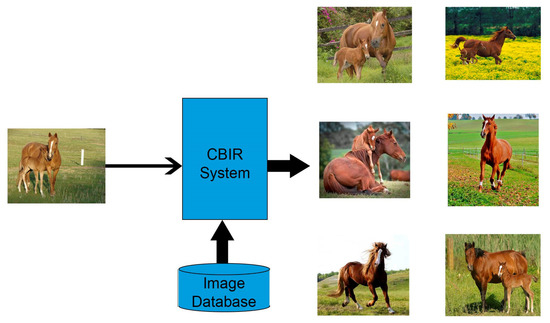
Figure 3.
CBIR system which starts with an input image and this feature was taken out to obtain a guide to retrieve the images with greater similarity or meet all or most of the characteristics of the input image (taken from [17]).
4.4. Euclidean Metric
This metric is also known as the Euclidean distance, with which the search of the shortest distance between two points is calculated using the Pythagorean Theorem.
For pixels , and z, with coordinates (), (), and (), respectively, D is a distance function or metric if:
- ,
- and
4.5. Recall and Presicion
Recall and precision are used to evaluate information retrieval systems where you have R as the set of number of images, a response set A, images at the intersection of the set R, and A is denoted for (see Figure 4).
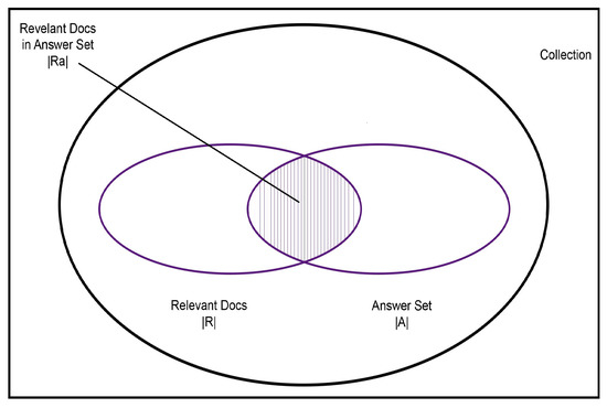
Figure 4.
Existing sets in a collection (Ra, R, A) (taken from [18]).
In Formula (7) the calculation of the memory is represented, where (response set of relevant images) and R (all relevant images), adapted from [18] is used, therefore it is defined that the memory is the fraction of the relevant documents from which they are recovered.
To obtain precision, the response set () and the response set (A) [18] are therefore used as the fraction of the documents retrieved with the relevant ones.
4.6. Neural Networks
An artificial neural network is a system that processes information the way a biological neural network works. Artificial neural networks have been developed as generalizations of mathematical models of human biological cognition because information processing occurs in many elements called neurons. The brain produces the signals that are passed between neurons through the connection links. Each connection link has a weight associated, which multiplies the transmitted signal, and each neuron applies an activation function to its input to determine its output signal.
The neural network consists of a large number of processing elements called neurons or nodes, each neuron is attached to other neurons through communication links, each with an associated weight, these weights represent the information used by the network to solve a problem, therefore, neural networks can be applied to various problems such as storage or retrieval of data or patterns, classification of patterns, grouping similar patterns, or finding solutions to optimization problems.
There are several variants such as self-organization maps (SOM) or back propagation, among others. Kohonen’s model (SOM) is based on the analogy of a topographic map, where we have n units of groups within an arrangement in one or two dimensions [19]. This model uses the vector of weights as input. The neural network model produces an associated particular group. During the training phase, the vector that most closely matches the input pattern is chosen as the winner neuron. In Figure 5, it is shown how the neighbors are grouped and a winning value is obtained forming a neighborhood.
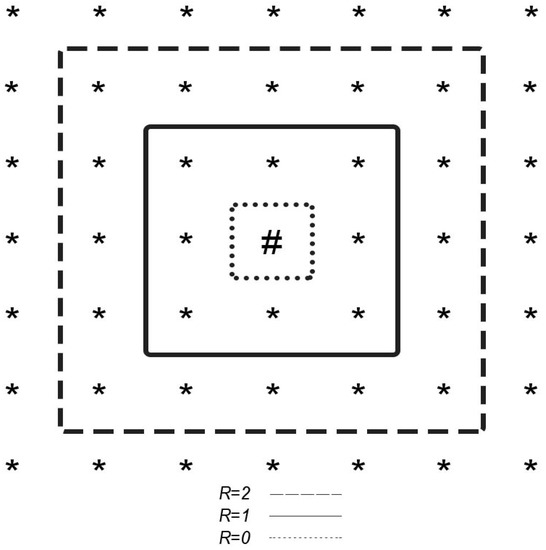
Figure 5.
Network of a rectangularly-generated neighborhood, where # is the winning value, ∗ are the neighboring values, points closest neighbors, line moderately close neighbors, and script farthest neighbors (taken from [19]).
To find the winning neuron, weights, entries, number of groups, the learning parameter, the initial radius and the number of categories (j) must be initialized. Each j is calculated with Formula (9), where w is the weight and x is the input at sample i in the input vector.
Once the minimum distance is found, the weights in Formula (10) are updated, but only for the winning unit, with being the learning parameter.
Finally, the learning parameter is updated and it is finished until the stop condition is met or until all the samples are provided to the neural network.
The back propagation model, also called generalizes delta rule, differs in that it is not a single layer but multilayer, like most networks. The objective of this is to train the network to achieve a balance between the ability to respond and the input patterns managing [19]. The back propagation training is of three stages, the first is the input training pattern feed, the second is the calculation and back propagation of the associated error, and the third is the adjustment of the weights.
The back propagation architecture is multilayer, as shown in Figure 6. This architecture can have one or more hidden layers (z units). The output and hidden units can have a bias that are denoted with b for the outputs and z for the hidden units.
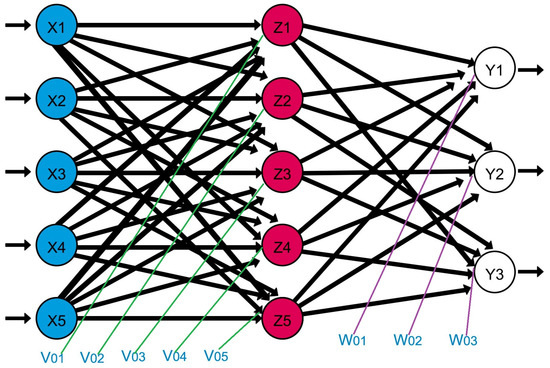
Figure 6.
Architecture of a back propagation neural network made up of five input neurons in the input layer in (blue), a hidden layer with five neurons in (red), an output layer with three neurons in white. The weight values with influence in the hidden layer are . The weight values with influence in the output layer are . Therefore, this neural network was designed for three classification groups, as can be observed in the output layer.
The process starts with the units that receive a signal that is transmitted to each unit of the hidden layer , each unit calculates its activation and sends it to the output units .
Then, their activation is computed from the network response for the input patterns. During training, each output unit compares its activation calculation with the target value to determine the associated error for each pattern.
The output and hidden units can have weights that are denoted with w for the output units and v for the hidden units, acting as weights among them.
Where it also calculates its activation from the network response for the input patterns. During training, each output unit compares its activation calculation with the target value to determine the associated error for each pattern.
Therefore, the hidden layer activation for units is denoted by the formula:
Its output signal is: . The output values of are denoted by Formula (12).
4.7. Decision Trees
Decision trees, as the name says, are used to make decisions on various topics where a value or several are sought. The values to classify are taken of electrophoresis samples. These trees can contain from 1 to n conditions or branches, a root node, a left sub-tree, and a right sub-tree. The objective of a binary tree is to search for a stored key, a sample of a decision tree can be observed in Figure 7.
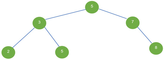
Figure 7.
Design of a binary decision tree where the node with value 5 is the root node, the node with value 3 starts the left sub-tree, the node with value 7 starts the right sub-tree, nodes with values 2, 5, and 8 are leaf nodes (taken from [20]).
To perform a search for a tree node, it is required that the pointer be at the root of the tree and trace a path. Each x will be compared to the key K until the value be found. Then, the pointer will return at the key node if it exists. If x is smaller than the key K, the search will be done in the left sub-tree, otherwise the search will be done in the right sub-tree. The nodes found during the recursion form a path down the root [20] this path will be taken as the runtime O (h) where h is the height of the tree. In the following listing, Listing 1, we have the pseudo code of a tree that performs a search.

Listing 1.
Tree basic algorithm [20].
Listing 1.
Tree basic algorithm [20].
| Tree-Search(x,k) |
| 1 if x=null or k= key[x] |
| 2 then return x |
| 3 if k < key[x] |
| 4 then return Tree-Search (left[x],k) |
| 5 else return Tree-Search (right[x],k) |
Decision trees, in addition to having major or minor decisions, can have numerical or boolean values. It is natural and intuitive to classify a pattern through a sequence of questions, in which the next query depends on the answer to the current question [21]. The type of decision can be answered with “yes/no” or “true/false” or “value (property)” or “set of values” based on comparisons.
5. Implementation of Smart Classification Paradigms with Wavelet Transformation
To perform the molecular weight measurement, four smart methods are applied. A content-based system, a back propagation neural network, a self-organizing-map-type neural network and a decision tree.
In the four intelligent paradigms, we start from a data set obtained from the electrophoresis samples. The data sets consist of the calculation of the wavelet transform that is obtained from the protein images.
Different types of wavelet transforms are calculated to know which one gives us a closer association with the values shown in Table 2. It is tested with the different parametric statistics thrown by the wavelets and compared against what is desired in the table, according to the values of the ranges and with prior knowledge of the molecular weights of the samples considered.

Table 2.
Table of ranges for the measurement of molecular weights (taken from [14]).
These experiments are taken from the research carried out by (Flores et al., 2019) [14] and for the reader’s convenience they are shown in Figure 8, Figure 9 and Figure 10. Wavelet calculations are performed with the Matlab R2014 Toolbox, as well as interface development and are explained below. As can be seen in Figure 8, the authors obtain the wavelet transformed from an electrophoresis sample and the level, channels, and protein points can be seen.
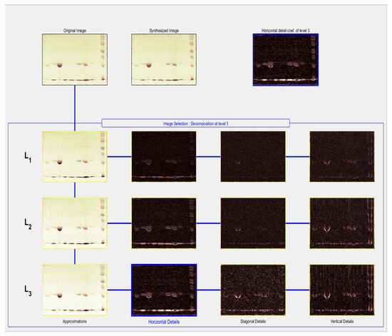
Figure 8.
Daubechies Wavelet Transform in the tree structure for level 3 of decomposition for electrophoresis samples (taken from [14]).
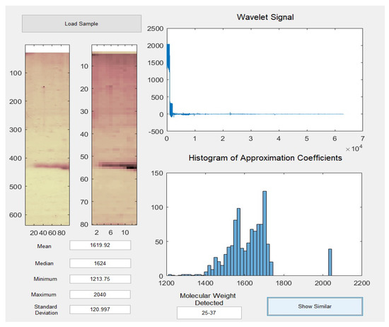
Figure 9.
Example of performance of the molecular weight detection system based on the wavelet transform taken from previous work done in [14].
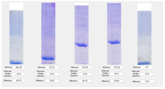
Figure 10.
Example of information retrieval for molecular weight measurement (taken from [14]).
Thirty samples are considered for the initial collection. The molecular weights are divides in four groups. In the first group of four samples, you have 15 kD. The second group of two samples has 20 kD of molecular weight. The third group of samples has 20 samples with 25 kD. Finally, the fourth group has four samples of 37 kD of molecular weights. In future work, 170 samples will be included.
The first paradigm with which the molecular weight measurement system is evaluated is the content-based approach. The second paradigm used is the neural network back propagation approach, followed by the self-organization maps approach. Finally, implementation through decision trees is shown in this section.
5.1. Content-Based Molecular Weight Measurement
Using the toolbox wavemenu in Matlab, in 2D mode, it is possible to observe the detection or better definition changes of the electrophoresis samples. The levels, the wavelet type, and the approximation or detail coefficients can be observed for your selection. In the same context, the calculated wavelet transform yields certain parametric statistics, which are considered to be analogous to the ranges of molecular weights in kilodaltons (kD).
The Daubechies transform at level 3 decomposition is then chosen, as well as its approximation coefficients.
The acquisition of each protein plate within the electrophoresis is created during four days of exposure. This indicates that obtaining each sample takes more than a month in laboratory work.
The statistics that are considered for the Daubechies approximation coefficients for each sample are: minimum, maximum, average, median, and standard deviation. An example of this can be seen in the interface shown in Figure 9, whose system was developed in a previous work [14] and is taken up as a starting point in this investigation.
The operation of the content-based system is as follows:
- (a)
- The image of the electrophoresis sample you want to analyze is loaded.
- (b)
- The image synthesized by wavelet is calculated.
- (c)
- The wavelet signal of the corresponding image is graphed.
- (d)
- The approximation coefficients histogram are displayed.
- (e)
- The minimum of the statistics for metrics are associated with a range of molecular weights.
- (f)
- The resulting molecular weight is thrown and goes to stage two of the system.
On the other hand, the second part of the content-based recovery system as the basis of this research, shown in Figure 10, taken from [14] is described below:
- (g)
- Once the molecular weight is measured, a distance measurement is calculated between the request image and the images contained in the sample bank.
- (h)
- The Euclidean metric is applied to calculate the differences.
- (i)
- Those five samples with the difference closest to zero are recovered.
- (j)
- The five most similar samples are displayed.
- (k)
- The minimum, molecular weight measured, and the difference are displayed.
- (l)
- The display order depends on the similarity against the request image in descending order.
There are different metrics to achieve a difference calculation by means of a correlation matrix. In the case of the system carried out in [14], the Euclidean metric is widely used for this type of task [18] and is expressed by the Equation (13):
With the CBIR-TW system, only the minimum parameter is used, and a successful image recovery is retrieved.
5.2. Back Propagation for Molecular Weight Measurement
The back propagation multilayer neural network which has five neuron for input layer, a hidden layer, equal to five nodes, and only four output nodes, which were also taken as the four groups of molecular weights. Hence, the architecture has the 5-5-4 configuration. The back propagation neural network is a supervised method. Figure 11 presents the results that it gave us when inserting the matrix of the 30 samples.
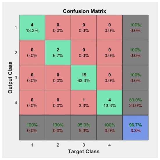
Figure 11.
Resulting confusion matrix with 30 samples to classify into four groups.
It is observed in the confusion matrix (see Figure 11) that 96.7% of correctly classified cases were obtained.
5.3. Self-Organization Maps for Molecular Weight Measurement
There are several variants of neural networks, in this research we chose the self-organization maps (SOM) as well. With the help of the toolbox provided by Matlab, we made the classifications of the four groups of molecular weights with which we worked in the previous paradigms. The matrix of the five parametric statistics of each electrophoresis sample (30 samples) were the input data for training phase. The matrix was obtained in the training, test, and validation phases (see Figure 1). The Daubechies approximation coefficients at decomposition in level 3 generates the approximation coefficients of each samples. The value of the mean, median, minimum, maximum, and standard deviation were the five inputs for the SOM network training. The behaviour of the input values to the neural network can be seen in Figure 12.

Figure 12.
Graphics of input plans of the Self Organization Maps neural network. From left to right, the four output nodes changes its color in function of learning process and its output value. The darkest values imply higher learning values, and brighter values, imply lower learning values.
SOM architecture uses a unsupervised approach in the training phase, because this neural network model decides how to classify at fly in each iteration.
The behavior of the weights of the SOM neural network is shown below, which marks point by point the displacement of the values of the weights that promote the final classification of the training (see Figure 13).
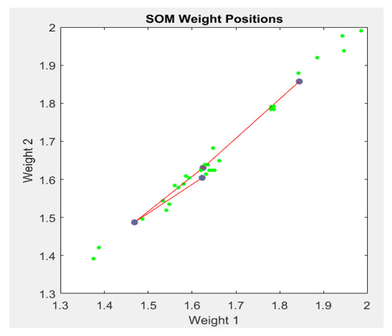
Figure 13.
Graphics of weight position of the matrix inserted as input.
5.4. Decision Tree for Molecular Weight Measurement
In the decision tree, the five parametric statistics were used, applying the J48 method in Weka (a workbench for machine learning created by Machine Learning Group at the University of Waikato [22]. The matrix generated by the approximation coefficients previously obtained were the input data for the tree decision.
Figure 14 shows the confusion matrix of the classified samples.
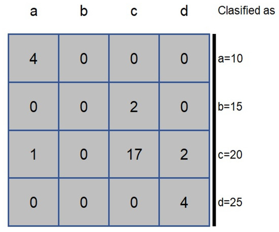
Figure 14.
Confusion matrix showing the classification of the 30 electrophoresis samples.
The matrix of confusion indicates how the 30 electrophoresis samples are classified into four groups, the same as in the previous method (10 kD, 15 kD, 20 kD, and 25 kD) where 25 samples were correctly classified and five were incorrect. This process is observed in Figure 15, which is the structure of the generated tree approach.
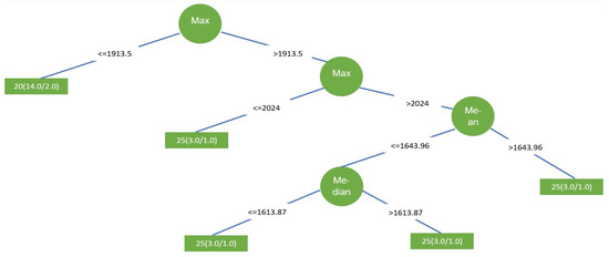
Figure 15.
Representation of decision tree for classification of molecular weights in four groups, taking into account 30 instances (samples) and the five characteristic data of each one.
6. Analysis of Results
In this research we have applied various classification paradigms such as a CBIR system, two methods of neural networks, and decision trees. The input data for all paradigms are wavelet transform in the Daubechies variant with the approximation coefficients of each electrophoresis sample. In the four methods that we applied, the same data set is used from 30 scanned electrophoresis samples.
The configuration of each of the paradigms is summarized below:
- The back propagation neural network was designed with a 5-5-4 architecture, because there are five characteristics considered in the input. There are five nodes in the hidden layer, which the programming used assigns by default. There are also four output nodes, which are precisely the molecular weight groups to be measured.
- In the case of the SOM neural network, it was designed with a 5-4 architecture, that is, there are no hidden layers, there are five input nodes (mean, median, minimum, maximum, and standard deviation). There is no hidden layer and there are four exit nodes, which are the four molecular weight groups that you want to measure.
- In the case of the decision tree, as can be seen in Figure 15, there are four nodes, which is the number of decisions that must be made to classify the measurements of the four groups of molecular weights. The tree is also fed with the five statistical variables that were already mentioned.
6.1. Analysis of Content-Based Paradigm Results
Regarding the results of the content-based approach, Table 3 shows the 30 samples, specifying their minimum value, their correct molecular weight, and the number of similar and non-similar samples obtained in the recovery of the CBIR paradigm previously reported in [14].

Table 3.
Samples with which the workouts were performed, their real molecular weight, their minimum value of the sample, how many similar and not similar of the five samples recovered, and the recall and precision are presented (taken from [14]).
To evaluate the performance of the CBIR paradigm, the recall and precision metrics are computed [17]. In the Figure 16 can be observed the recall and precision of retrieval of each query with 0.70 recall and 0.22 in precision.
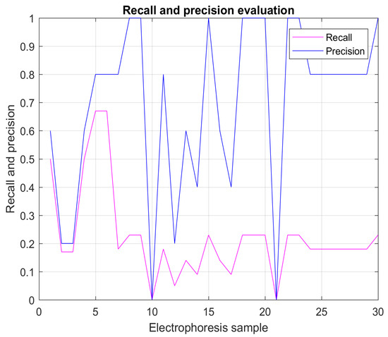
Figure 16.
Evaluation of recall precision metrics for the visual molecular weight detection (taken from [14]).
The value of Answer Set always will be of 5, because the system and the interface was programmed for to browse five retrieved images. Figure 16 graphically shows the results of the recall and precision evaluations obtained from the 30 electrophoresis samples.
In Table 3, (previously showed) we see all the results that were obtained, starting from the best precision measurement to the lowest.
6.2. Analysis of Back Propagation Neural Network Results
In the case of Backpropagation, the graphs of weights, input plans or sample hits are not provided by the Matlab Toolbox, and are replaced by the confusion matrix, the test graphs and the gradient graphs. That is the difference between supervised and unsupervised neural networks. In other words, not all neural network architectures are the same, their learning process is different, and the data they throw is different, even the way the Matlab Toolbox implements them, it also differs. This is the reason why we do not provide the same graphs for both neural network models.
On the other hand, in back propagation, a better classification/precision percentage of 96.7% was obtained, this being the best percentage of all the paradigms applied in this investigation. This neural network uses a supervised approach and shows the learning behaviour for the training set (blue line), validation set (green line), testing set (red line) and a fourth training set that put together all sets (black line) in Figure 17.
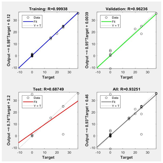
Figure 17.
Learning graphs of the four validation tests of back propagation generated by the Matlab Toolbox.
We observed that in the performance of the training phase, most of the cases remained close to or within the optimal results line. In the training phase, there was a small change in the direction of the fit and four cases moved away from the optimal line with an error of 0.99938 (see Figure 17 up and left). For the validation phase (Figure 17 up and right) the greatest change in the direction of the fit line was noted, and four molecular weights were not correctly classified and an error of 0.9636 was obtained. In the test phase (Figure 17 down and left), six items were misclassified, so the error is 0.68749. Finally, it is shown in Figure 17 down and right that the error for three phases is of 0.93251.
In Figure 18, we observe the gradient of the neural network, showing that the learning in epoch 17 stabilizes and begins to drop, so the training stops to prevent learning from falling to a local minimum.

Figure 18.
Back propagation learning gradient.
6.3. Analysis of Self-Organization Neural Network Results
The Sample Hits section (see Figure 19) provides the groups that where classified, that is, if we classify into four groups, the 30 samples that make up the matrix must fall in one of those four groups.
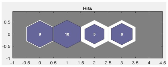
Figure 19.
Thirty hits classified in four groups through five input nodes.
We know that of the 30 samples, 20 are of a molecular weight of 25 kD, two of a molecular weight of 20 kD, and the remaining eight are of the two groups of 15 kD and 37 kD. Therefore, in the classification of the output nodes of the SOM neural network (see Figure 19), the groups of 15, 20, and 37 kD were classified correctly. In the group of 25 kD, only 50% of the samples were classified correctly and the remaining 10 were scattered in the other three groups. That misclassification made the SOM only 66% accurate.
With the SOM neural network, a classification/precision of 66% was obtained, which presented a greater number of badly classified samples.
6.4. Analysis of Results for the Tree Decision
The results obtained by this paradigm are those shown in Table 4.

Table 4.
Weka J48 training set results.
When classifying the 30 samples, an 83.33% correct classification was obtained by decision tree approach using J48 algorithm.
6.5. Analysis of Results for the Four Paradigms
With the application of these four paradigms (Table 5), three of them exceeded 80% of accuracy classification, with the back propagation neural network and the CBIR system being those that exceeded 90% of classification. The back propagation paradigm had the best percentage.

Table 5.
Results of the four paradigms applied in the classification of molecular weights.
The back propagation neural network was designed with a 5-5-4 architecture, because there are five characteristics considered in the input. There are five nodes in the hidden layer, which the programming used assigns by default. There are also four output nodes, which are precisely the molecular weight groups to be measured. In the case of the SOM neural network, it was designed with a 5-4 architecture, that is, there are no hidden layers, there are five input nodes (mean, median, minimum, maximum and standard deviation). There are four exit nodes, which are the four molecular weight groups that you want to measure. In the case of the decision tree, as can be seen in Figure 15, there are four nodes, which is the number of decisions that must be made to classify the measurements of the four groups of molecular weights. The tree is also fed with the five statistical variables that were already mentioned and the generation of nodes takes place according to the ranges included in the statistical data.
From a technical point of view, it is possible to reproduce the previously detailed experiments. This is possible, through any other collection of scanned electrophoresis images. The images can be produced in an industrial chemistry laboratory. Protein samples can be extracted from food, plants, or tissue samples from various sources. Once obtained, they can be converted to gray levels and subsequently analyzed by a transformed wavelet Daubechies. The molecular weight can be calculated using the equivalence values shown in Table 2 proposed in this article. These equivalences cover the molecular weight readings or ranges comparable to the most commonly used commercial markers using the minimum of the coefficient wavelet transforms for all paradigms as main parametric statistic.
To obtain the electrophoresis samples, a long process is required, because this involves several steps for its realization. The process that requires more time is when the sample is placed in the solution. Then, the revealing solution helps to clean up the analysis and only leaves the areas that contain information on the proteins. This process involves about 96 hours (approximately four days), so the obtainment of each one of the 30 samples for the experiments in Table 3 is not a trivial task.
The experimentation stage faced a challenge at the moment of producing the samples, which consisted in that the electric field supply, in many occasions, caused the loss of the same, due to the excess voltage. Because of this, the samples were discarded. Subsequently, the processing part involved the cutting of each of the samples, and standardized each image for analysis, that is, each image had to be cut with a measurement in pixels of 100 pixels wide by 700 pixels long, approximately.
To perform the selection of the wavelet transform, Haar, biorthogonal, and Daubachies were tested, achieving similar results. However, only the Daubechies results are shown, because the visual coefficients of greater importance in the protein signal content highlight the molecular weight score. Then, the decomposition levels are analyzed, where the wavelet transform Daubechies showed with a higher illumination, the said protein score. On the other hand, the parametric statistics and the histograms obtained established an analogy between the detection of molecular weights and the electrophoresis samples.
With the variant Daubechies to a level of decomposition 3, the approximation coefficients of each sample were obtained. From Wavelet Daubechies Transform were obtained parametric statistics such as the mean, the median, the minimum value, maximum, and standard deviation. Of these five statistics, which are considered as characteristics of the image, only in the case of the minimum value, a correspondence of molecular weight is found. The other characteristics did not show much correspondence for the correct detection of molecular weights, because there were no predefined ranges, the readings were spliced or there was definitely no adequate correspondence.
Within the 30 experiments that are observed in Table 3, in 93% of the cases, at least one image corresponds effectively to the molecular weight that the users want to find or compute, that is, the system recovers statistics and at least one sample of molecular weight similar to the query sample. The recall value is 0.22 and precision value is 0.70, and can be observed in Figure 16. It is important to mention that in a content-based system, the maximum value in recall is 0.5, and the maximum value in precision is 1.0.
This indicates that it can also be observed that in each of the requests for molecular weights, recall and precision are measured. In each of the 30 cases taken at random, we can see that while the precision is closer to 1.0 indicates that the search was more accurate. If the recall is closer to 0.5, this implicates that the number of similar images was higher or more efficient visually and statistically speaking.
The back propagation neural network uses supervised learning. The accuracy of classification was of 96.7%. The 29 electrophoresis samples were classified in the corresponding group, only one was out of the classification (see Figure 11). The groups that had all the cases classified in the correct group were those of molecular weight 15, 20, and 37 kD.
In the self-organization neural network, the same data set was inserted as in the previous methods, for the input nodes of the network. Ten missing samples were wrongly classified among the other groups: two in the 15 kD group, three in the 20 kD group, and five in the 37 kD group. Then, most of the samples were classified in the groups close to the 25 kD.
In the decision tree, J48, the WEKA software, and the matrix of the 30 samples are used. The five parametric statistics were used (minimum, maximum, mean, median, and standard deviation). By using the five statistics, the correct classification was exceeded at 83.3%. Only three samples of 25 kD molecular weight were not classified in the correct group.
7. Conclusions
Of the four paradigms that were applied to classify and detect molecular weight, three of them exceeded 80%, these were CBIR, back propagation, SOM, and J48, where in CBIR-WT only the minimum value was used, the other three used five statistics. Neural networks turned out to have the best paradigm for back propagation and the worst paradigm for SOM, back propagation was the best with 96.7% of correct classification, since this variant is supervised learning. On the other hand, SOM obtains a percentage of 66%.
Regarding the hypothesis that arose at the beginning of this investigation, we can point out that a measurement of molecular weights is achieved and a recovery of images similar to the molecular weight that is desired to be measured with 96% accuracy under an intelligent paradigm such as back propagation.
The greatest findings achieved in this work lie in the fact that the field of measurement of molecular weights has not yet been widely studied at a scientific level, much less under intelligent paradigms. However, it is important to note that there are commercial versions which have high costs or whose maintenance requires additional costs. Another important finding is that parametric statistics of low wavelet transform electrophoresis is viable for molecular measurement. It was also found that intelligent paradigms are effective for this type of measurement, but that back propagation was better than others such as trees, or even better than other types of neural networks or content-based systems.
The main contributions to the area are focused on a visual information retrieval system that can accompany a measurement of molecular weights by means of wavelet transform Daubechies, Haar, and biorthogonal. Another of the main contributions is to provide a content-based tool to find molecular samples similar to those to be measured. This may lead to future work such as comparisons of food proteins, drugs, human tissue for testing of new drugs, or the search for more nutritious foods for human consumption, to name a few. Evolutionary optimization paradigms may also be tested in the future, which will improve measurement results in molecular weights.
Finally, it should be mentioned that among the initial limitations or conditions of the research, the limited number of samples available must be taken into account, since in this work there were a total of 29 to 30 samples and 10 of them were rejected as illegible. Furthermore, the the number of days involved in obtaining a single sample must be taken into account, since normally obtaining a single sample takes between four and five days. The measurement of the revealing plates for electrophoresis regarding the pore size allows the displacement of the molecules to be measured, and that in this work, the pore measurement was 12%.
Author Contributions
The individual contributions are detailed as follows: Software, investigation, writing, formal analysis and preparation of original draft, J.A.F.-L. Conceptualization, methodology, review, editing and supervision: L.F.-P. Validation, resources and data curation: L.P.J.-Q. Resources: C.R.S.-P. All authors have read and agreed to the published version of the manuscript.
Funding
We thank Carolina Rocío Sánchez Pérez, coordinator of the Computer Engineering education program and Laura Patricia Jaramillo Quintero, Coordinator of the Industrial Chemistry educational program, for their support in the dissemination and publication of this work research.
Acknowledgments
We thank Laura Patricia Jaramillo Quintero, for her help in carrying out the electrophoresis experiments and part of the equipment and materials used in this research.
Conflicts of Interest
The authors declare no conflict of interest.
Abbreviations
The following abbreviations are used in this manuscript:
| CBIR | Content-Based Image Retrieval |
| WT | Wavelet Transform |
| DAUB1Ln | Daubechies WT, type 1, Level of decomposition n |
| HAAR1Ln | Haar WT, type 1, Level of decomposition n |
| BIOR1Ln | BIOR WT, type 1, Level of decomposition n |
| CBIR | CBIR System |
| SOM | Self-Organization Maps |
| ANN | Artificial Neuronal Network |
| GA | Genetic Algorithm |
| ANFIS | Adaptative Neuro-Fuzzy Inference System |
| CHAID | Chi-Square Automatic Interaction Detection |
| SDS | Sodium dodecylsulfate |
| PAGE | Poliyacrylamide Gel |
References
- Horton, R. Principios de Bioquímica, 4th ed.; PEARSON Educación: Mexico City, México, 2008. [Google Scholar]
- González, R.C.; Woods, R.E. Digital Image Processing, 3rd ed.; PHI Learning: New Delhi, India, 2008. [Google Scholar]
- Zhan, X.; Zhou, T. Application of Two-dimensional gel electrophoresis in combination with mass spectrometry in the study of hormone proteoforms. In Mass Spectrometry: Future Perceptions and Applications; Kamble, G.S., Ed.; InTech-Open Science Publisher: London, UK, 2018; ISBN 978-953-51-7845-3. [Google Scholar]
- Kahlenberg, F.; Sack, U.; Bolt, A. Impact of image analysis software on quantitations of 1D gel electrophoresis. J. Lab. Med. 2012, 36, 153–157. [Google Scholar]
- Reza-Sohrabi, M.; Muzabeygi, V.; Davallo, M. Use of continuous wavelet transform approach for simultaneous quantitative determination of multicomponent mixture by UV-Vis spectrophotometry. Spectrochim. Acta Part A Mol. Biomol. Spectrosc. 2018, 201, 306–314. [Google Scholar] [CrossRef] [PubMed]
- Zhou, W.; Zheng, B.; Liu, Y.; Wang, C.; Sun, W.; Li, W.; Chen, S. Advances in capilarlly electrophoresis spectrometry for cell analysis. Trends Anal. Chem. 2019, 117, 316–330. [Google Scholar] [CrossRef]
- Salazar-Centeno, C.A.; Niño-Niño, C.A.; Diaz-Suarez, R.A. Detección de bandas de color en una imagen de electroforesis en gel de una dimensión usando un algoritmo de localización basado en máximos y mínimos. Iteckne 2017, 14, 12–30. [Google Scholar] [CrossRef][Green Version]
- Liu, P.; Miau, Z.; Guo, H.; Wang, Y.; Ai, N. Adding spatial distribution clue to aggregated vector in image retrieval. EURASIP J. Image Video Process. 2018, 9, 1–14. [Google Scholar] [CrossRef]
- Rahmani, R.; Niazi, P.; Naseri, M.; Neishabouri, M.; Farzanefar, S.; Eftekhari, M.; Derakhshan, F.; Mollazadeh, R.; Meysami, A.; Abbasi, M. Precisión diagnóstica mejorada para la imagen de per-fusión miocárdica usando redes neuronales artificiales en diferentes variables de entrada incluyendo datos clínicos y de cuantificación. Rev. Esp. Med. Nucl. Imagen Mol. 2019, 38, 275–279. [Google Scholar] [PubMed]
- Bollado, J.; Marco-Ahulló, A.; Villarrasa-Sapiña, I.; Gonzalez, L.M.; García-Massó, X. Dolor de espalda en estudiantes de entre 12 y 17 años: Aproximación multifactorial basada en árboles de decisión. Fisioterapia 2018. [Google Scholar] [CrossRef]
- Gudelis, M.; Lacasta Garcia, J.D.; Trujillano Cabello, J.J. Dolor agudo en fosa ilíaca derecha. Un nuevo algoritmo de diagnóstico basado en árboles de clasificacioón y red neuronal artificial. Cir. Esp. 2019, 97, 329–335. [Google Scholar] [CrossRef] [PubMed]
- Sprockel Diaz, J.J.; Diaztagle Fernandez, J.J.; Gonzalez Guerrero, E. Diagnóstico automático del sindrome coronario agudo utilizando un sistema multiagente basado en redes neuronales. Rev. Colomb. Cardiol. 2017, 24, 255–260. [Google Scholar] [CrossRef]
- Nwobi-Okoye, C.C.; Quent Ochieze, B.; Okiy, S. Multi-objetive optimization and modeling of age hardening process using ANN, ANFIS and genetic algorithm: Results from aluminum alloy A356cow horn particule composite. J. Mater. Res. Technol. 2019, 8, 3054–3075. [Google Scholar] [CrossRef]
- Flores-Lopez, J.A.; Flores-Pulido, L.; Jaramillo-Quintero, L.P. Molecular Marker for Proteín Electrophoresis by Wavelet Transform. Res. Comput. Sci. 2019, 148, 21–34. [Google Scholar] [CrossRef]
- Walker, J.S. A Primer on Wavelet and Their Scientific Applications, 2nd ed.; CRC Press: Boca Raton, FL, USA, 2008. [Google Scholar]
- Misti, M.; Misti, Y.; Oppenheim, G.; Poggi, J.M. Wavelet Toolbox for Use with Matlab, 2nd ed.; The Mathworks Inc.: Natick, MA, USA, 2016. [Google Scholar]
- Chen, Y.; Li, J.; Wang, J.Z. Machine Learning and Statistical Modelling Approaches to Image Retrieval; Kluwer Academic: Norwell, MA, USA, 2004; p. 182. [Google Scholar]
- Baeza-Yates, R.; Ribeiro-Neto, B. Modern Information Retrieval; ACM Press, Addison-Wesley: Edinburgh, UK, 1999; p. 340. [Google Scholar]
- Fausset Laurene, V. Fundamentals of Neural Networks: Architectures, Algorithms, and Applications; Prentice Hall: Upper Saddle River, NJ, USA, 1994. [Google Scholar]
- Cormen Thomas, H.; Leiserson Charles, E.; Rivest Ronald, L. Introduction to Algoritms; The Massachusetts Institute of Technology Press: Cambridge, MA, USA, 1990. [Google Scholar]
- Duda, R.O.; Hart, P.E.; Stork, D.G. Pattern Classification, 2nd ed.; John Wiley and Sons: New York, NY, USA, 2001. [Google Scholar]
- Bouckaert, R.R.; Frank, E.; Hall, M.; Kirkby, R.; Reutemann, P.; Seewald, A.; Scuse, D. WEKA Manual for Version 3-8-3. Available online: https://sourceforge.net/projects/weka/files/weka-3-8/3.8.3/ (accessed on 14 September 2018).
© 2020 by the authors. Licensee MDPI, Basel, Switzerland. This article is an open access article distributed under the terms and conditions of the Creative Commons Attribution (CC BY) license (http://creativecommons.org/licenses/by/4.0/).