Neural Network Approach to MPPT Control and Irradiance Estimation

Abstract

Photovoltaic (PV) modules require maximum power point tracking (MPPT) algorithms to ensure that the amount of power extracted is maximized. In this paper, we propose a low-complexity MPPT algorithm that is based on the neural network (NN) model of the photovoltaic module. Namely, the expression for the output current of the NN model is used to derive the analytical, iterative rules for determining the maximal power point (MPP) voltage and irradiance estimation. In this way, the computational complexity is reduced compared to the other NN-based MPPT methods, in which the optimal voltage is predicted directly from the measurements. The proposed algorithm cannot instantaneously determine the optimal voltage, but it contains a tunable parameter for controlling the trade-off between the tracking speed and computational complexity. Numerical results indicate that the relative error between the actual maximum power and the one obtained by the proposed algorithm is less than 0.1%, which is up to ten times smaller than in the available algorithms.

1. Introduction

Solar energy plays a significant role in electricity production nowadays, due to its sustainability and abundance, simple installation of photovoltaic (PV) systems, reliable non-polluting power generation, etc. Accurate modeling of the PV cell/module is extremely important for optimal design and evaluation of PV systems. Various equivalent electrical circuits for photovoltaic cell/module modeling have been presented in the literature. Among them, a five-parameter single-diode model is commonly used, due to its low complexity and satisfactory accuracy [1]. Hence, many techniques have been proposed for the extraction of those five parameters: some perform the parameter extraction based on the manufacturer datasheet information [2,3,4], while the others obtain the parameters using a set of experimental current-voltage (I-V) points [5,6,7]. Moreover, the methodologies that utilize both the datasheet and experimental data to extract the unknown parameters are also available in the literature [8]. The equivalent PV circuit is described by a set of transcendental equations, which are solved by iterative numerical procedures [9]. The closed-form solution of I-V characteristics can be obtained by utilizing the Lambert W function [9,10].

Besides the electrical equivalent, the data-driven PV cell modeling approaches have also been suggested by several authors. Those techniques perform PV model identification directly from the measured data and usually have higher accuracy [11,12]. In [13], the PV cell is modeled by using the Multilayer Neural Networks, while in [14,15] authors use the generalized regression and radial basis function neural networks. Recently, a one-dimensional deep residual network framework has been applied to the PV modeling problem [16]. A data-driven method based on the simple linear regression and smoothing spline has been proposed in [17], while a hybrid approach, which combines the benefits of neural networks and fuzzy logic, is given in [18].

PV cells require maximum power point tracking (MPPT) algorithms to ensure that the amount of power extracted is maximized. The maximum power point (MPP) changes with irradiance and temperature variations, and, therefore, it is important to develop the MPPT algorithms that will be fast enough to track these changes. Since, in general, the MPPT algorithms can be classified in different ways, in this paper we will divide them into two categories: model-free and model-based methods. The only prerequisites for implementing model-free algorithms are current and voltage measurements, without compulsory information of the PV model. The implementation of these algorithms is cost-effective; however, they have disadvantages such as oscillations around the MPP, slow convergence speed, and poor performance under the rapid change of the irradiance. Among these methods, the most popular are the Perturb and Observe (P&O) [19,20,21,22] and Incremental Conductance algorithm [23,24]. Recently, many algorithms that use different optimization techniques have been proposed to solve the MPPT problem under non-uniform irradiance conditions [25,26,27].

The model-based MPPT algorithms utilize the photovoltaic model to determine the MPP position. These methods exhibit fast tracking speed and high efficiency in the steady-state, but usually have greater complexity. In [28], the MPPT algorithm that uses the polynomial approximation of the equivalent circuit equations has been proposed, while the algorithm that relies on the exact closed-form solution based on Lambert W-function can be found in [29]. Many model-based MPPT algorithms that use neural networks have also been proposed in the literature [30]. The neural network (NN)-based algorithms provide the MPP voltage at the output, while their inputs can be datasheet information [31,32,33], irradiance and temperature [34,35,36], voltage and current measurements [37,38]. Among them, the most promising are algorithms that do not use irradiation measurements, because irradiance sensors are costly and difficult to calibrate. It has been shown that the usage of the irradiance sensors can be effectively avoided by using the irradiance estimators [29,39,40,41]. However, implementation of the irradiance estimators additionally increases the computational cost.

Here we propose a simple MPPT algorithm that is based on the neural network (NN) model of the photovoltaic module. The expression for the output current of the NN model is used to develop am analytical, gradient MPPT algorithm, which can provide high prediction accuracy of the maximal power. Finally, to avoid the usage of the pyranometer, a simple irradiance estimator, which is also based on the identified NN model, has been proposed. The presented algorithm has smaller computational complexity compared to the other NN-based MPPT algorithms, in which the MPP position is predicted by one multilayer NN or by two single-layer NNs. The performance improvement of the proposed approach over the available methods is confirmed by numerical examples with simulated and experimental data.

The rest of the paper is organized as follows: The procedure of modeling the photovoltaic cell/module and MPPT problem are described in Section 2. The proposed MPTT algorithm and irradiance estimator are presented in Section 3. This is followed by numerical results and discussion in Section 4 and Section 5.

2. Theoretical Background

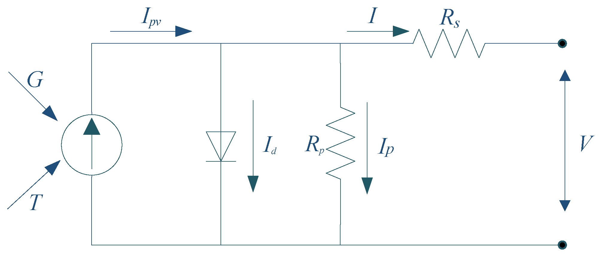
2.1. Equivalent Electrical Circuit of PV Module

The photovoltaic module is commonly modeled in literature with a single-diode circuit shown in Figure 1 [1]. The relation between the module terminal current and voltage is given by:

$$I=I_{pv}-I_s\left[exp\left(\frac{V+I{R}_s)}{V_t}\right)-1\right]-\frac{V+I{R}_s}{R_p}.$$

(1)

where I is the output current of the module, V is the output voltage, $I_{pv}$ is the photocurrent, $R_p$ is a shunt resistance, $R_s$ is a series resistance, $I_s$ is the diode saturation current, and $V_t$ is the thermal voltage. The thermal voltage is equal to $V_t=nkT{N}_s/q$, where q is the electron’s elementary charge [$=1.602\times {10}^{-19}\mathrm{C}]$, k is the Boltzman constant [$=1.381\times {10}^{-23}\mathrm{J}/\mathrm{K}$], T is the temperature of the cell [40], and $N_s$ is the number of series solar cells in a PV module.

The equivalent circuit has five unknown parameters that need to be determined. Generally, the  parameters of the PV module depend on the environmental conditions, especially on the irradiance (G) and module temperature (T). The parameters $I_{pv}$, $I_s$, $V_t$ and $R_p$ for different working conditions can be expressed as [40]:

$$I_{pv}=\left(I_{pv,ref}+\alpha (T-T_{ref})\right)\frac{G}{G_{ref}},$$

(2)

$$I_s=I_{s,ref}{\left(\frac{T}{T_{ref}}\right)}^{3}exp\left(\frac{q{E}_q}{nT}\left(\frac{1}{T_{ref}}-\frac{1}{T}\right)\right)$$

(3)

$$V_t=V_{t,ref}\left(\frac{T}{T_{ref}}\right)$$

(4)

$$R_p=R_{p,ref}\left(\frac{G_{ref}}{G}\right)$$

(5)

where index $ref$ denotes parameters values measured under standard test conditions (STC), defined at ambient temperature 25 ${}^{\circ }$C and irradiance 1000 $\mathrm{W}/{\mathrm{m}}^2$. The short-circuit current temperature coefficient is denoted by $\alpha$, whereas $E_g$ is the bandgap energy of the semiconductor.

Figure 2 shows the typical P-V characteristic of the PV module for different values of temperature and irradiance. It can be seen that the position of the MPP changes as a function of irradiance and temperature.

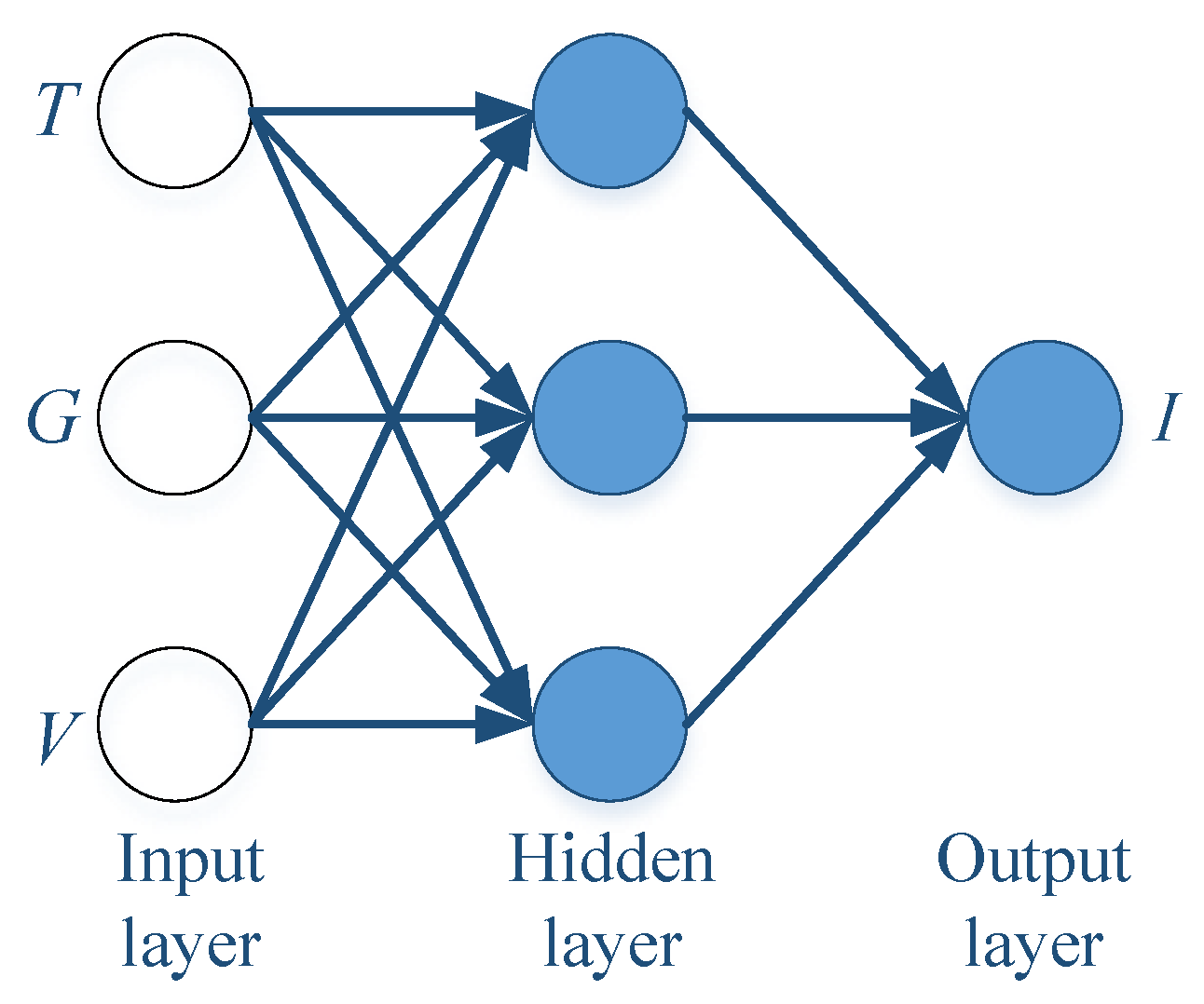
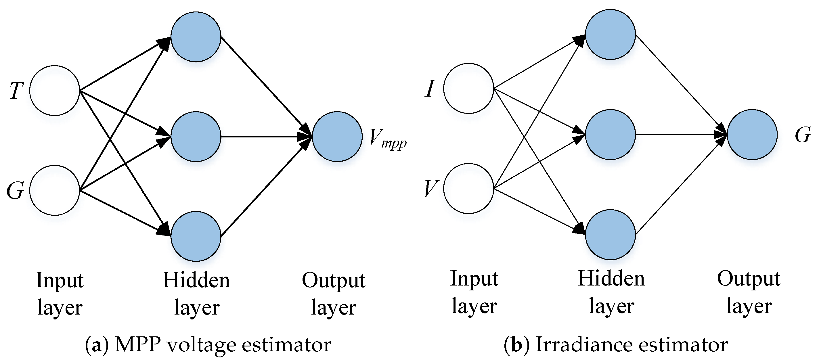
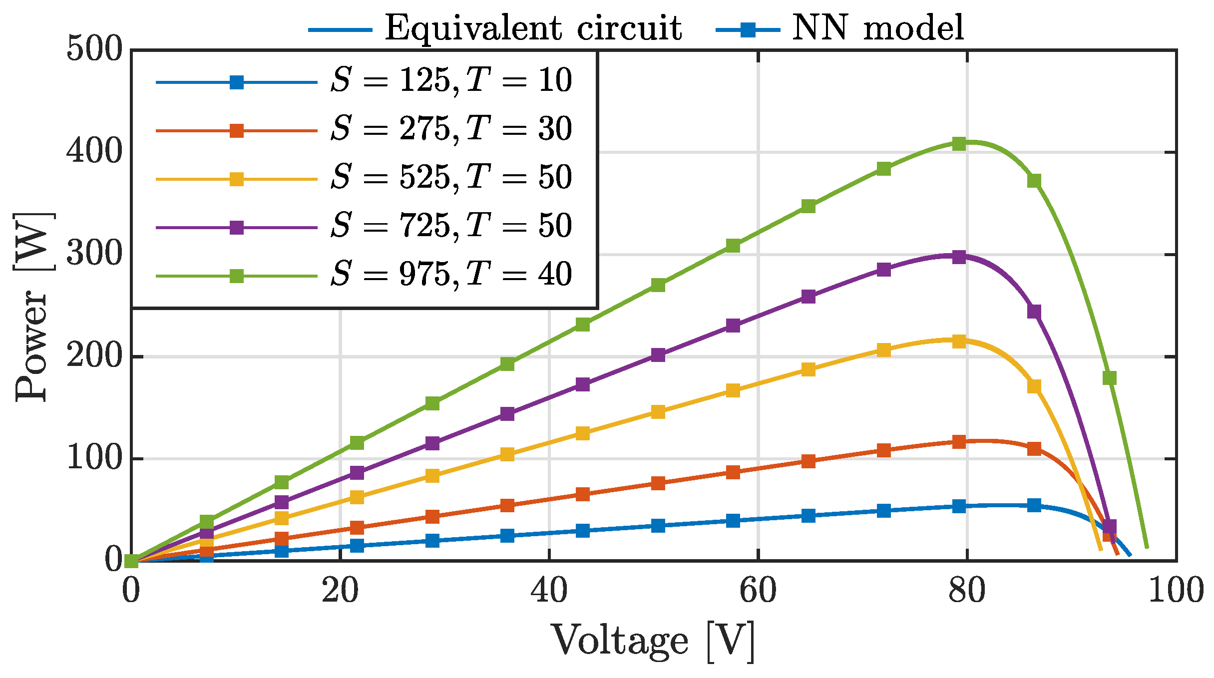
2.2. Neural Network Model of PV Module

In recent years, neural networks (NN) have been increasingly applied to various engineering problems, due to their capability to solve complex and nonlinear problems. In general, authors have proposed the usage of different NN architectures for photovoltaic modeling [11,12,13,14,15]. Here we detail the procedure of photovoltaic modeling with one-hidden-layer feedforward NN, because this network later will be used for the design of the MPPT algorithm and irradiance estimator.

The feedforward NN model with one hidden layer and three neurons is shown in Figure 3. The solar irradiance G, temperature T and voltage V represent inputs to the neural network, while the module current I is chosen as output. The output current of the NN model is given by:

$$\widehat{I}=net\left(\mathbf{u}\right)={\mathbf{W}}_{\mathbf{2}}tanh\left({\mathbf{W}}_{\mathbf{1}}\mathbf{u}+{\mathbf{b}}_{\mathbf{1}}\right)+{\mathit{b}}_{\mathit{2}},$$

(6)

where $\mathbf{u}={\left[\begin{array}{ccc}T& G& V\end{array}\right]}^T$, whereas ${\mathbf{W}}_{\mathbf{1}},{\mathbf{W}}_{\mathbf{2}},{\mathbf{b}}_{\mathbf{1}}$ and $b_2$ are the coefficients that need to be learned from the available input/output training sets.

In order to facilitate the learning process, each input can be normalized by using the formula:

$$u_{i,new}=\frac{u_i-u_{i,min}}{u_{i,max}-u_{i,min}},i\in \left\{S,T,V\right\},$$

(7)

where index $max$/$min$ denotes the maximal/minimal value of $S,T,V$ in the training set. A similar operation can be performed with the output training data.

The neural network coefficients are optimized by using the Levenberg–Marquardt algorithm or some other second-order algorithm. The cost function is defined as the mean square error (MSE) between the predicted and actual current:

$$J=\frac{1}{{\sum }_{i=1}^M{N}_i}\sum _{i=1}^M\sum _{k=1}^{N_i}{(\widehat{I}-I)}^2$$

(8)

where $N_i$ is the number of available points of I-V curve for specific irradiance $G_i$ and temperature $T_i$, while M denotes the number of different I-V curves.

Operating points making up the training set may be collected by experiments under controlled environmental conditions [17]. The environmental data need to be uniformly distributed in order to avoid overfitting/underfitting in the ranges that have more/less training data. Moreover, it is important to cover all G and T values that can occur in practical scenarios, because the NNs do no have good extrapolation properties. In case that only a small amount of experimental data or manufacturer datasheet information is available, the parameters of the equivalent circuit should be determined first. After that, the training data can be synthesized by using Equations (1)–(5). However, it has been shown that the PV models built directly from the measured data usually have greater accuracy than the equivalent circuit models [16].

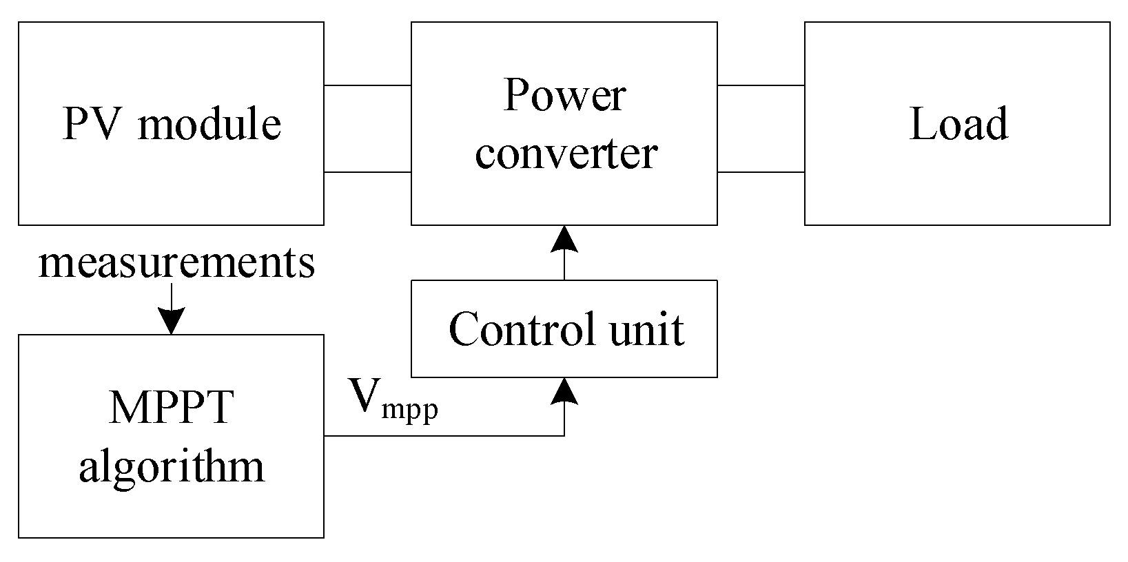
2.3. Overview of MPTT Algorithms

The MPPT tracker system is usually composed of the MPPT algorithm, power converter, and control unit (Figure 4). The MPPT algorithm aims to provide the MPP voltage ($V_{mpp}$), which is used as the reference value in the power converter control loop. Due to simplicity, it can be assumed that the power converter is perfectly controlled.

One of the simplest MPPT algorithms is the Perturb and Observe (P&O) [20]. The P&O is the model-free algorithm that iteratively changes the output voltage towards the MPP, wherein the direction of change is determined by using the voltage and current measurements. The main limitations of the model-free algorithms are slow tracking speed and steady-state oscillations about the MPP [20]. The MPPT algorithms that rely on the photovoltaic model can be used to deal with these issues [28,29]. The model-based algorithms are fast and accurate, but also more complex and require irradiance sensors for implementation. The irradiance sensors are costly and difficult to calibrate. However, it has been shown that the irradiance sensors can be effectively replaced by irradiance estimators [29].

On the other hand, as far as the model-based algorithms are concerned, not only are there MPPT algorithms based on the equivalent circuit models, but there are also many of them based on neural networks. Comprehensive review of the NN-based MPPT algorithms can be found in [30]. The NN-based algorithms provide the $V_{mpp}$ voltage at the output, while their inputs can be datasheet information [31,32,33], irradiance and temperature [34,35,36], voltage and current measurements [37,38]. Moreover, some authors focuses on the design of both the MPPT algorithm and control unit [42,43]. Hybrid approaches that combine the NN-based algorithm with model-free algorithms have also been proposed [44].

Among the proposed algorithms, the most precise are those that use irradiance and temperature as input information [34,35,36]. Figure 5a shows an example of the feedforward NN in which G and T measurement are used to predict $V_{mpp}$. It should be noted that other types of networks, such as a radial basis function NNs, can be used in the same way. The NN from Figure 5a provides the $V_{mpp}$ instantaneously, which enables fast tracking speed under fast changes of the environmental conditions. However, the drawback of this algorithm is that the irradiance information needs to be known. In [38], a cascade NN-based MPPT (CNNMPPT) the technique is proposed where two NNs are utilized to estimate $V_{mpp}$. The first NN estimates the irradiance from the voltage and current measurements (Figure 5b), whereas the other NN determines the MPP voltage from the temperature and estimated irradiance (Figure 5a). The proposed technique can provide accurate results, but at the cost of the increased computational complexity. The algorithm that predict the MPP voltage by using the multilayer feedforward NN is proposed in [33].

3. Proposed MPPT Algorithm and Irradiance Estimator

Here we propose a low-complexity MPPT algorithm and an irradiance estimator with the aim of improving the MPP voltage prediction accuracy. Unlike the available NN-based algorithms that directly determine the MPP voltage from the measurements, the proposed algorithm relies on the NN model of the PV module, described in Section 2.2. Namely, the expression for the output current of the NN model is used to derive the analytical, iterative rules for determining the MPP voltage and irradiance estimation. The proposed solution has smaller computational complexity compared to the available NN-based algorithms that use the same input information. While other solutions use one multilayer NN or two single-layer NNs, the proposed technique relies on the NN-model that can be trained accurately with 4 neurons in the hidden layer. The proposed algorithm cannot instantaneously determine the optimal voltage, but it has a tunable parameter that can be used to control the trade-off between the tracking speed and computational complexity.

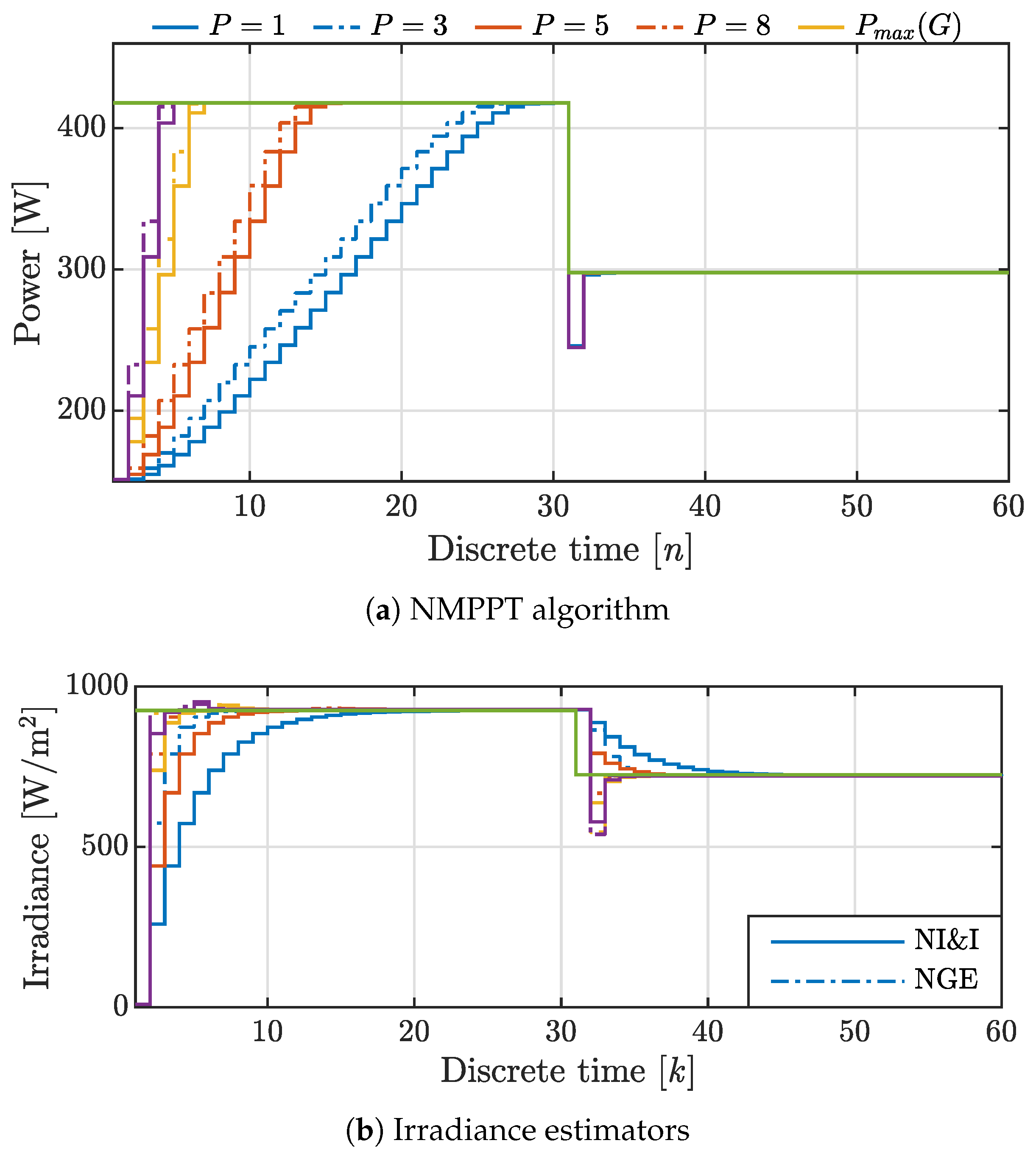
3.1. NMPPT Algorithm

The relation between the photovoltaic output power, current and voltage is given by:

$$P=V·I=V·I(V,S,T).$$

(9)

The aim of the MPPT algorithm is to find the point ($V_{mpp}$, $I_{mpo}$) at which the output power P is maximal:

$$P_{mpp}=P(V_{mpp},I_{mpp})\ge P(V,I),\forall V,I.$$

(10)

It is well known that, under the uniform irradiance condition, the P-V curve is strictly concave, which can be observed from Figure 2. Thus, the MPP can be found by the means of the gradient ascend rule:

$$V_{k+1}=V_k+\mu \frac{\partial P_k}{\partial V_k}=V_k+\mu \left(I_k+V_k\times \frac{\partial I_k}{\partial V_k}\right)$$

(11)

where k is the discrete time-instant, while $\mu$ is the positive step size that controls the convergence speed. The algorithm will converge faster for the larger step size, but it will also be more sensitive to the measurement noise. There is no exact analytical approach for determining the maximal value of $\mu$, but it can easily be tuned experimentally. As the rule of thumb, the function that changes faster requires a smaller step size.

The photovoltaic Equation (1) has a transcendental form and could not be directly used to calculate the partial derivative in (11). On the other hand, the NN model provides the direct dependence between the current and voltage. By differentiation of (6) with respect to voltage, the required partial derivative will take a form:

$$\frac{\partial {\widehat{P}}_k}{\partial V_k}={\widehat{I}}_k+V_k\left({\mathbf{W}}_{1,3}^T\odot {\mathbf{W}}_{\mathbf{2}}\right){tanh}^{\prime }\left({\mathbf{W}}_1{\mathbf{u}}_{\mathbf{k}}+{\mathbf{b}}_1\right)$$

(12)

where ${\mathbf{W}}_{1,3}$ is the third column of the matrix ${\mathbf{W}}_{\mathbf{1}}$ (the column which corresponds to the input V). The symbol ⊙ denotes the point-to-point vector product, whereas ${tanh}^{\prime }\left(x\right)=1-tanh{\left(x\right)}^2$ is a derivative of $tanh\left(x\right)$.

Note that the input and output processing function, if used, needs to be taken into account when calculating the partial derivative (12). For example, if the training datasets are preprocessed with (7), the second term in (12) then needs to be multiplied with ${\left[u_{V,max}-u_{V,min}\right]}^{-1},$ where $u_{V,max}/u_{V,min}$ is maximal/minimal value of V in the dataset.

The NMPPT algorithm will converge faster than model-free algorithms, in which the gradient is calculated heuristically, by using the current and voltage measurements. It is worth noting that the proposed algorithm needs only one sample of the temperature and irradiance for determining the MPP. For this reason, the update rule (11) can be applied multiple times in one time instant, which will additionally increase the convergence. However, this procedure will also increase the computational complexity and, therefore, the efficient trade-off analysis between convergence and complexity is required. It is important to emphasize that the same approach cannot be applied in model-free algorithms, because they need a new current measurement for computing the next step.

3.2. Estimation of the Irradiance

Aside from the described MPPT approach, it is of high importance to also tackle the problem of irradiance sensors, since the irradiance information must be obtained.

We hereby introduce a simple irradiance estimator that relies on the previously identified NN model of the photovoltaic, with the main advantage of only a few additional computational operations being required. Motivated by work in [41], the proposed estimator relies on the immersion and invariance principle, and, therefore, it will be referred to as the NI&I. Considering that I and T are measurable, we can define the error between the measured and predicted module current as:

$$e_k=I-\widehat{I}=I_k-net\left({\widehat{G}}_k,T_k,V_k\right).$$

(13)

The immersion and invariance estimator:

$$\widehat{G}(k+1)=\widehat{G}\left(k\right)+\gamma e\left(k\right)$$

(14)

with $\gamma >0$ will ensure:

$$\underset{k\to \infty }{lim}{\widehat{G}}_k\to G,$$

for all initial conditions $G_0$ and all positive signals $I_k,V_k,T_k$. The necessary condition for the convergence is that function $e\left(k\right)$ monotonically increases with G, which is analytically proved in [41]. On the other hand, it is a known fact that the module current is increasing with increase in irradiance.

The faster estimator (neural gradient estimator (NGE)) can be provided if the cost function is defined as a square of $e\left(k\right)$, and then minimized by the gradient descend method:

$$\widehat{G}(k+1)=\widehat{G}\left(k\right)-\delta \frac{\partial e^2\left(k\right)}{\partial \widehat{G}\left(k\right)}$$

(15)

Since $e\left(k\right)$ is monotonically decreasing, $e^2\left(k\right)$ will be strictly convex and will have one minima.

By differentiation of (6) with respect to irradiance, then substituting into (15), the update rule of the NGE becomes:

$${\widehat{G}}_{k+1}={\widehat{G}}_k+\delta \left({\mathbf{W}}_{1,1}^T\odot {\mathbf{W}}_{\mathbf{2}}\right){tanh}^{\prime }\left({\mathbf{W}}_1{\mathbf{u}}_k+{\mathbf{b}}_1\right)e_k,$$

(16)

where ${\mathbf{W}}_{1,2}$ is the second column of the matrix ${\mathbf{W}}_{\mathbf{1}}$, while $\delta$ is the positive parameter.

3.3. Computational Complexity

The pseudocode of the proposed NMPPT algorithm is given in Algorithm 1. If we assume that the hidden layer has M neurons, then the NMPPT method will require $5M+2$ multiplications and $5M+2$ additions. Moreover, only one multiplication and two additions are needed for implementation of the NI&I estimator, while the NGE requires M additions and M multiplications. It is also important to highlight that the computational complexity will be approximately increased P times if all algorithm’s steps are iterated P times. For example, if $M=4$ and $P=2$, then the proposed algorithm will require only 42 additions and 44 multiplications. The model-based algorithm that is used for comparison purposes requires 32 additions and 66 multiplications [29].

Algorithm 1 The Proposed Algorthm.

Initialization:$V\left(0\right)$, $\widehat{G}\left(0\right)$ for each time instantk 1: Measure $I_k,V_{k,1},T_k$ 2: for$i=1,\dots ,P$do 3:  u $={\left[\begin{array}{ccc}{\widehat{G}}_{k,i}& T_k& V_{k,i}\end{array}\right]}^T$ 4:  ${\widehat{I}}_{k,i}=net({\widehat{G}}_{k,i},T_k,V_{k,i})$ 5:  $\frac{\partial {\widehat{P}}_{k,i}}{\partial V_k}={\widehat{I}}_{k,i}+V_{k,i}\left({\mathbf{W}}_{1,3}^T\odot {\mathbf{W}}_{\mathbf{2}}\right){tanh}^{\prime }\left({\mathbf{W}}_1\mathbf{u}+{\mathbf{b}}_1\right)$ 6:  $V_{k,i+1}=V_{k,i}+\mu \frac{\partial {\widehat{P}}_{k,i}}{\partial V_k}$ 7:  $e_{k,i}=I_k-{\widehat{I}}_{k,i}$ 8:  ${\widehat{G}}_{k,i+1}={\widehat{G}}_{k,i}+\gamma e_{k,i}$ 9: end for 10: ${\widehat{G}}_{k+1,1}={\widehat{G}}_{k,P}$ end for

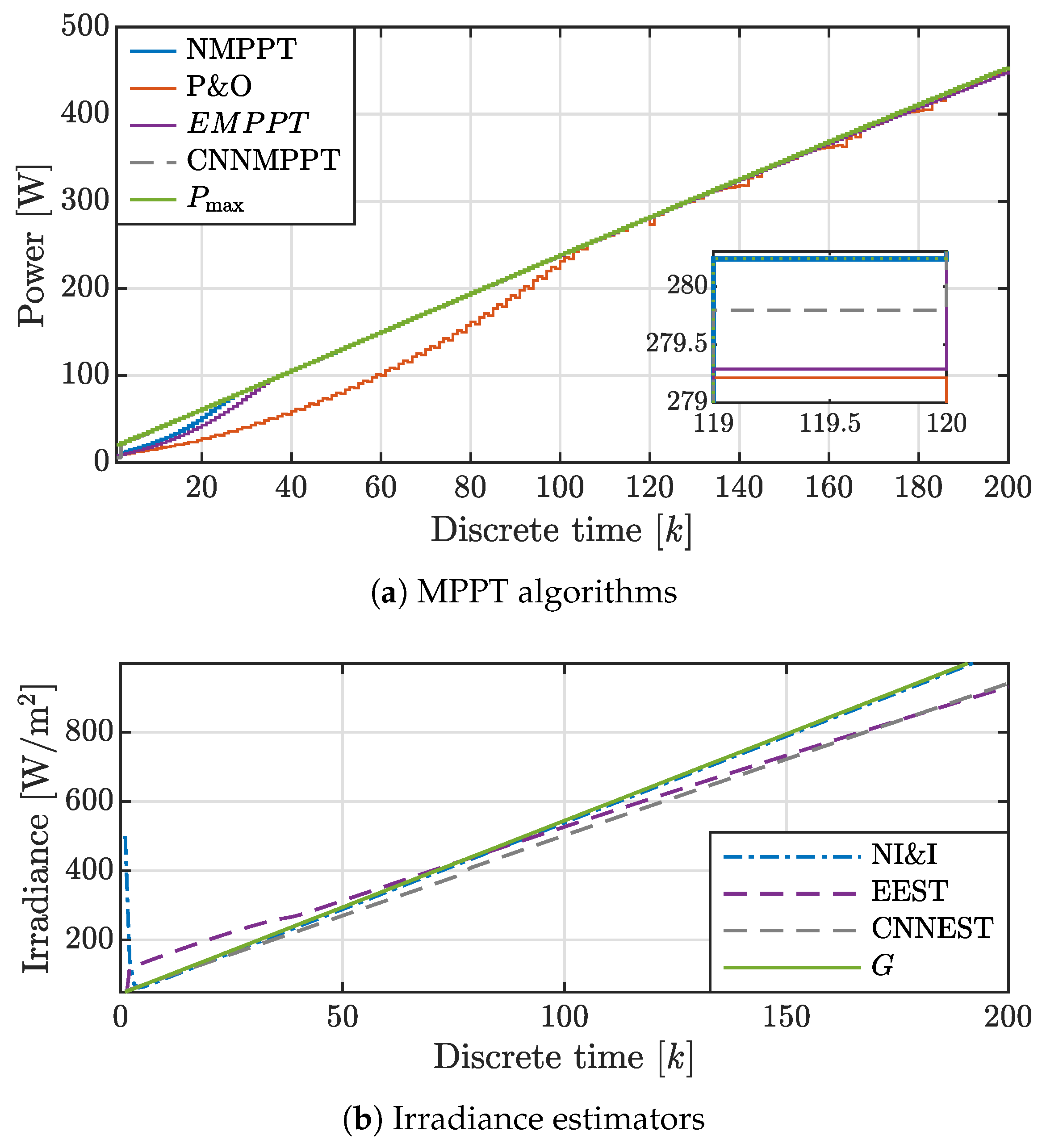
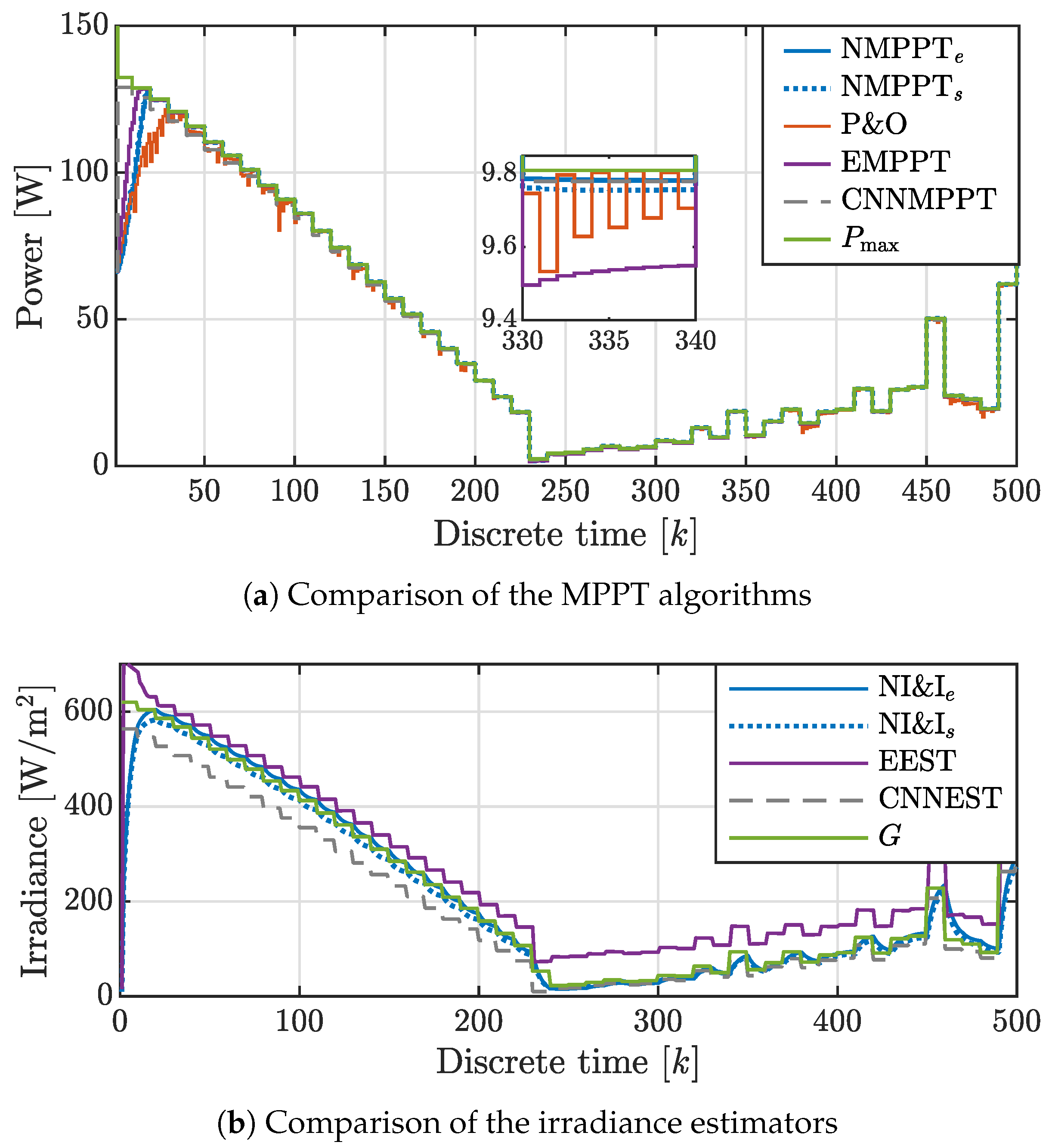
4. Simulation Results

The performance of the NMPPT algorithm is compared with the P&O [20] and CNNMPPT algorithm [38], as well as with the recently proposed MPPT algorithm that is based on the PV equivalent circuit (EMPPT) [29]. The EMPPT algorithm uses the irradiance estimator which is referred to as the EEST [29], while the irradiance estimator in the CNNMPPT is reffered to as the CNNEST. In the first set of examples, we used the I-V curves generated by the PV equivalent circuit. The PV panel consists of two serially connected PV modules, whose parameters are: $I_L=5.447\mathrm{A},{\mathrm{I}}_0=4.839\times {10}^{-12}\mathrm{A},$$R_p=309.047\mathsf{\Omega }$, $R_s=0.566\mathsf{\Omega },V_t=1.807\mathrm{V}$. On the other hand, the second subsection is related to the use of the large I-V curve repository provided by the National Renewable Energy Laboratory (NREL) [45]. We selected the I-V curve dataset of the PV module defined by the NREL identifier: HIT05662. The HIT05662 is modeled by the same equivalent circuit that is applied in the simulated examples. In all examples, the NN model consists of 4 neurons. The parameters in the P&O and EMPTT are chosen so that they provide the best performance. To ensure a fair comparison, the number of neurons in the CNNMPPT is set to 4. The parameters of the proposed method are $\mu =0.8,\gamma =50,\delta =1500$ in the first set of examples, and $\mu =1.5,\gamma =50$ in the second set of examples.

4.1. Simulated Data

The neural network is trained with 200 pairs of G and T, uniformly distributed within the ranges $G\in \{50,1100\}$ and $T\in \{5,50\}$. Each I-V curve consists of 100 operating points. Figure 6 shows the P-V curves of PV module and NN model for irradiance and temperature values which were not included in the training dataset. It can be seen that the P-V curves of the NN model coincide very well with those of the simulated model. The MSE for training data equals $2.92\times {10}^{-5}$, while the testing MSE is $3.81\times {10}^{-5}$.

In the first MPPT example, the performance of the proposed algorithm is assessed for different values of G. Precisely, during the first 30 iterations, the irradiance has value $G=900\mathrm{W}/{\mathrm{m}}^2$, after which it is changed to $G=600\mathrm{W}/{\mathrm{m}}^2$. In the first scenario, the NI&I algorithm is applied for the irradiance estimation. It may be observed from Figure 7b that the NI&I estimator converges in 15 iterations for $P=1$. On the other hand, the convergence speed of both the NI&I and NMPPT algorithm is increased as P reaches higher values (Figure 7a). In the second scenario, the gradient irradiance estimator is coupled with the NMPPT algorithm. It can be seen from Figure 7b that the NGE has faster convergence speed than the NI&I, which, additionally, causes the slightly faster convergence speed of the NMPPT algorithm. Considering the trade-off between the computational complexity and performance, in the remaining analysis, we used the NMPPT and NI&I estimator for $P=2$.

The second MPPT example describes the comparison between the NMPPT, P&O, EMPPT and CNNMMPT algorithm. Until the 100th iteration, the irradiance and the temperature are $G=320\mathrm{W}/{\mathrm{m}}^2$ and $T=10{}^{\circ }\mathrm{C}$, when they change to the values $G=725\mathrm{W}/{\mathrm{m}}^2$ and $T=50{}^{\circ }\mathrm{C}$. Observe from Figure 8a that the CNNMMPT provides the optimal voltage instantaneously, while the NMPPT, EMPPT and P&O algorithm need 8, 20 and 75 iterations to reach the steady-state, respectively. On the other hand, the NMPPT exhibits the smallest steady-state error, without oscillations. The reason for this is that the NI&I has greater accuracy than the EEST and CNNEST irradiance estimators, as can be seen from Figure 8b. Finally, in the P&O, the operating point oscillates about the MPP.

In the last example, the irradiance and the temperature are linearly changed within the ranges $G\in \{50,1050\}$, and $T\in \{5,55\}$. By observing the Figure 9a, it is possible to note that the NMPPT, EMPPT and CNNMPPT exhibit good tracking ability. The P&O has the slowest convergence speed, while the EMPPT has the largest steady-state error. It also can be seen that the NI&I estimator tracks the irradiance with the smaller error than the EEST and CNNEST (Figure 9b). The relative error between the predicted and true maximal power is shown in

Table 1. Relative error between the predicted and true maximal power.

k	G	${\mathit{P}}_{\mathit{max}}$	Prediction Error (%)
			NMPPT	P&O	EMPPT	CNNMPT
20	140	59.429	18.881	32.397	56.772	0.251
40	240	103.593	0.004	0.011	46.72	0.003
60	340	147.954	0.002	0.089	31.677	0.084
80	440	192.26	0.001	0.148	18.353	0.148
100	540	236.382	0.0001	0.224	6.007	0.171
120	640	280.24	0.001	0.339	0.366	0.159
140	740	323.775	0.0001	0.485	2.118	0.124
160	840	366.95	0.001	0.668	1.509	0.079
180	940	409.733	0.0001	0.885	1.708	0.036
200	1040	452.106	0.001	1.138	1.004	0.008

. Observe that, after the convergence, the proposed algorithm tracks the maximal power point with error less than $0.001\%$. Note also that in the EMPPT, P&O and CNNMMPT the relative error reaches the values 1.138%, 2.118% and 0.171%, respectively.

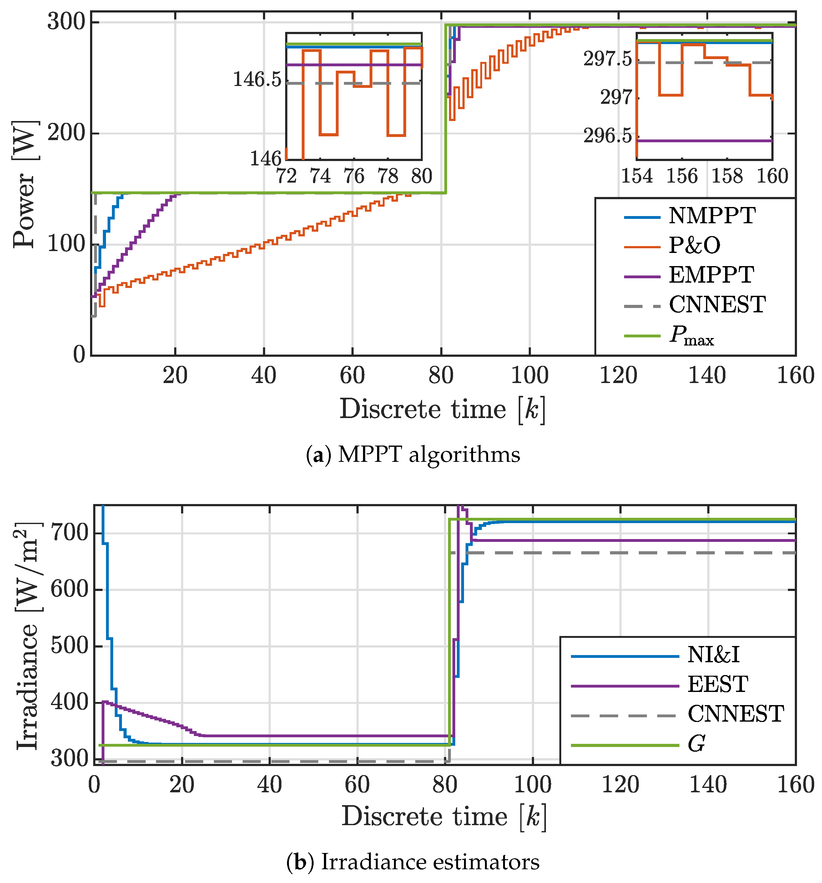
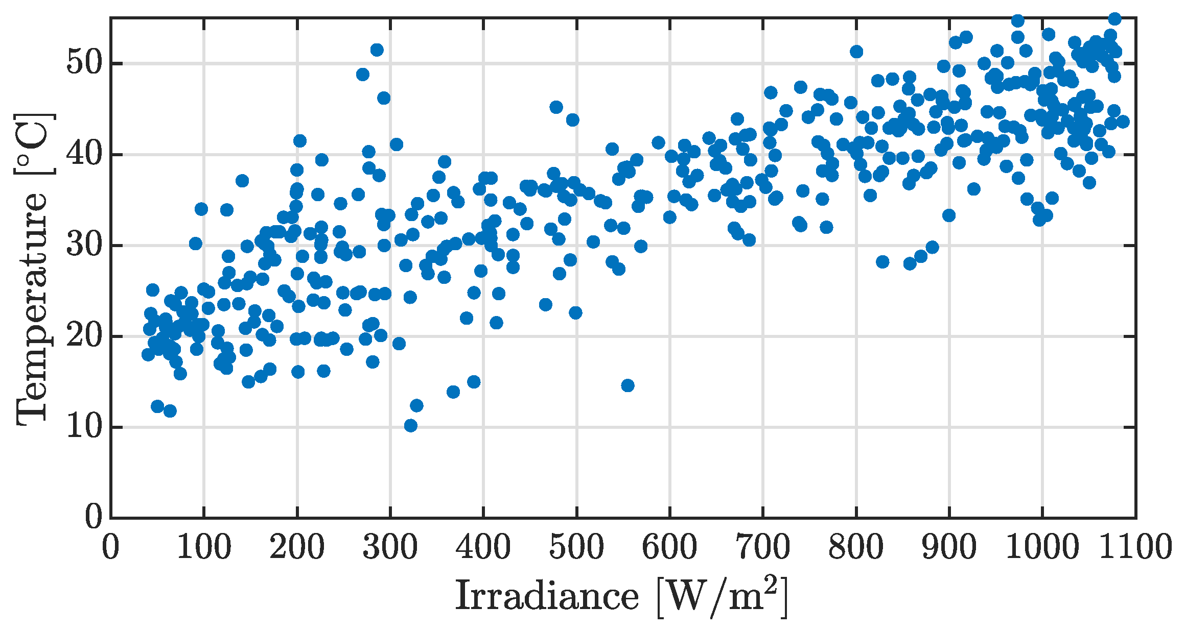
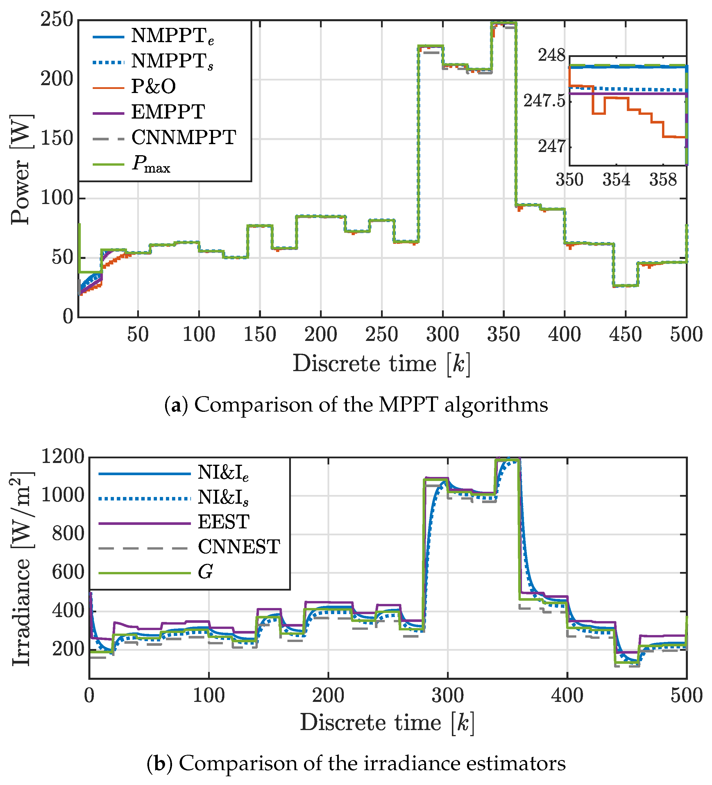
4.2. Experimental Data

The NN is trained for 500 different values of G and T, distributed in the ranges $\{50,1100\}$ and $\{5,50\}$, respectively (Figure 10). Each I-V curve contains 180 operating points. Figure 11 represents the P-V curves for values of irradiance and temperature which were not included in the training dataset. The subscripts e and s denote the NN models/NMPPT algorithms trained by experimental/simulated data, respectively. It can be seen that the P-V curves of the NN${}_e$ model coincide very well with the measured curves. The MSE for training data equals $0.0027$, while the testing MSE is $0.0028$. On the other hand, the MSE between the current generated by the NN${}_s$ model and measured current equals 0.0612.

In the first example, we performed a comparison between the considered algorithms under a sudden change in irradiance and temperature. Until the 100th iteration, the irradiance and the temperature are $G=320\mathrm{W}/{\mathrm{m}}^2$ and $T=10{}^{\circ }\mathrm{C}$, when they change to the values $G=725\mathrm{W}/{\mathrm{m}}^2$ and $T=50{}^{\circ }\mathrm{C}$. It can be perceived from Figure 12a that the CNNMMPT provides the optimal voltage instantaneously, while the NMPPT${}_e$, NMPPT${}_s$, EMPPT and P&O algorithm need 20, 23, 40 and 75 iterations to reach the steady-state, respectively. Note also that the NMPPT${}_e$ has the smallest steady-state error, followed by the NMPPT${}_s$, EMPPT, P&O and CNNMPPT. This behavior can be explained by the fact that EEST and NNEST have lower accuracy, which can be observed from Figure 12b.

Eventually, the last example focuses on the two time-varying irradiance and temperature profiles. Corresponding simulation results are presented in Figure 13 and Figure 14. A similar conclusion as in the previous example can be drawn here. The NMPPT algorithm and NI&I estimator, which are based on the experimental data, provide the best steady-state performance. On the other hand, both the NMPPT${}_s$ and EMPPT exhibit acceptable performance. It can also be seen that the NI&I${}_s$ has greater accuracy than the EEST and NNEST. The P&O algorithm has the slowest tracking speed and exhibits oscillations in the steady-state. Finally, the CNNMPT for some irradiance levels has good accuracy, while for some irradiance levels exhibits the worst performance. The relative error between the predicted and true maximal power for different irradiance level is shown in

Table 2. Relative error between the predicted and true maximal power.

G	${\mathit{P}}_{\mathit{max}}$	Prediction Error (%)
		NMPPT${}_{\mathit{e}}$	NMPPT${}_{\mathit{s}}$	EMPPT	P&O	CNNMPT
110.2	22.77	0.06	0.082	0.408	1.856	1.834
132.2	23.635	0.099	0.064	0.218	0.187	0.712
225.1	46.391	0.003	0.012	0.097	0.11	0.177
260.5	54.285	0.007	0.007	0.058	0.321	0.536
302.9	61.845	0.004	0.012	0.046	0.117	0.537
369.9	77.121	0.01	0.002	0.023	0.291	0.333
409.7	84.877	0.001	0.001	0.005	0.24	0.43
523.5	111.36	0.009	0.051	0.064	0.6328	0.016
613.3	120.578	0.006	0.267	0.023	0.027	0.04
653.8	133.64	0.007	0.01	0.016	1.746	0.046
713.40	153.97	0.0004	0.2259	0.2473	0.2680	0.9709
859.5	171.037	0.0001	0.005	0.002	0.006	0.262
946.8	198.125	0.001	0.142	0.163	0.72	0.572
1007.1	208.772	0.004	0.06	0.07	0.123	1.581
1084.3	228.473	0.003	0.173	0.118	0.209	2.586

. Observe that the NMPPT${}_e$ tracks the maximal power point with error less than $0.1\%$. Note also that in the NMPPT${}_s$, EMPPT, P&O and CNNMMPT the relative error reaches the values 0.2259%, 0.408%, 1.856% and 2.586%, respectively.

5. Conclusions

In this paper, the simple and accurate gradient MPPT algorithm based on the neural network model of the photovoltaic module has been proposed. The NN model is utilized to calculate the gradient of the P-V curve with respect to the voltage, which enables fast tracking of the MPP and steady-state performance without oscillations. Additionally, the irradiance estimator, which also relies on the NN model, has been presented. It is important to emphasize that the NN model can be developed either by using the experimental data or the data generated by the equivalent circuit model.

Suitable simulations have been performed for comparing our approach with the effective techniques proposed in the literature. The final results indicate that the proposed MPPT algorithm exhibits faster convergence speed compared to the other iterative algorithms. It has been also demonstrated that the experimental-data-based NN model achieves the best steady-state performance, as well as that the acceptable performance can be obtained with the simulated-data-based NN model. Furthermore, the proposed irradiance estimator exhibits greater or similar accuracy compared to the considered algorithms. This is also of great importance since the irradiance estimators can be used for other purposes such as monitoring and fault detection of PV systems. Lastly, the proposed approach does not only achieve high degrees of accuracy, but it also has low computation complexity, which makes it suitable for implementation on microprocessor platforms.

References

1. Laudani, A.; Mancilla-David, F.; Riganti-Fulginei, F.; Salvini, A. Reduced-form of the photovoltaic five-parameter model for efficient computation of parameters. Sol. Energy 2013, 97, 122–127. [Google Scholar] [CrossRef]
2. Mahmoud, Y.; El-Saadany, E.F. Photovoltaic model with reduced computational time. IEEE Trans. Ind. Electron. 2015, 62, 3534–3544. [Google Scholar] [CrossRef]
3. Chin, V.J.; Salam, Z.; Ishaque, K. An Accurate and fast computational algorithm for the two-diode model of PV module based on a hybrid method. IEEE Trans. Ind. Electron. 2017, 64, 6212–6222. [Google Scholar] [CrossRef]
4. Stornelli, V.; Muttillo, M.; de Rubeis, T.; Nardi, I. A New Simplified Five-Parameter Estimation Method for Single-Diode Model of Photovoltaic Panels. Energies 2019, 12, 4271. [Google Scholar] [CrossRef] [Green Version]
5. Laudani, A.; Riganti Fulginei, F.; Salvini, A. High performing extraction procedure for the one-diode model of a photovoltaic panel from experimental I-V curves by using reduced forms. Sol. Energy 2014, 103, 316–326. [Google Scholar] [CrossRef]
6. Kang, T.; Yao, J.; Jin, M.; Yang, S.; Duong, T. A Novel Improved Cuckoo Search Algorithm for Parameter Estimation of Photovoltaic (PV) Models. Energies 2018, 11, 1060. [Google Scholar] [CrossRef] [Green Version]
7. Javier Toledo, F.; Blanes, J.M.; Galiano, V. Two-Step Linear Least-Squares Method for Photovoltaic Single-Diode Model Parameters Extraction. IEEE Trans. Ind. Electron. 2018, 65, 6301–6308. [Google Scholar] [CrossRef]
8. Huang, P.H.; Xiao, W.; Peng, J.C.; Kirtley, J.L. Comprehensive Parameterization of Solar Cell: Improved Accuracy with Simulation Efficiency. IEEE Trans. Ind. Electron. 2016, 63, 1549–1560. [Google Scholar] [CrossRef]
9. Jain, A.; Sharma, S.; Kapoor, A. Solar cell array parameters using Lambert W-function. Sol. Energy Mater. Sol. Cells 2006, 90, 25–31. [Google Scholar] [CrossRef]
10. Batzelis, E.I.; Routsolias, I.A.; Papathanassiou, S.A. An explicit pv string model based on the lambert w function and simplified mpp expressions for operation under partial shading. IEEE Trans. Sustain. Energy 2014, 5, 301–312. [Google Scholar] [CrossRef]
11. Almonacid, F.; Fernandez, E.F.; Mellit, A.; Kalogirou, S. Review of techniques based on artificial neural networks for the electrical characterization of concentrator photovoltaic technology. Renew. Sustain. Energy Rev. 2017, 75, 938–953. [Google Scholar] [CrossRef]
12. Castro, R. Data-driven PV modules modelling: Comparison between equivalent electric circuit and artificial intelligence based models. Sustain. Energy Technol. Assess. 2018, 30, 230–238. [Google Scholar] [CrossRef]
13. Xu, X.; Zhang, X.; Huang, Z.; Xie, S.; Gu, W.; Wang, X.; Zhang, L.; Zhang, Z. Current Characteristics Estimation of Si PV Modules Based on Artificial Neural Network Modeling. Materials 2019, 12, 3037. [Google Scholar] [CrossRef] [PubMed] [Green Version]
14. Khatib, T.; Ghareeb, A.; Tamimi, M.; Jaber, M.; Jaradat, S. A new offline method for extracting I-V characteristic curve for photovoltaic modules using artificial neural networks. Sol. Energy 2018, 173, 462–469. [Google Scholar] [CrossRef]
15. Bonanno, F.; Capizzi, G.; Graditi, G.; Napoli, C.; Tina, G.M. A radial basis function neural network based approach for the electrical characteristics estimation of a photovoltaic module. Appl. Energy 2012, 97, 956–961. [Google Scholar] [CrossRef] [Green Version]
16. Chen, Z.; Chen, Y.; Wu, L.; Cheng, S.; Lin, P.; You, L. Accurate modeling of photovoltaic modules using a 1-D deep residual network based on I-V characteristics. Energy Convers. Manag. 2019, 186, 168–187. [Google Scholar] [CrossRef]
17. Ma, X.; Huang, W.H.; Schnabel, E.; Kohl, M.; Brynjarsdottir, J.; Braid, J.L.; French, R.H. Data-Driven $I$$V$ Feature Extraction for Photovoltaic Modules. IEEE J. Photovolt. 2019, 9, 1405–1412. [Google Scholar] [CrossRef] [Green Version]
18. Chikh, A.; Chandra, A. Adaptive neuro-fuzzy based solar cell model. IET Renew. Power Gener. 2014, 8, 679–686. [Google Scholar] [CrossRef]
19. Mahmod Mohammad, A.N.; Mohd Radzi, M.A.; Azis, N.; Shafie, S.; Atiqi Mohd Zainuri, M.A. An Enhanced Adaptive Perturb and Observe Technique for Efficient Maximum Power Point Tracking Under Partial Shading Conditions. Appl. Sci. 2020, 10, 3912. [Google Scholar] [CrossRef]
20. Kapić, A.; Zečević, Ž.; Krstajić, B. An efficient MPPT algorithm for PV modules under partial shading and sudden change in irradiance. In Proceedings of the 2018 23rd International Scientific-Professional Conference on Information Technology (IT), Zabljak, Montenegro, 19–24 February 2018; pp. 1–4. [Google Scholar] [CrossRef]
21. Erauskin, R.L.; Gonzalez, A.; Petrone, G.; Spagnuolo, G.; Gyselinck, J. Multi-Variable Perturb & Observe Algorithm for Grid-tied PV Systems with Joint Central and Distributed MPPT Configuration. IEEE Trans. Sustain. Energy 2020. [Google Scholar] [CrossRef]
22. Bhattacharyya, S.; Patnam, D.S.K.; Samanta, S.; Mishra, S. Steady Output and Fast Tracking MPPT (SOFT MPPT) for P&O and InC Algorithms. IEEE Trans. Sustain. Energy 2020. [Google Scholar] [CrossRef]
23. Zakzouk, N.E.; Elsaharty, M.A.; Abdelsalam, A.K.; Helal, A.A.; Williams, B.W. Improved performance low-cost incremental conductance PV MPPT technique. IET Renew. Power Gener. 2016, 10, 561–574. [Google Scholar] [CrossRef] [Green Version]
24. Alsumiri, M. Residual Incremental Conductance Based Nonparametric MPPT Control for Solar Photovoltaic Energy Conversion System. IEEE Access 2019, 7, 87901–87906. [Google Scholar] [CrossRef]
25. Dolara, A.; Grimaccia, F.; Mussetta, M.; Ogliari, E.; Leva, S. An Evolutionary-Based MPPT Algorithm for Photovoltaic Systems under Dynamic Partial Shading. Appl. Sci. 2018, 8, 558. [Google Scholar] [CrossRef] [Green Version]
26. Li, W.; Zhang, G.; Pan, T.; Zhang, Z.; Geng, Y.; Wang, J. A Lipschitz Optimization-Based MPPT Algorithm for Photovoltaic System under Partial Shading Condition. IEEE Access 2019, 7, 126323–126333. [Google Scholar] [CrossRef]
27. Ali, A.; Almutairi, K.; Malik, M.Z.; Irshad, K.; Tirth, V.; Algarni, S.; Zahir, M.H.; Islam, S.; Shafiullah, M.; Shukla, N.K. Review of Online and Soft Computing Maximum Power Point Tracking Techniques under Non-Uniform Solar Irradiation Conditions. Energies 2020, 13, 3256. [Google Scholar] [CrossRef]
28. Mahmoud, Y.; Abdelwahed, M.; El-Saadany, E.F. An Enhanced MPPT Method Combining Model-Based and Heuristic Techniques. IEEE Trans. Sustain. Energy 2016, 7, 576–585. [Google Scholar] [CrossRef]
29. Moshksar, E.; Ghanbari, T. A model-based algorithm for maximum power point tracking of PV systems using exact analytical solution of single-diode equivalent model. Sol. Energy 2018, 162, 117–131. [Google Scholar] [CrossRef]
30. Elobaid, L.M.; Abdelsalam, A.K.; Zakzouk, E.E. Artificial neural network-based photovoltaic maximum power point tracking techniques: A survey. IET Renew. Power Gener. 2015, 9, 1043–1063. [Google Scholar] [CrossRef]
31. Hiyama, T.; Kouzuma, S.; Imakubo, T.; Ortmeyer, T.H. Evaluation of Neural Network Based Real Time Maximum Power Tracking Controller for PV System. IEEE Trans. Energy Convers. 1995, 10, 543–548. [Google Scholar] [CrossRef]
32. Ocran, T.A.; Cao, J.; Cao, B.; Sun, X. Artificial neural network maximum power point tracker for solar electric vehicle. Tsinghua Sci. Technol. 2005, 10, 204–208. [Google Scholar] [CrossRef]
33. Gowid, S.; Massoud, A. A robust experimental-based artificial neural network approach for photovoltaic maximum power point identification considering electrical, thermal and meteorological impact. Alex. Eng. J. 2020. [Google Scholar] [CrossRef]
34. Sedaghati, F.; Nahavandi, A.; Badamchizadeh, M.A.; Ghaemi, S.; Abedinpour Fallah, M. PV maximum power-point tracking by using artificial neural network. Math. Probl. Eng. 2012, 2012. [Google Scholar] [CrossRef]
35. Essefi, R.M.; Souissi, M.; Abdallah, H.H. Maximum Power Point Tracking Control Using Neural Networks for Stand-Alone Photovoltaic Systems. Int. J. Mod. Nonlinear Theory Appl. 2014, 3, 53–65. [Google Scholar] [CrossRef] [Green Version]
36. Rolevski, M.; Zecevic, Z. MPPT controller based on the neural network model of the photovoltaic panel. In Proceedings of the 2020 24th International Conference on Information Technology (IT), Zabljak, Montenegro, 18–22 February 2020; pp. 1–4. [Google Scholar] [CrossRef]
37. Rizzo, S.A.; Scelba, G. ANN based MPPT method for rapidly variable shading conditions. Appl. Energy 2015, 145, 124–132. [Google Scholar] [CrossRef]
38. Elobaid, L.M.; Abdelsalam, A.K.; Zakzouk, E.E. Artificial neural network based maximum power point tracking technique for PV systems. In Proceedings of the IECON 2012—38th Annual Conference on IEEE Industrial Electronics Society, Montreal, QC, Canada, 25–28 October 2012; pp. 937–942. [Google Scholar] [CrossRef]
39. Chikh, A.; Chandra, A. An Optimal Maximum Power Point Tracking Algorithm for PV Systems with Climatic Parameters Estimation. IEEE Trans. Sustain. Energy 2015, 6, 644–652. [Google Scholar] [CrossRef]
40. Mancilla-David, F.; Riganti-Fulginei, F.; Laudani, A.; Salvini, A. A Neural Network-Based Low-Cost Solar Irradiance Sensor. IEEE Trans. Instrum. Meas. 2014, 63, 583–591. [Google Scholar] [CrossRef]
41. Carrasco, M.; Mancilla-David, F.; Ortega, R. An estimator of solar irradiance in photovoltaic arrays with guaranteed stability properties. IEEE Trans. Ind. Electron. 2014, 61, 3359–3366. [Google Scholar] [CrossRef]
42. Yilmaz, U.; Turksoy, O.; Teke, A. Improved MPPT method to increase accuracy and speed in photovoltaic systems under variable atmospheric conditions. Int. J. Electr. Power Energy Syst. 2019, 113, 634–651. [Google Scholar] [CrossRef]
43. Bendib, B.; Krim, F.; Belmili, H.; Almi, M.F.; Bolouma, S. An intelligent MPPT approach based on neural-network voltage estimator and fuzzy controller, applied to a stand-alone PV system. In Proceedings of the 2014 IEEE 23rd International Symposium on Industrial Electronics (ISIE), Istanbul, Turkey, 1–4 June 2014; pp. 404–409. [Google Scholar] [CrossRef]
44. Çelik, Ö.; Teke, A. A Hybrid MPPT method for grid connected photovoltaic systems under rapidly changing atmospheric conditions. Electr. Power Syst. Res. 2017, 152, 194–210. [Google Scholar] [CrossRef]
45. Marion, B.; Anderberg, A.; Deline, C.; del Cueto, J.; Muller, M.; Perrin, G.; Rodriguez, J.; Rummel, S.; Silverman, T.J.; Vignola, F.; et al. New data set for validating PV module performance models. In Proceedings of the 2014 IEEE 40th Photovoltaic Specialist Conference (PVSC), Denver, CO, USA, 8–13 June 2014; pp. 1362–1366. [Google Scholar] [CrossRef]
Figure 1. Equivalent electrical circuit of a PV module.
Applsci 10 05051 g001
Figure 2. P-V curve for different values of irradiance and temperature.
Applsci 10 05051 g002
Figure 3. The architecture of neural network model of the PV.
Applsci 10 05051 g003
Figure 4. Schematic arrangement for the PV system.
Applsci 10 05051 g004
Figure 5. The architecture of the neural networks used for MPP voltage and irradiance estimation.
Applsci 10 05051 g005
Figure 6. Comparison between P-V curves of PV module generated by the equivalent circuit and NN model of the photovoltaic.
Applsci 10 05051 g006
Figure 7. Performance of the proposed algorithm for different values of P.
Applsci 10 05051 g007
Figure 8. Comparison of the algorithms under sudden change in irradiance.
Applsci 10 05051 g008
Figure 9. Comparison of the algorithms under linearly varying irradiance and temperature.
Applsci 10 05051 g009
Figure 10. The experimental data used for the training of the NMPPT.
Applsci 10 05051 g010
Figure 11. Comparison between measured P-V curves and P-V curves generated by NN models.
Applsci 10 05051 g011
Figure 12. Comparison of the algorithms under sudden change in irradiance.
Applsci 10 05051 g012
Figure 13. Comparison of the algorithms under time varying profile of the solar irradiance.
Applsci 10 05051 g013
Figure 14. Comparison of the algorithms under time varying profile of the solar irradiance.
Applsci 10 05051 g014