Article

Off-Design Performance Prediction of a S-CO2 Turbine Based on Field Reconstruction Using Deep-Learning Approach

State Key Laboratory for Strength and Vibration of Mechanical Structures, School of Energy and Power Engineering, Xi’an Jiaotong University, Xi’an 710049, China
*
Author to whom correspondence should be addressed.
Appl. Sci. 2020, 10(14), 4999; https://doi.org/10.3390/app10144999
Submission received: 18 June 2020 / Revised: 15 July 2020 / Accepted: 16 July 2020 / Published: 21 July 2020
(This article belongs to the Section Energy Science and Technology)

Abstract

:

Featured Application

In this research, a two-stage deep convolutional neural network is proposed to predict the off-design performance of a S-CO2 turbine based on field reconstruction. Once the deep model is well-trained, the calculation with graphics processing unit (GPU)-acceleration can quickly predict the physical fields on the blade surface and turbine performance. In practical engineering applications, the proposed method can not only reduce the design cycle of components but also help to grasp the actual operating conditions in real time.

Abstract

The reliable design of the supercritical carbon dioxide (S-CO2) turbine is the core of the advanced S-CO2 power generation technology. However, the traditional computational fluid dynamics (CFD) method is usually applied in the S-CO2 turbine design-optimization, which is a high computational cost, high memory requirement, and long time-consuming solver. In this research, a flexible end-to-end deep learning approach is presented for the off-design performance prediction of the S-CO2 turbine based on physical fields reconstruction. Our approach consists of three steps: firstly, an optimal design of a 60,000 rpm S-CO2 turbine is established. Secondly, five design variables for off-design analysis are selected to reconstruct the temperature and pressure fields on the blade surface through a deconvolutional neural network. Finally, the power and efficiency of the turbine is predicted by a convolutional neural network according to reconstruction fields. The results show that the prediction approach not only outperforms five classical machine learning models but also focused on the physical mechanism of turbine design. In addition, once the deep model is well-trained, the calculation with graphics processing unit (GPU)-accelerated can quickly predict the physical fields and performance. This prediction approach requires less human intervention and has the advantages of being universal, flexible, and easy to implement.

1. Introduction

Supercritical carbon dioxide (S-CO2) refers to the carbon dioxide fluid above the critical point (30.98 °C, 7.38 MPa) [1]. It has the advantages of being stable chemical properties, weak high-temperature corrosion, non-toxic, and non-combustible. At the same time, it has the characteristics of high specific heat capacity and density, high thermal conductivity, and low viscosity. S-CO2 is an ideal low-cost working medium [2,3]. Therefore, a Brayton power generation system with S-CO2 has the advantages of high-efficiency, small-volume, and low-noise (mainly high-frequency noise). It has become one of the main research directions in the field of power generation technology (nuclear energy, solar energy, geothermal energy, waste heat, etc.) [4,5,6,7].
Turbine is the “heart” of the whole power cycle. The power and efficiency of the system are directly affected by its performance. Therefore, the research on S-CO2 turbine has become a hot spot. Sandia National Laboratory [8] developed a 100 kW centripetal turbine and a 50 kW centrifugal compressor, and conducted a large number of S-CO2 closed cycle tests from 2007 to 2009. A labyrinth seal turbine wheel was developed by Korea Institute of Energy Research [9]. It was applied to a 10 kW S-CO2 Brayton experimental loop. Zhou et al. [10] proposed a design method of S-CO2 radial turbine. The one-dimensional (1-D) model and three-dimensional (3-D) numerical simulation methods were adopted to predict the off-design performance. Han et al. [11] completed the design of high-pressure and low-pressure axial-flow turbines applied to 5 MW S-CO2 reheated Brayton cycle by using the self-designed program. The isentropic efficiencies of the turbines were 82.88% and 82.26%, respectively. A 10 MW S-CO2 single stage centrifugal turbine was designed and numerically analyzed by Luo et al. [12]. The total-static efficiency after blade shape optimization was 89.02%. At present, computational fluid dynamics (CFD) is still the main method of turbine aerodynamic design and analysis. However, a lot of iterative calculations are needed to solve the Navier–Stokes (NS) equation. This is time-consuming and expensive to calculate. It also delays the entire design and analysis cycle. Therefore, it is necessary to develop a more efficient and accurate method than CFD.
With the development of computers, CFD method is widely used. Hence, a large number of CFD data are generated in the process of design and optimization. Therefore, the data-based proxy model becomes more and more practical and important. Previous studies have shown that when the machine learning algorithm is properly selected and fully utilized, surrogate models based on that can well predict the performance of components in power cycle. Based on Levenberg–Marquardt algorithm, Yu et al. [13] proposed a back-propagation neural network to predict the off-design or overall dynamic performance of the gas turbine. Rossi and Renzi [14] developed a computational methodology based on artificial neural networks (ANNs). It could accurately predict the performance-curve and best-efficiency-point of turbo pump working in reverse mode. This proved that ANNs are a universal and effective evaluation tool. Based on neural network surrogate models, Palagi et al. [15] proposed an optimization model for main design parameters of the radial turbine. The designed neural networks had high accuracy and could accurately learn highly nonlinear physical model objects. Sarafraz et al. [16,17,18] developed the response surface methodology (RSM) for the optimization of a catalytic reforming micro-reactor and a thermosyphon heat pipe. The above examples have shown that machine learning can be used for component performance prediction, but such surrogate models belong to the black-box model, ignoring the physical relationship between parameters, and have little effect on grasping the operation rules of components and guiding component control.
In recent years, some scholars have reconstructed similar heat transfer or mass transfer problems based on the rapidly developing deep learning algorithm, aiming to obtain a surrogate model that can consider the physical mechanism. Guo et al. [19] adopted a convolutional neural network (CNN) to the prediction of the velocity field with different geometric shapes, while convolution and deconvolution operations were used to perform image-to-image regression. Although the accuracy rate reached 98%, there were prediction errors near the boundary. Based on the deep convolutional neural network, the Cp-u model was proposed by Jin et al. [20] for the prediction of the unsteady velocity around a circular cylinder. Compared with the measured data, it had good accuracy. Ti et al. [21] proposed an innovative framework based on the machine learning and CFD simulation to improve the prediction accuracy of turbine wake. The results of the turbine wake model based on ANN were in good agreement with the numerical and experimental data, which showed that the ANN can establish the complex spatial relationship of the problem. In summary, deep learning has been used in the reconstruction of problems such as velocity field, pressure field, and temperature field, and has shown high accuracy and performance.
Based on the above introduction, it can be found that there are two main methods to predict the performance of components in power cycles, especially S-CO2 turbines: the mechanism-based physical model and the data-based proxy model. The mechanism-based physical model is a conventional CFD solution method. It mainly solves NS equations on computational grids with corresponding boundary conditions. Although this method is accurate, the time and cost of calculation are very high. The performance prediction of related components shows high prediction efficiency and accuracy. However, it cannot capture the details of heat and mass transfer process in turbine. However, in solutions to similar problems, deep learning can overcome the above shortcomings. Therefore, in order to improve the accuracy and efficiency of performance prediction while preserving the physical field information, a performance prediction method of S-CO2 turbines based on CNN is proposed.
Our contributions are as follows:
  • The performance of field reconstruction for an end-to-end deep learning method is explored in this research. The most existing machine learning methods only focus on one target variable in engineering design and optimization tasks. The fields predicted by our method can provide more flow mechanism explanations and help designers understand the physical process.
  • The data-based proxy model is established for a physical system. Traditional methods lack accuracy to some extent and require manual intervention. Based on the existing scientific database, this method does not need to rely on human intervention and has the advantages of being universal, flexible, and easy to implement, showing a good promise for real-time control and design optimization of turbines.
  • The method proposed in this research is effective and accurate. The off-design power and efficiency prediction in this method is able to reach performance comparable to a state-of-the-art model and clearly outperforms classical methods. In addition, once the deep model is well-trained, the calculation with GPU-accelerated can quickly predict the physical fields on the blade surface and turbine performance.
This flexible and adaptive tool can not only reduce the design cycle of turbine components, but also help to grasp the actual operating conditions in real time, which can be applied to adjust and control the system in time.
The rest of this paper is organized as below: Section 2 introduces the overall architecture of this research, the theory and method of CFD analysis and deep convolutional neural network; Section 3 is the results and discussion, including CFD off-design pre-analysis, flow field reconstruction, and performance prediction. Section 4 draws conclusions.

2. Theory and Method

2.1. Overall Architecture

In this research, the end-to-end reconstruction deep convolutional neural network implemented by deep learning framework Pytorch [22] was utilized to reconstruct the expand process in the S-CO2 turbine based on main design parameters and then predict the aerodynamic performance of S-CO2 turbine from reconstructed results.
As illustrated in Figure 1, the proposed end-to-end framework includes three stages. The stage 0 was applied to obtain real field structures and performance of the designed S-CO2 turbine from numerical results in the off-design analysis. In the next two stages, a deep convolutional neural network was employed to reconstruct interested physical fields and predict turbine performance based on physical fields. At stage 1, the interested physical fields were reconstructed with design variables including geometric variables and environmental condition variables as input. Subsequently, the performance of the S-CO2 turbine was predicted at stage 2. It should be noted that the input of performance prediction model can be the reconstructed fields from stage 1 or the real fields from off-design analysis.

2.2. CFD Analysis Method

The general forms of the three control equations mass conservation equation, momentum conservation equation, and energy conservation equation can be expressed as follows [23,24]:
( ρ ϕ ) t + div ( ρ U ϕ ) = div ( Γ ϕ grad ϕ ) + S ϕ
where ρ is density, t is time, U is velocity, Γ ϕ is the generalized diffusion coefficient, S ϕ is the generalized source term, and ϕ is the general variable.
In this study, the zonal shear stress transport (SST) k ω turbulence model was adopted. It was raised by Menter [25] on the basis of standard k ω turbulence model. This turbulence model is considered by more and more scholars as the preferred choice in the field of fluid machinery. Additionally, it has a good agreement with measurement data [26,27]. The transport equation is:
( ρ k ) t + ( ρ k u i ¯ ) x i = x j [ Γ k k x j ] + G k Y k
( ρ ω ) t + ( ρ ω u j ¯ ) x j = x j [ Γ ω ω x j ] + G ω Y ω + D ω
where u i ¯ and u j ¯ are the average turbulent velocity, x i and x j are the coordinate component, G k is the generation term of turbulent kinetic energy k based on the average velocity gradient, G ω is the generation term of dissipation rate ω , Y k is the dissipation term of k , Y ω is the dissipation term of ω , Γ k and Γ ω are the effective diffusion coefficients of k and ω , respectively, D ω is cross-diffusion term, which coordinates the interface between the standard k ε turbulence model and the standard k ω turbulence model.
The formula of turbulent dynamic viscosity coefficient μ t of the modified turbulence model is as follows:
μ t = ρ k ω 1 max [ 1 α * , c F 2 α 0 ω ]
where α * is the low Reynolds number correction coefficient for reducing turbulent eddy viscosity, c is the constant term of shear stress tensor, α 0 is the empirical constant, and F 2 is the mixed function.
Based on a large number of physical characteristics data of carbon dioxide, the explicit equation of Helmholtz energy equation, the improved Benedict Webb Rubin (MBWR) state equation and the extended corresponding state (ECS) model were adopted. The MBWR state equation is as follows:
P = n = 1 9 a n ρ n + exp ( ( ρ ρ c ) 2 ) n = 10 15 a n ρ 2 n 17
where P is pressure, ρ c is critical density, and a n is characteristic parameters related to temperature.
In this study, x = [ T i n , P i n , α 1 , m ˙ , ω R ] is taken as the design variable of the turbine, including: inlet temperature T i n , inlet pressure P i n , inlet air flow angle α 1 , mass flow rate m ˙ , and rotating speed ω R . The real result field f obtained by 3-D CFD analysis is as follows:
f = F cfd ( x ) = [ P , T ]
where P is pressure fields and T is the temperature fields.
According to 3-D numerical results, the pressure and temperature distribution on the blade surface can be obtained. Additionally, then the performance of turbine ψ , power p , and efficiency η can be calculated based on fields information:
ψ = F per ( f ) = [ p , η ]
The torque of the turbine TR is obtained by solving the torque difference on the rotor blade surface between pressure side and suction side by integral method. The formula of power is as follows:
p = T R ω R = [ ( r P d A ) ps ( r P d A ) ss ] ω R
where r is the radius, d A is the unit surface area, subscript ps is the rotor blade pressure surface and ss is the rotor blade suction surface.
The total static efficiency of the turbine is:
η T S = p m ˙ [ h ( P i n , T i n ) h ( S ( P i n , T i n ) , P o u t ) ]
where m ˙ is the mass flow (obtained by numerical simulation), h is the enthalpy, S is the entropy, the subscripts in and out, respectively, represent the turbine inlet and outlet.

2.3. Deep Convolutional Neural Network

In Figure 1, the architecture of the two-stage deep convolutional neural network composed by two stages, stage 1 employed as field reconstruction model and stage 2 employed as performance prediction model, is described in detail.
In stage 1, the field reconstruction model with deconvolutional neural network is trained by minimum the loss function s t a g e 1 between real and predicted fields. With the predicted fields from stage 1 as input, the performance prediction model with convolutional neural network is trained by minimum the loss function s t a g e 2 between real and predicted performance. It should be emphasized that the s t a g e 2 backward propagate through both the convolutional and deconvolutional neural networks if reconstructed fields are the input, while the s t a g e 2 just backpropagate through the convolutional neural network with real fields as input.
In stage 1, the deconvolutional neural network is employed to establish the reconstruction mapping from design variables. The input is design parameters x , while the temperature and pressure fields are target physical fields.
Assuming the reconstruction mapping in stage 1 can be defined as followed:
f ^ = F ^ 1 ( x ; Θ 1 )
where x is the input design variables, f ^ is the reconstructed field, Θ 1 is the learnable parameters in reconstruction deconvolutional neural network, the reconstruction mapping F ^ 1 can be obtained by minimizing the expectation of loss function s t a g e 1 in the definition domain of the dataset.
The training process of stage 1 is presented as:
Θ 1 = arg min Θ 1 E x , f D ( s t a g e 1 )
where { x , f } D indicates design variables and fields samples obtained by numerical simulations in definition domain D .
At stage 2, the performance is predicted from physical fields using a deep convolutional neural network. In this study, the input at stage 2 is the reconstructed fields obtained at stage 1 and the output is the interested performance of S-CO2 turbine, power, and efficiency. The mapping function from physical fields too performance can be described as follows:
ψ ^ = F ^ 2 ( f ^ ; Θ 2 ) = F ^ 2 ( F ^ 1 ( x ; Θ 1 ) ; Θ 2 )
where ψ ^ is the predicted turbine performance, f ^ is the reconstruction field at stage 1, Θ 2 is the learnable parameters of the deep convolutional neural network, the mapping function F ^ 2 can be obtained by minimizing the expectation of loss function s t a g e 2 in the definition domain of the dataset.
The training process of stage 2 is formalized as:
Θ 2 = arg min Θ 2 E f , ψ D ( s t a g e 2 )
where { f , ψ } D indicates fields and performance samples obtained by numerical simulations in definition domain D .
It is obvious that the input design variables of stage 1 are low dimensional data while the physical fields with high dimension are obtained as output. Thus, deconvolutional neural network is utilized to expand low-dimensional input to high-dimensional fields. Deconvolutional neural network was first proposed by Zelier [28] and the general application was presented in their following works [29,30]. With the development of deconvolutional neural network, plenty of applications are conducted on scene segmentation [31], image processing [32], and so on.
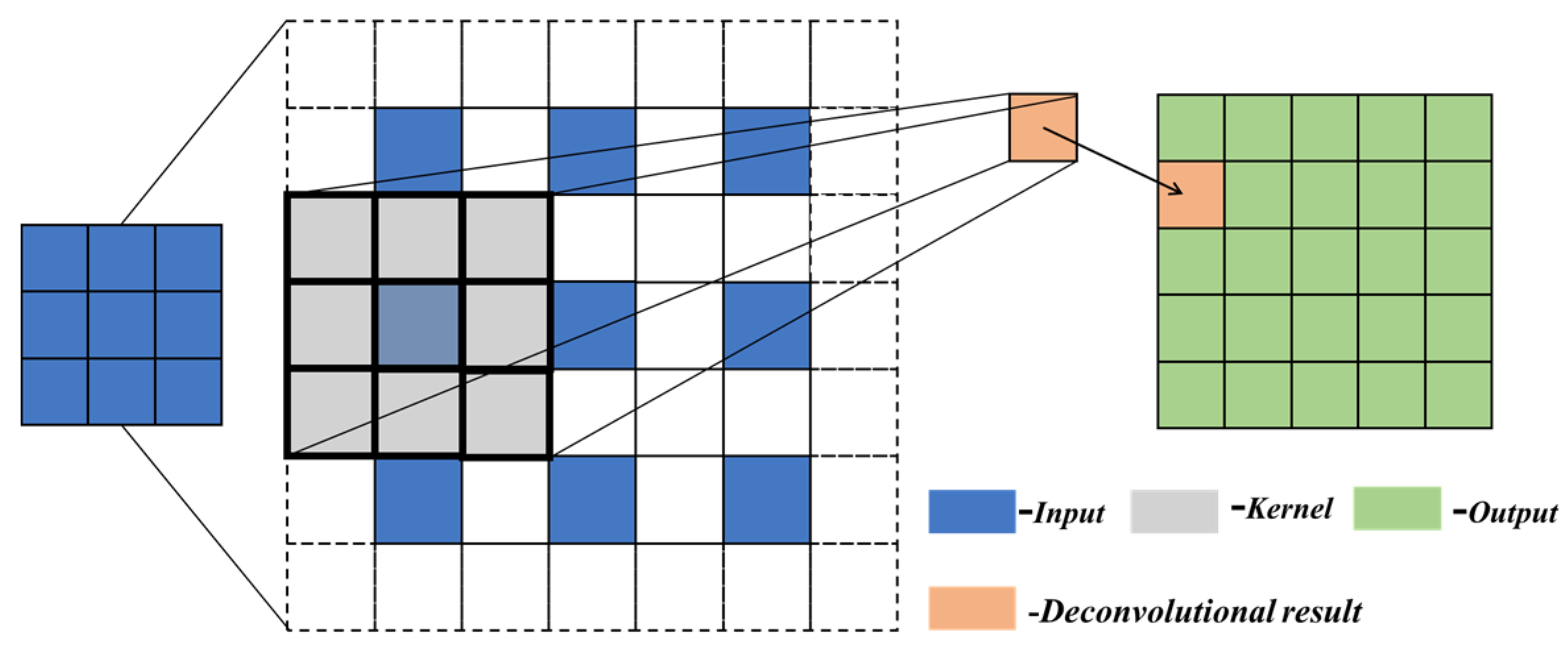
The deconvolutional operation is illustrated in Figure 2 with a simple example with padding size b = 1, stride size s = 2, and kernel size k = 3. For a more convenient description, the input, kernel, and output are marked in blue, gray, and green, respectively. The input of size 3 × 3 is interpolated with zero and the size of intermediate matrix up to (s × 3 + b) × (s × 3 + b), that is 7 × 7. The final output is the result of convolutional operation between the kernel and intermediate matrix with stride of 1. In this point, deconvolution can be seen as a kind of special convolution.
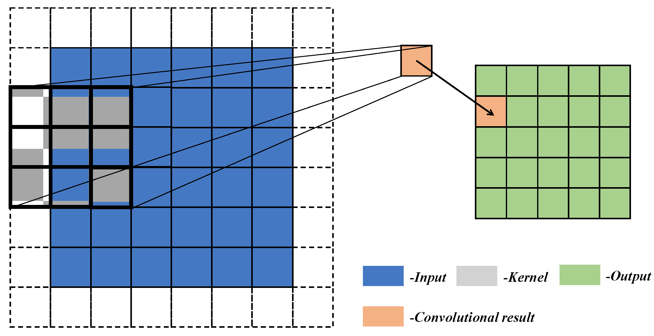
Convolutional neural networks became more and more popular in computer vision [33,34], nature language [35], and so on due to their powerful ability of feature extracting and learning. It is a natural idea to utilize convolutional neural networks to extract the low-dimensional performance from the high-dimensional physical fields. In mathematics, the convolution operation is a kind of multiplication of input and kernel at certain strides, as shown in Figure 3. Similar to Figure 2, the input, kernel, and output in this convolutional example are marked in blue, gray, and green, respectively. As shown in the sketch, the intermediate matrix can be obtained by input with padding around the original input matrix. Additionally, then the elements of output are the multiplication results of kernel and corresponding input elements moving at a specified stride.
With the complexity of application scenarios, the convolutional neural network goes deeper and deeper. However, some obstacles such as degradation of training accuracy and vanishing/exploding gradients arise with deeper layers. In order to avoid the above problems, some outstanding means, data normalization, intermediate normalization layers [36], and Residual Neural Network (ResNet) [37], were applied in our approach. In this study, input and output were normalized to (−1, 1) by maximum and minimum normalization, and batch normalization was applied after every deconvolution or convolution except for the output layer. The detailed architecture of our two-stage algorithm is listed in Table 1, in which Deconv2d means deconvolutional operation, Conv2d means convolutional operation, k is the size of kernel, s is the stride size, c is the channel size of output, in is the input size of linear layer, and out is the output size of linear layer. For more convenient description, the building block in ResNet is separated to the basic block (a pair of 3 × 3 filters) and shortcut (connection operation with identify) in this study. As shown in Table 1, the input of the field reconstruction model is firstly reshaped to a feature of large size by linear layer for subsequent deconvolutional operations. The size of output features become a specified 256 × 64 × 4 after the transformation of six deconvolutional layers and then the output features are interpolated to 256 × 64 × 4 and 256 × 64 × 4 for physical fields of stator and rotor blades. The similar interpolation operation can be found in performance prediction model. The physical fields with different sizes are adjusted to the specified size of 256 × 64 by an interpolation operation which makes the performance prediction model away from the affection of input size. After the subsequent convolutional operations from layer 1 to layer 6, the average pooling [38] and linear layers are adopted to obtain objective output from extracted features. In addition, the active function ReLU [39] is employed to enhance the nonlinear performance of the deep convolutional neural networks.
The Adaptive Moment Estimation (Adam) [40] optimizer was adopted in the optimization process. In essence, it is Root Mean Square Prop (RMSProp) [41] with a momentum factor. By combining the advantages of RMSProp and Adaptive Gradient (AdaGrad) [42], the Adam has lower calculation cost. In addition, it has good performance for high-dimensional space, large data sets, and most nonconvex optimization. Mathematically, the definitions of Adam are as follows:
t t 1
g t θ t ( θ t 1 )
m t β 1 · m t 1 + ( 1 β 1 ) · g t
v t β 2 · v t 1 + ( 1 β 2 ) · g t g t
m ^ t m t / ( 1 β 1 t )
v ^ t v t / ( 1 β 2 t )
α t α · 1 β 2 t ( 1 β 1 t )
θ t θ t 1 α t · m ^ t / ( v ^ t + ε )
where subscript t indicates the iteration step of the optimization process, is the loss function which can be s t a g e 1 or s t a g e 2 , θ is the learnable parameters of the neural network ( θ Θ 1   or   θ Θ 2 ), m is the first moment estimation, v is the second moment estimation, β1 and β2 are attenuation coefficients, α is the learning rate, and ε is a small number which prevents division by zero in the implementation. In this study, ε = 10−8, β1 = 0.9, and β2 = 0.999.
The optimization in stage 1 is performed such that the defined loss is minimized. Firstly, the field loss in this study is the mean square error (MSE) between the predicated field f ^ and the original field f , which can be written as:
f = E { x , f } ~ Γ ( l = 1 C | | f ^ i l f i l | | ) 1 N i = 0 N l = 1 C | | f ^ i l f i l | |
where N is the sample size and C is the number of fields in the train dataset. The subscript i represents sample index and the superscript l is the type of the field.
To circumvent a very blurred predication only by the field loss, the absolute error of gradient information between the predicated field and ground truth is reckon in loss function, also called gradient loss, that is defined as:
= E { x , f } ~ Γ ( l = 1 C | | · f ^ i l · f i l | | ) 1 N i = 1 N l = 1 C · f ^ i l · f i l
Then the total loss function to be minimized can be written as a combination of field loss and gradient loss, where λ is the loss weight. In this study, λ = 0.1.
stage 1 = F + λ
The optimization in stage 2 was performed to minimize MSE. For the batch of N samples, MSE of the parameterization case can be defined as:
stage 2 = 1 N m = 0 N ( y i t y i p ) 2
R square value (R2), mean absolute error (MAE), and root mean squared error (RMSE) are adopted to compare efficiency prediction results. R2, MAE, and RMSE are calculated using Equations (26)–(28), where Prei and Acti represent the predicted and actual efficiency and N is the number of observations in the testing dataset.
R 2 ( P r e , A c t ) = i = 1 N ( P r e i A c t i ) 2 / i = 1 N ( A c t i A c t ¯ ) 2
MAE ( P r e , A c t ) = 1 N i = 1 N | P r e i A c t i |
RMSE ( P r e , A c t ) = 1 N i = 1 N ( P r e i A c t i ) 2

3. Results and Discussion

3.1. CFD Off-Design Pre-Analysis

The design-optimization of a 60,000 rpm S-CO2 turbine were completed based on our previous research. First of all, the design-optimization approach using Gauss process regression was adopted [43]. Combined with the rapid 1-D thermal design method and the high-precision 3-D aerodynamic analysis method, the preliminary optimization design was obtained. Then, further 3-D aerodynamic optimization was carried out, mainly including inlet and outlet flow angle correction, flow matching of rotor and stator blades, blade profile optimization, etc. These optimization methods have achieved good results in previous research [24,44,45]. The detailed thermodynamic design parameters, geometric parameters, performance parameters, and blade profiles of the designed S-CO2 turbine are shown in Table 2.
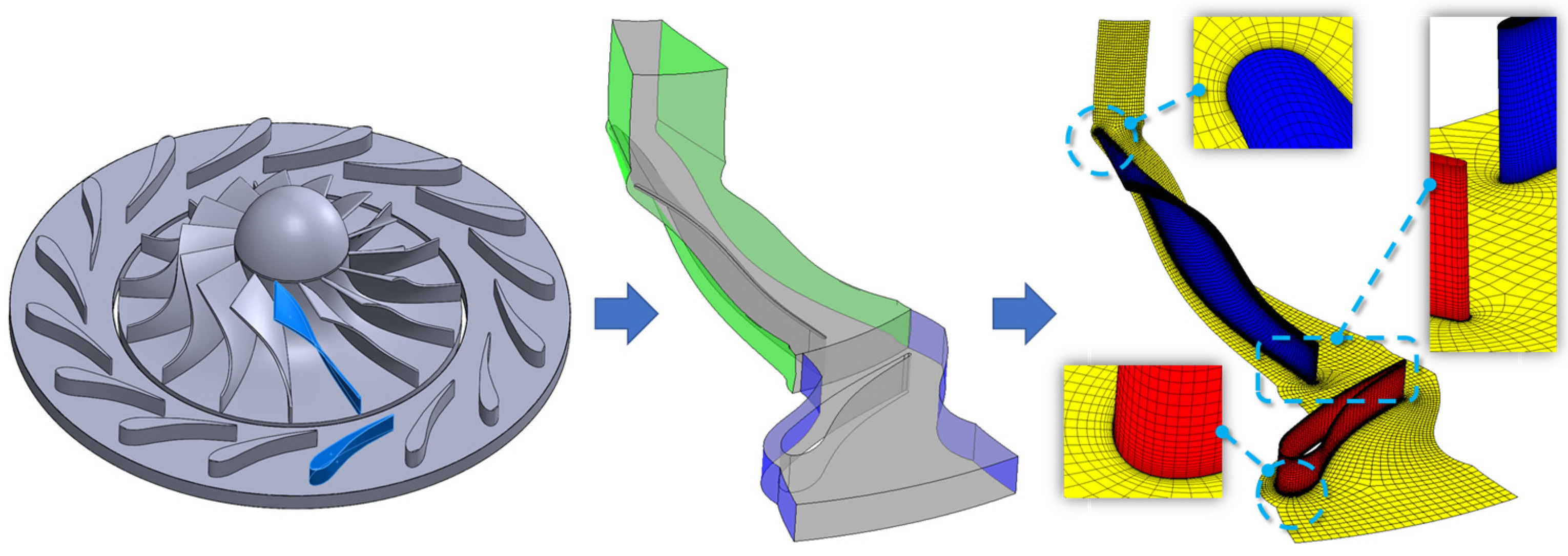
Figure 4 shows the 3-D model and numerical grid of the S-CO2 turbine. In this study, the single passage (one stator passage and one rotor passage) was used for calculation. In order to improve the mesh quality, the H type mesh was adopted in the inlet and outlet extension sections, while the O type mesh was adopted for blade meshing. The grids were densified in the tip clearance, around the blade and near the wall to obtain accurate flow parameters. The orthogonal angle of the mesh was greater than 15°, which meets the requirements of grid quality. The SST k ω turbulence model was adopted. The value of Y+ near the wall was about 1, which meets the calculation requirements of the turbulence model. The corresponding boundary conditions were given according to the thermodynamic design parameters. The grid independence was verified to balance the calculation accuracy and efficiency. The output power calculated at different grid scales was used as the evaluation basis. When the calculation error between adjacent grid scales is less than 1%, it is considered to meet the demand of calculation accuracy. The final number of selected grid nodes was 420,000. The numerical method was the same as previous research [24,43,44,45]. In previous research, the S-CO2 compressor with more complex flow was used for numerical verification. By comparing with the numerical and experimental results of other scholars, it can be shown that the numerical method is accurate [45]. For the off-design performance analysis of the turbine, the turbine’s inlet temperature, inlet pressure, inlet airflow angle, mass flow rate, and rotating speed were changed change within ±15% of the design value. The Latin Hypercube Sampling method was adopted to obtain a total of 1000 off-design conditions. The off-design performance data set of the designed turbine was obtained by CFD analysis of 1000 off-design conditions.
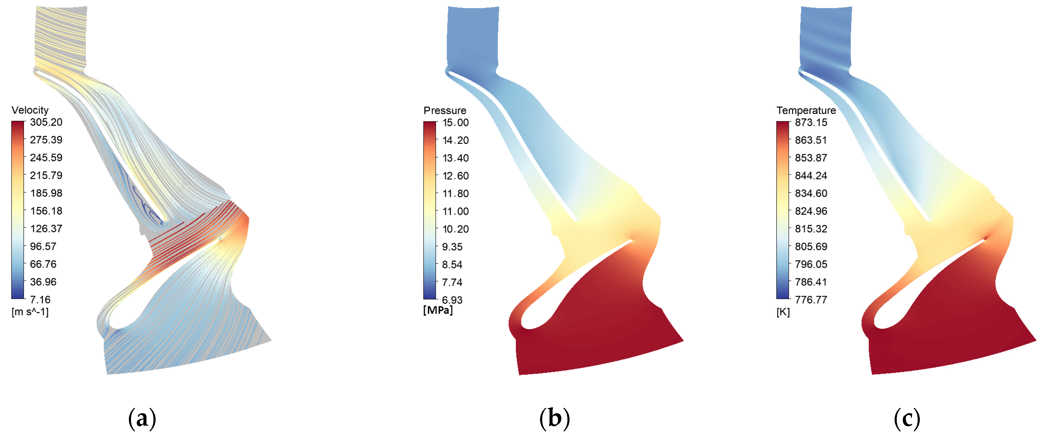
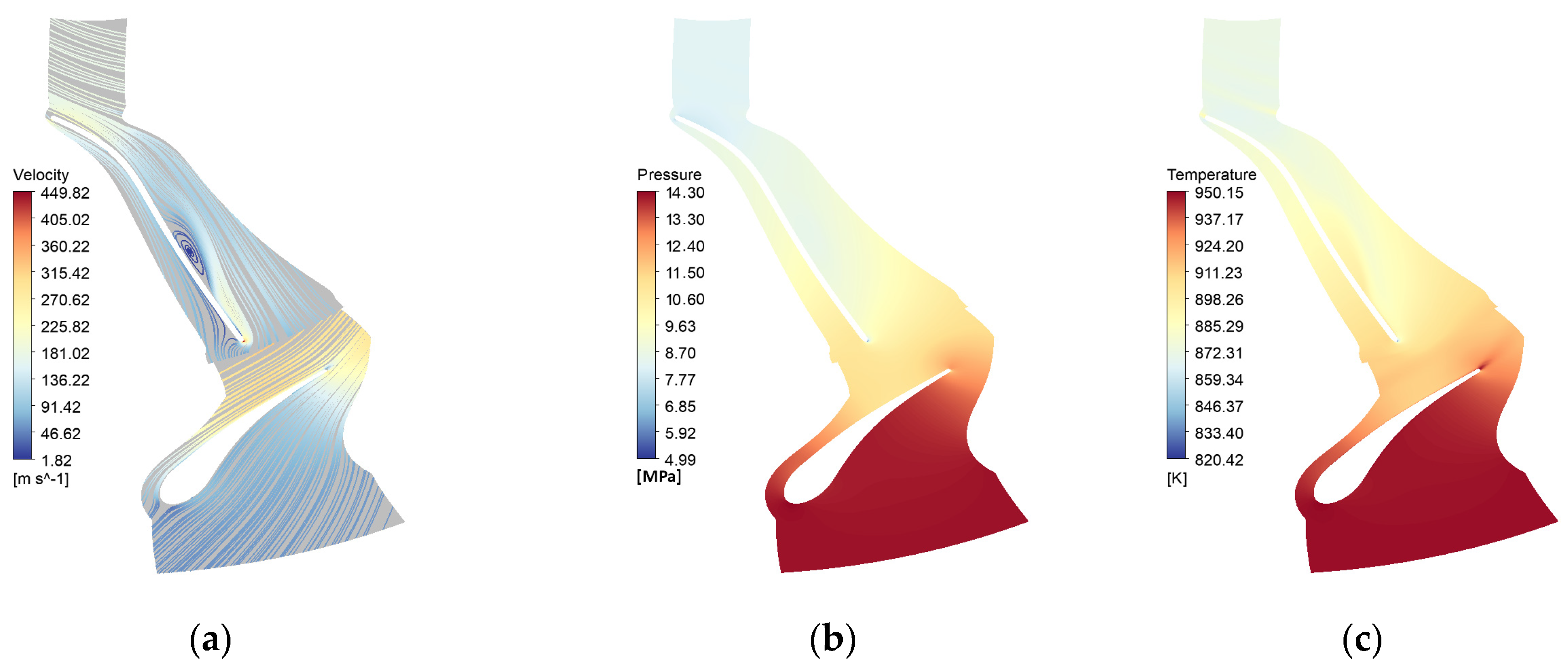
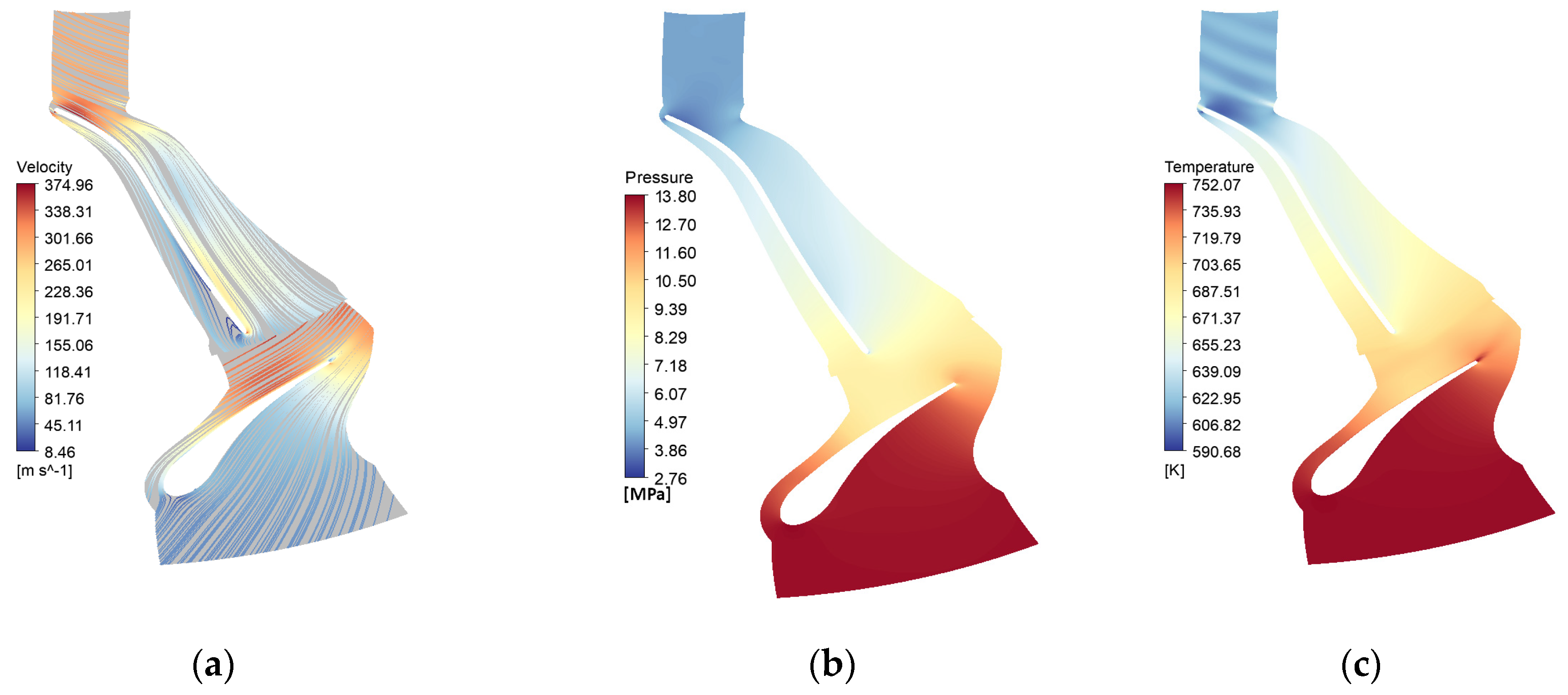
Table 2 shows that the output power of the designed S-CO2 turbine is 1019 kW and the total static efficiency is 89.44%. Figure 5 shows the limiting streamline, pressure distribution, and temperature distribution of the 50% blade height section of the turbine. At the inlet of impeller, the boundary layer thickens and even separates. This will cause great impact loss. Therefore, the turbine design in this paper adopts the negative impact angle design, which has less impact on energy loss than the positive impact angle. In addition, it can increase the power capacity of impeller [46,47]. It can be seen from the figure that except for a small range of flow separation phenomenon from the leading edge to 25% chord length on the pressure side of the rotor blade, there is no secondary flow in other flow passage areas. S-CO2 expands gradually from stator inlet to rotor outlet. The temperature and pressure decrease along the flow direction, and the value on the pressure side is larger than that on the suction side. There is no reverse pressure and temperature gradient. Therefore, the turbine design has good flow characteristics and aerodynamic performance. In order to explain the effect of prediction in detail, two off-design conditions, Case A ( x = [950.13 K, 14.27 MPa, 45.58°, 10.41 kg/s, 52,803.96 rpm]) and Case B ( x = [752.05 K, 13.80 MPa, 39.31°, 64,074.22 rpm]) are selected as examples in the design space. Figure 6 and Figure 7 show the limiting streamline, pressure distribution, and temperature distribution of Cases A and B, respectively. The results show that the operating conditions of Cases A and B are both away from the design point. There is a small range of flow separation or local acceleration in the turbine. The power and efficiency deviate greatly from the design condition. The power of Case A is 882.48 kW and the efficiency is 87.69%. The power and efficiency of Case B are 1608.73 kW and 83.07%, respectively.
The new 3-D CFD numerical analysis is often needed to predict the off-design performance of the turbine. In this method, the number of calculations is large, and the calculation speed is very slow. On the one hand, this will lead to a significant increase in the design cycle of the turbine. On the other hand, in the actual operation and control of the system, it is difficult to grasp the off-design performance of the turbine unit in real time. As a result, the system cannot be regulated in time. Therefore, it is urgent to develop an efficient and accurate prediction method of turbine performance under off-design conditions.

3.2. Physical Field Reconstruction

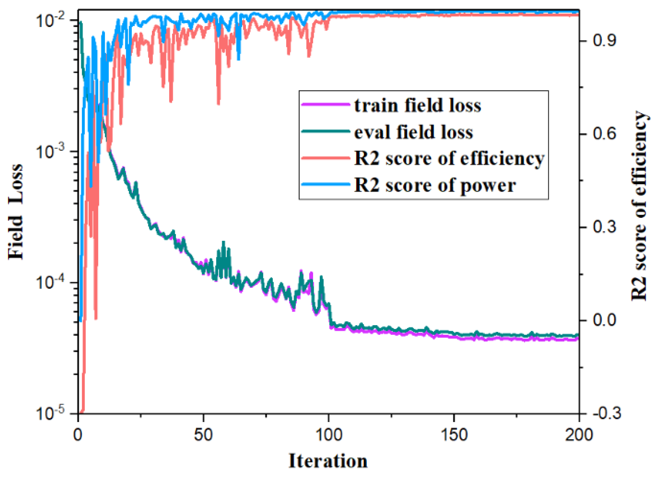
In this research, 70% and 30% of the off-design performance data set were selected as the training set and the verification set randomly for the neural network model training. The training process is shown in Figure 8. The cyan and purple lines indicate the field loss during the training process changes with the number of iterations. According to the figure, the field loss declines very quickly, and the loss of the training set and the verification set is similar in the late training period which can prove the model is well trained. The orange and blue lines indicate the R square value of the efficiency and power prediction, respectively, which can effectively represent the effect of the regression model. It can be seen from the figure that during the training process, the square R square value quickly rises from a large error area less than 0 to a small error close to 1 in the region. The final R-squared value is kept near 1, which means that all the real data in the validation set of the model we built predicts well.
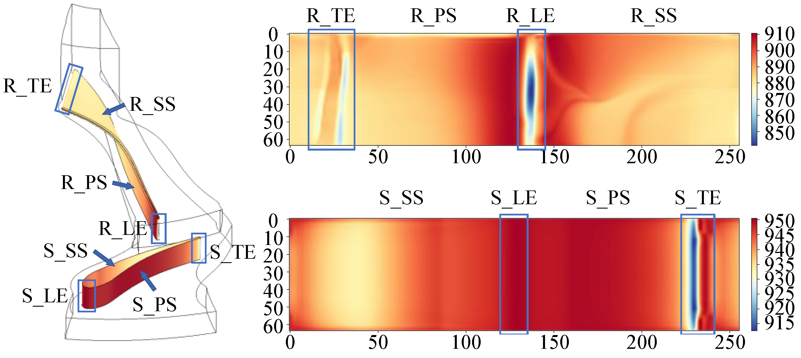
In this study, the surfaces of the stator blade and rotor blade were, respectively, expanded into the 260 × 65 rectangle as shown in Figure 9. The transverse direction is the chord direction, the longitudinal direction is the spanwise direction (0 for blade tip, 65 for blade root). Four key positions of leading edge (LE), trailing edge (TE), pressure surface (PS), and suction surface (SS) corresponding to rotor blade (R) and stator (S) blades were identified in the figure. For the rotor blade, area (12–40) × 65 corresponds to R_TE, area (130–145) × 65 corresponds R_LE, area (40–130) × 65 corresponds to R_PS, and the rest of the area corresponds to R_SS. For the stator blade, areas (120–135) × 65, (220–240) × 65, and (135–220) × 65 correspond to S_LE, S_TE, and S_PS respectively. The rest of the region corresponds to S_SS.
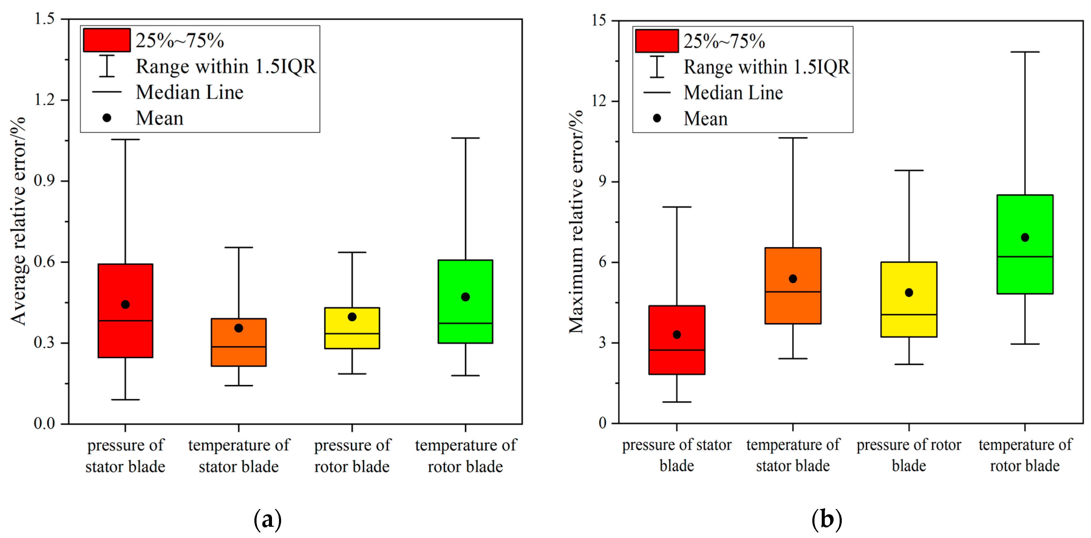
The data obtained after the reconstruction of all the calculation examples were summarized. Then, the average relative error and maximum relative error of the temperature and pressure at the stator blade and rotor blade were obtained with the box chart, as shown in Figure 10. The results show that the average relative error of the field is less than 1.5%, and the error of the stator blade temperature and the rotor blade pressure is relatively small. The maximum relative error is less than 15%, and the prediction error of the stator blade pressure is small. The above description shows that the reconstructed field is in good agreement with the field calculated by CFD, and the reconstruction method is effective.
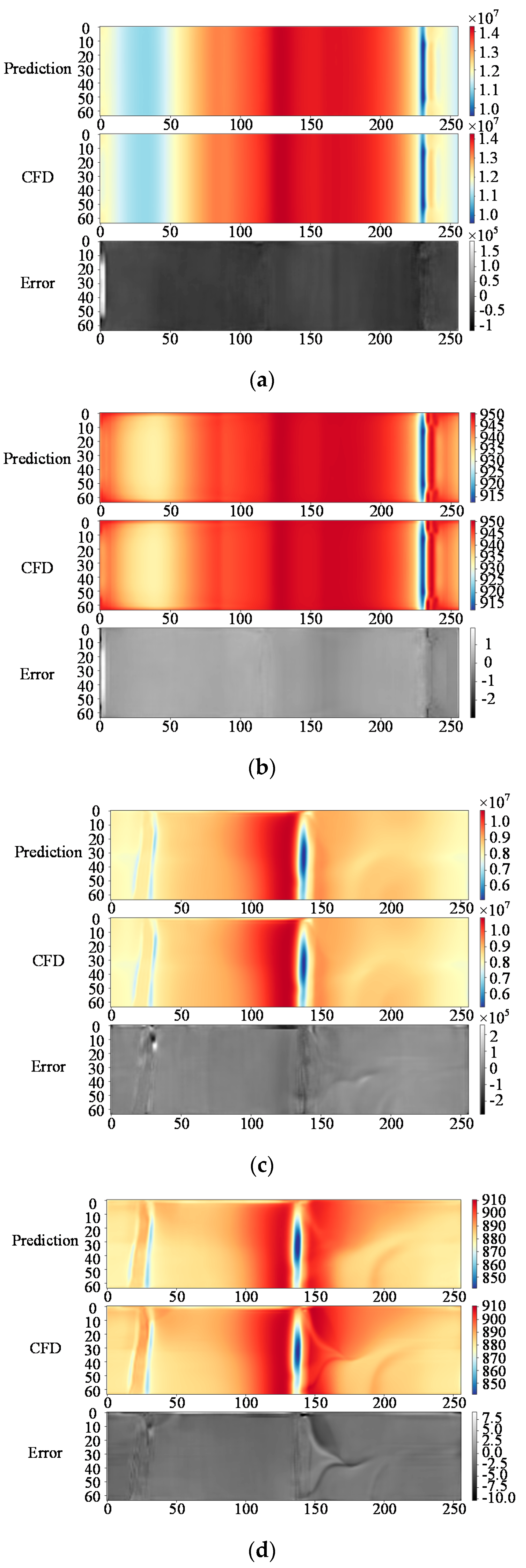
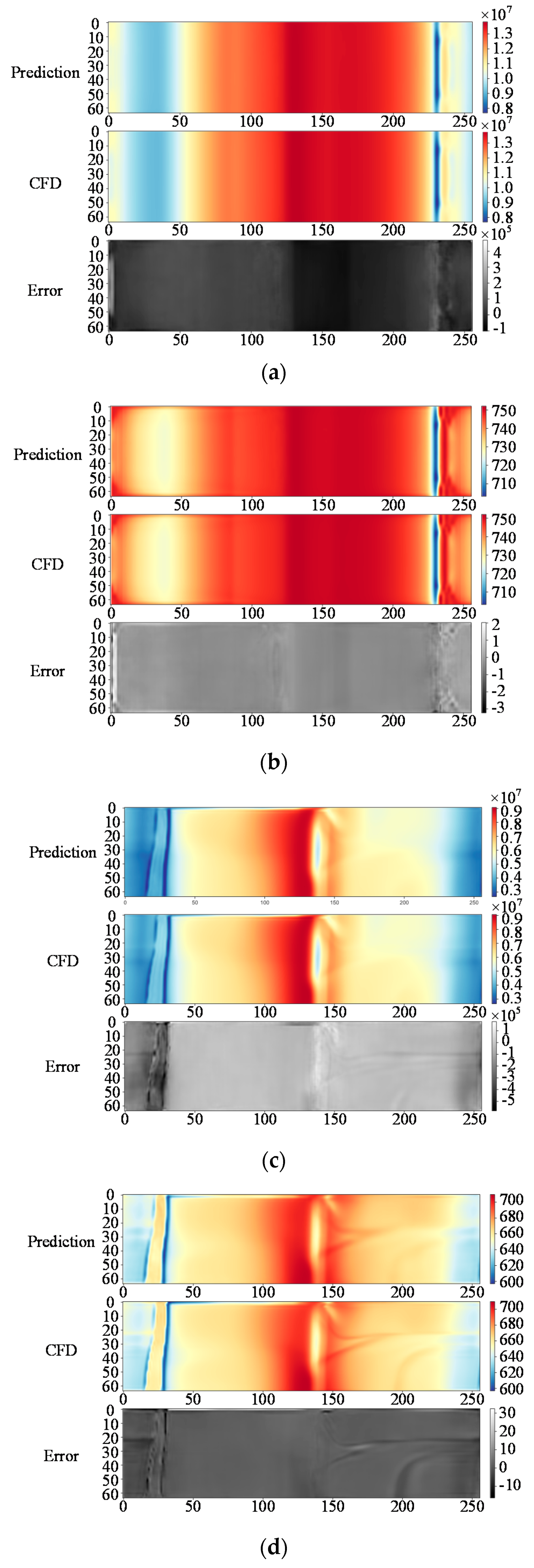
The prediction results, 3-D CFD results and error distributions of Cases A and B are shown in Figure 11 and Figure 12, respectively. It can be found that the cloud map distribution of the prediction results is basically the same as that of the CFD results, which is in good agreement. All kinds of key typical phenomena in turbine are captured and predicted, including:
  • Stagnation phenomenon of high temperature and high pressure in the S_LE.
  • The local acceleration of S_LE due to the large curvature change results in a small area of low pressure and low temperature.
  • The tip clearance of rotor blade is affected by the pressure difference between both rotor blade sides and the larger negative impact angle. This causes the working fluid in the tip clearance to accelerate from the pressure side to the suction side. Therefore, the pressure and temperature near the tip of the rotor blade will be relatively low.
  • The flow separation due to deviation from the design condition. It is worth noting that the flow in these regions is very complex, so the corresponding prediction error will increase accordingly. However, the error is still small, completely within the acceptable range.
The computation costs of different methods are compared in Table 3. The evaluation time of the CFD solver is the average time to obtain the numerical result with design input. Since ResNet based surrogate models could amortize computational overhead per instance by predicting multiple instances in parallel, we measured the average time cost for batch size 32 running on a Nvidia Geforce-1080. It can be found that GPU accelerated ResNet model only needs 0.04 s to obtain a prediction result. Compared with the conventional CFD method, our method can quickly predict the physical field on the blade surface and the aerodynamic performance of the turbine. It can greatly reduce the design cycle of the turbine. In addition, the off-design performance of the turbine unit can be mastered in real time in the actual operation of the system, so as to adjust and control the system in time and realize the rapid response of the system.

3.3. Performance Prediction

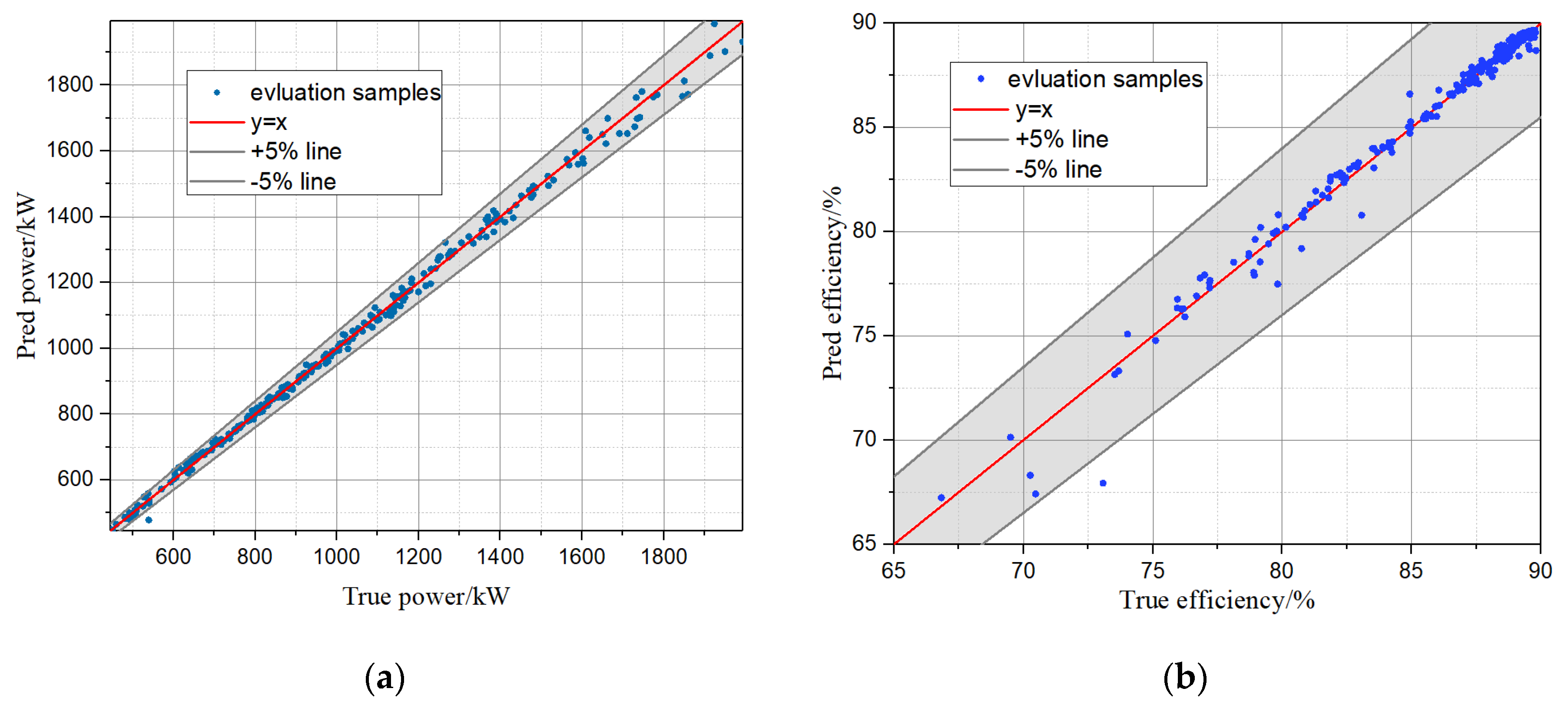
Based on the above physical field reconstruction results, the power and efficiency of the S-CO2 turbine were predicted under off-design conditions, as shown in Figure 13. The abscissa in the figure is the actual power and efficiency data calculated by numerical simulation. The ordinate is the power and efficiency data predicted by the model. The blue scattered points are the predicted sample points and the red line indicates that the prediction is completely correct at the ideal situation. The gray area indicates the distribution interval of the prediction error within 5%. The results show that basically all the prediction results of this model are within the distribution interval of 5%. The scattered points with poor prediction results are mostly in the low efficiency area.
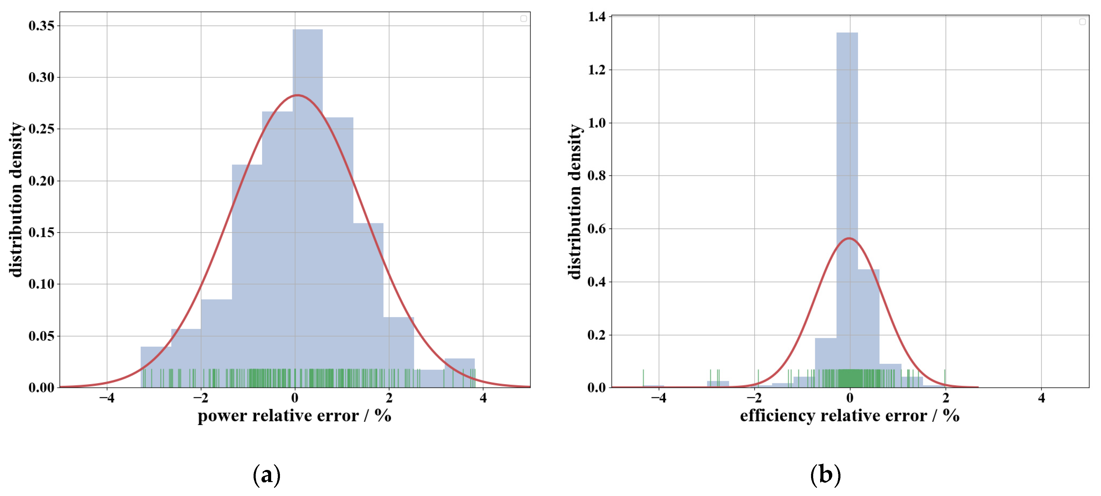
The detailed distribution density of power and efficiency in the range of ±5% relative error is shown in Figure 14. The relative error of power and efficiency are basically between −4% and 4%. The prediction of efficiency has a better effect, and the relative errors are concentrated in the ±1% range. It can be proved that the model in this research has high prediction accuracy.
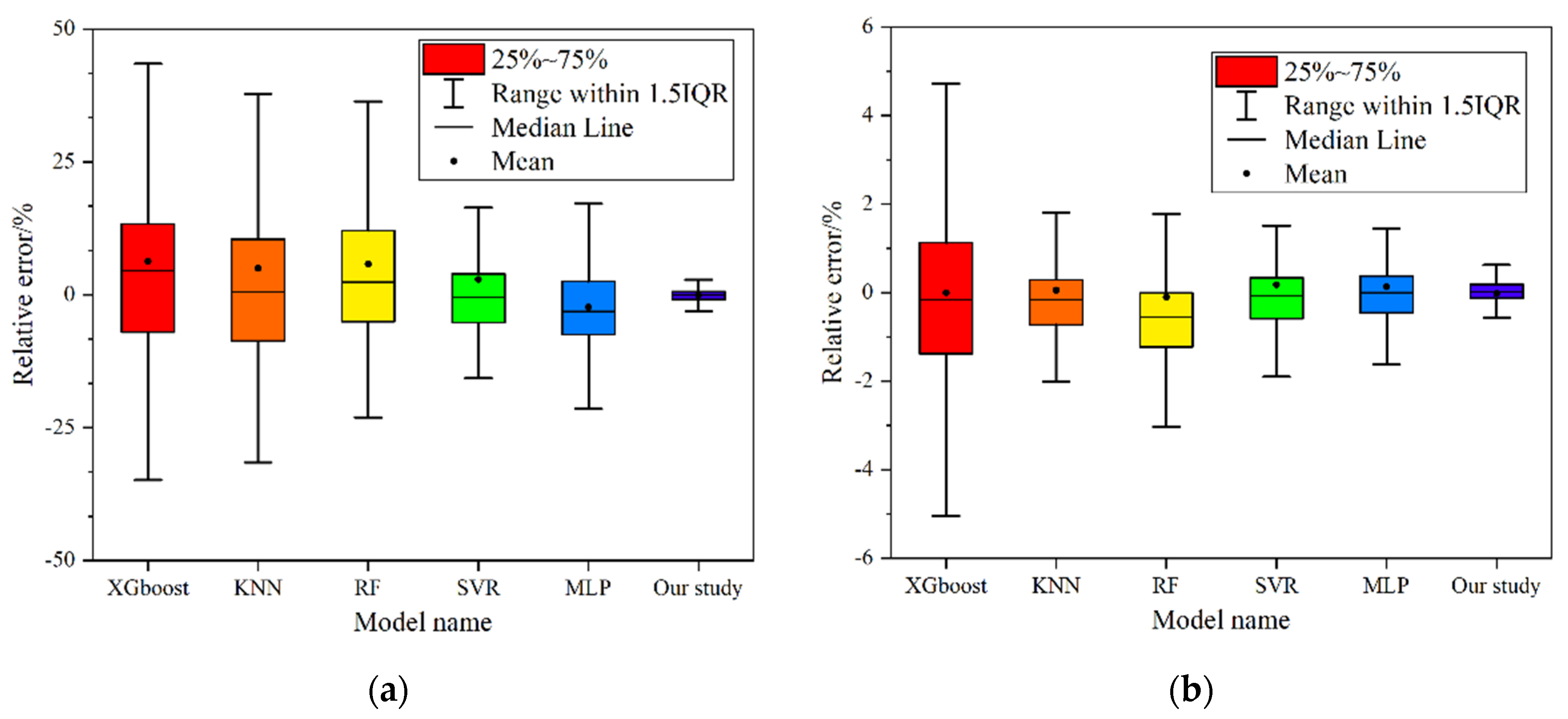
In this study, five classic data prediction methods of XGboost, KNN, RF, SVR, and MLP were compared with this model, as shown in Table 4 and Figure 15. The training and verification set of the above models are consistent. The evaluation index is the R2, MAE, and RMSE of the power and efficiency prediction result. The comparison of square values shows that the prediction efficiency of our model is the best.

4. Conclusions

In this research, we presented a two-stage deep convolutional neural network to predict the off-design performance of a S-CO2 turbine based on field reconstruction. The concrete results are listed as following:
  • The design and optimization of a 60,000 rpm S-CO2 turbine were completed based on our previous research. The output power of the designed turbine is 1019 kW and the total static efficiency is 89.44%.
  • At stage 1, the field reconstruction was conducted on 1000 off-design cases with varying design variables. The physical fields were plausibly predicted and all key typical phenomena in turbine were captured. The average relative error of the field is less than 1.5%, while the maximum relative error is less than 15%.
  • Based on the reconstructed physical field, the off-design performance of the S-CO2 turbine was predicted accurately at stage 2. The relative error of predicted power and efficiency are between −5% and +5%. Moreover, the relative error of efficiency is concentrated in the ±1% range.
  • Compared with other five classic data prediction methods, XGboost, KNN, RF, SVR, and MLP, the off-design power and efficiency prediction in this method clearly outperforms classical methods and comparable to a state-of-the-art model.
  • In addition, once the deep model is well-trained, the calculation with GPU-accelerated can quickly predict the physical fields on the blade surface and turbine performance.
Compared to the conventional off-design analysis methods, our method can provide more mechanism explanations for designers due to accurate prediction of physical fields. Our method relies on less human intervention and has the advantages of being effective, universal, flexible, and easy to implement, showing a good promise for real-time control and design optimization of turbines.

Author Contributions

Conceptualization, D.S. and Y.X.; investigation, D.S. and L.S.; methodology, D.S. and L.S.; resources, Y.X.; software, D.S. and Y.X.; supervision, Y.X.; validation Y.X.; writing—original draft preparation, D.S. and L.S.; writing—review and editing, D.S. All authors have read and agreed to the published version of the manuscript.

Funding

This research received no external funding.

Conflicts of Interest

The authors declare no conflict of interest.

References

  1. Gil, L.; Lacarra, S.O.; Embid, J.M.; Gallardo, M.A.; Blanco, S.T.; Artal, M.; Velasco, I. Experimental setup to measure critical properties of pure and binary mixtures and their densities at different pressures and temperatures: Determination of the precision and uncertainty in the results. J. Supercrit. Fluid 2008, 44, 123–138. [Google Scholar] [CrossRef]
  2. Crespi, F.; Gavagnin, G.; Sanchez, D.; Martinez, G.S. Supercritical carbon dioxide cycles for power generation: A review. Appl. Energy 2017, 195, 152–183. [Google Scholar] [CrossRef]
  3. Xie, Y.H.; Wang, Y.Q.; Zhang, D.; Shi, D.B. Review on Research of Supercritical Carbon Dioxide Brayton Cycle and Turbomachinery. Proc. Chin. Soc. Electr. Eng. 2018, 38, 7276–7286. [Google Scholar]
  4. Li, M.J.; Zhu, H.H.; Guo, J.Q.; Wang, K.; Tao, W.-Q. The development technology and applications of supercritical CO2, power cycle in nuclear energy, solar energy and other energy industries. Appl. Therm. Eng. 2017, 126, 255–275. [Google Scholar] [CrossRef]
  5. Manente, G.; Fortun, F.M. Supercritical CO2 power cycles for waste heat recovery: A systematic comparison between traditional and novel layouts with dual expansion. Energy Convers. Manag. 2019, 197, 111777. [Google Scholar] [CrossRef]
  6. Sun, L.; Wang, Y.; Wang, D.; Xie, Y. Parametrized Analysis and Multi-Objective Optimization of Supercritical CO2(S-CO2) Power Cycles Coupled with Parabolic Trough Collectors. Appl. Sci. 2020, 10, 3123. [Google Scholar] [CrossRef]
  7. Kim, D.Y.; Kim, Y.T. Preliminary design and performance analysis of a radial inflow turbine for ocean thermal energy conversion. Renew. Energy 2017, 106, 255–263. [Google Scholar] [CrossRef]
  8. Wright, S.; Radel, R.; Vernon, M.; Pickard, P. Operation and Analysis of a Supercritical CO2 Brayton Cycle; Sandia National Laboratories: Livermore, CA, USA, 2010.
  9. Cho, J.; Choi, M.; Baik, Y.J.; Lee, G.; Ra, H.-S.; Kim, B.; Kim, M. Development of the turbomachinery for the supercritical carbon dioxide power cycle. Int. J. Energy Res. 2016, 40, 587–599. [Google Scholar] [CrossRef]
  10. Zhou, A.; Song, J.; Li, X.; Ren, X.; Gu, C. Aerodynamic design and numerical analysis of a radial inflow turbine for the supercritical carbon dioxide Brayton cycle. Appl. Therm. Eng. 2018, 132, 245–255. [Google Scholar] [CrossRef]
  11. Han, W.; Zhang, Y.; Li, H.; Yao, M.; Wang, Y.; Feng, Z.; Zhou, N.; Dan, G. Aerodynamic design of the high pressure and low pressure axial turbines for the improved coal-fired recompression SCO2 reheated Brayton cycle. Energy 2019, 179, 442–453. [Google Scholar] [CrossRef]
  12. Luo, D.; Liu, Y.; Sun, X.; Huang, D. The design and analysis of supercritical carbon dioxide centrifugal turbine. Appl. Therm. Eng. 2017, 127, 527–535. [Google Scholar] [CrossRef]
  13. Yu, Y.; Chen, L.; Sun, F.; Wu, C. Neural-network based analysis and prediction of a compressor’s characteristic performance map. Appl. Energy 2007, 84, 48–55. [Google Scholar] [CrossRef]
  14. Rossi, M.; Renzi, M. A general methodology for performance prediction of Pumps-as-Turbines using Artificial Neural Networks. Renew. Energy 2018, 128, 265–274. [Google Scholar] [CrossRef]
  15. Palagi, L.; Sciubba, E.; Tocci, L. A neural network approach to the combined multi-objective optimization of the thermodynamic cycle and the radial inflow turbine for Organic Rankine cycle applications. Appl. Energy 2019, 237, 210–226. [Google Scholar] [CrossRef]
  16. Sarafraz, M.M.; Safaei, M.R.; Goodarzi, M.; Arjomandi, M. Experimental investigation and performance optimisation of a catalytic reforming micro-reactor using response surface methodology. Energy Convers. Manag. 2019, 199, 111983. [Google Scholar] [CrossRef]
  17. Sarafraz, M.M.; Tlili, I.; Tian, Z.; Bakouri, M.; Safaei, M.R. Smart optimization of a thermosyphon heat pipe for an evacuated tube solar collector using response surface methodology (RSM). Physica A 2019, 534, 122146. [Google Scholar] [CrossRef]
  18. Sarafraz, M.M.; Safaei, M.R.; Jafarian, M.; Goodarzi, M.; Arjomandi, M. High Quality Syngas Production with Supercritical Biomass Gasification Integrated with a Water–Gas Shift Reactor. Energies 2019, 12, 2591. [Google Scholar] [CrossRef] [Green Version]
  19. Guo, X.; Li, W.; Iorio, F. Convolutional Neural Networks for Steady Flow Approximation. In Proceedings of the 22nd ACM SIGKDD International Conference on Knowledge Discovery and Data Mining (KDD), San Francisco, CA, USA, 13–17 August 2016. [Google Scholar]
  20. Jin, X.; Cheng, P.; Chen, W.L.; Li, H. Prediction model of velocity field around circular cylinder over various Reynolds numbers by fusion convolutional neural networks based on pressure on the cylinder. Phys. Fluids 2018, 30, 047105. [Google Scholar] [CrossRef]
  21. Ti, Z.L.; Deng, X.W.; Yang, H.X. Wake modeling of wind turbines using machine learning. Appl. Energy 2020, 257, 114025. [Google Scholar] [CrossRef]
  22. Paszke, A.; Gross, S.; Chintala, S.; Chanan, G.; Yang, E.; DeVito, Z.; Lin, Z.; Desmaison, A.; Antiga, L.; Lerer, A. Automatic differentiation in PyTorch. In Proceedings of the NIPS Autodiff Workshop, Long Beach, CA, USA, 9 December 2017. [Google Scholar]
  23. Gao, K.K.; Xie, Y.H.; Zhang, D. Effects of stator blade camber and surface viscosity on unsteady flow in axial turbine. Appl. Therm. Eng. 2017, 118, 748–764. [Google Scholar] [CrossRef]
  24. Shi, D.B.; Zhang, L.; Xie, Y.H.; Zhang, D. Aerodynamic Design and Off-design Performance Analysis of a Multi-Stage S-CO2 Axial Turbine Based on Solar Power Generation System. Appl. Sci. 2019, 9, 714. [Google Scholar] [CrossRef] [Green Version]
  25. Menter, F.R. Two-equation eddy-viscosity turbulence models for engineering applications. AIAA J. 1994, 32, 1598–1605. [Google Scholar] [CrossRef] [Green Version]
  26. Winhart, B.; Sinkwitz, M.; Schramm, A.; Engelmann, D.; Di Mare, F.; Mailach, R. Experimental and Numerical Investigation of Secondary Flow Structures in an Annular Low Pressure Turbine Cascade Under Periodic Wake Impact—Part 2: Numerical Results. J. Turbomach. 2019, 141, 021009. [Google Scholar] [CrossRef] [Green Version]
  27. Mojaddam, M.; Hajilouy-Benisi, A.; Moussavi-Torshizi, S.A.; Movahhedy, M.R.; Durali, M. Experimental and numerical investigations of radial flow compressor component losses. J. Mech. Sci. Technol. 2014, 28, 2189–2196. [Google Scholar] [CrossRef]
  28. Zeiler, M.D.; Krishnan, D.; Taylor, G.W.; Fergus, R. Deconvolutional networks. In Proceedings of the IEEE Computer Vision and Pattern Recognition, San Francisco, CA, USA, 13–18 June 2010. [Google Scholar]
  29. Zeiler, M.D.; Taylor, G.W.; Fergus, R. Adaptive deconvolutional networks for mid and high level feature learning. In Proceedings of the IEEE Computer Vision and Pattern Recognition, Colorado Springs, CO, USA, 21–23 June 2011. [Google Scholar]
  30. Zeiler, M.D.; Fergus, R. Visualizing and understanding convolutional networks. In Proceedings of the Computer Vision—ECCV 2014: 13th European Conference, Zurich, Switzerland, 6–12 September 2014. [Google Scholar]
  31. Shelhamer, E.; Long, J.; Darrell, T. Fully Convolutional Networks for Semantic Segmentation. IEEE Trans Pattern Anal. Mach. Intell. 2017, 39, 640–651. [Google Scholar] [CrossRef]
  32. Radford, A.; Metz, L.; Chintala, S. Unsupervised representation learning with deep convolutional generative adversarial networks. In Proceedings of the 4th International Conference on Learning Representations (ICLR 2016), Caribe Hilton, San Juan, Puerto Rico, 2–4 May 2016. [Google Scholar]
  33. Krizhevsky, A.; Sutskever, I.; Hinton, G. ImageNet Classification with Deep Convolutional Neural Networks. In Proceedings of the Advances in Neural Information Processing Systems, Lake Tahoe, NV, USA, 3–6 December 2012. [Google Scholar]
  34. Simonyan, K.; Zisserman, A. Very Deep Convolutional Networks for Large-Scale Image Recognition. In Proceedings of the ICLR 2015: International Conference on Learning Representations 2015, San Diego, CA, USA, 7–9 May 2015. [Google Scholar]
  35. Li, K.P.; Wu, Z.Y.; Peng, K.C.; Ernst, J.; Fu, Y. Tell Me Where to Look: Guided Attention Inference Network. In Proceedings of the 31st IEEE/CVF Conference on Computer Vision and Pattern Recognition (CVPR), Salt Lake City, UT, USA, 18–23 June 2018. [Google Scholar]
  36. Ioffe, S.; Szegedy, C. Batch normalization: Accelerating deepnetwork training by reducing internal covariate shift. In Proceedings of the International Conference on Machine Learning, Lille, France, 6–11 July 2015. [Google Scholar]
  37. He, K.M.; Zhang, X.Y.; Ren, S.Q.; Sun, J. Deep Residual Learning for Image Recognition. In Proceedings of the IEEE Conference on Computer Vision and Pattern Recognition (CVPR), Las Vegas, NV, USA, 27–30 June 2016. [Google Scholar]
  38. Boureau, Y.L.; Bach, F.; Yann, L.C.; Ponce, J. Learning Mid-Level Features for Recognition. In Proceedings of the IEEE Conference on Computer Vision and Pattern Recognition (CVPR), San Francisco, CA, USA, 13–18 June 2010. [Google Scholar]
  39. Glorot, X.; Bordes, A.; Bengio, Y. Deep Sparse Rectifier Neural Networks. J. Mach. Learn. Res. 2011, 15, 315–323. [Google Scholar]
  40. Kingma, D.; Ba, J. Adam: A Method for Stochastic Optimization. In Proceedings of the ICLR 2015: International Conference on Learning Representations 2015, San Diego, CA, USA, 7–9 May 2015. [Google Scholar]
  41. Hinton, G.; Srivastava, N. Neural Networks for Machine Learning Overview of Mini-Batch Gradient Descent. Available online: https://www.cs.toronto.edu/~tijmen/csc321/slides/lecture_slides_lec6.pdf (accessed on 17 May 2019).
  42. Hadgu, A.T.; Nigam, A.; Diaz-Aviles, E. Large-scale learning with AdaGrad on Spark. In Proceedings of the IEEE International Conference on Big Data, Santa Clara, CA, USA, 29 October–1 November 2015. [Google Scholar]
  43. Shi, D.B.; Liu, T.Y.; Xie, Y.H.; Zhang, D. Design and Optimization of an S-CO2 Turbine Based on Gauss Process Regression. Chin. J. Power Eng. 2019, 39, 876–883. [Google Scholar]
  44. Shi, D.B.; Wang, Y.Q.; Xie, Y.H.; Zhang, D. The Influence of Flow Passage Geometry on the Supercritical Carbon Dioxide Centrifugal Compressor. Therm. Sci. 2017, 22, 253. [Google Scholar]
  45. Shi, D.B.; Xie, Y.H. Aerodynamic Optimization Design of a 150 kW High Performance Supercritical Carbon Dioxide Centrifugal Compressor without a High Speed Requirement. Appl. Sci. 2020, 10, 2093. [Google Scholar] [CrossRef] [Green Version]
  46. Fan, W.; Zhao, R.C.; Han, Z.H.; Wang, Z. Optimization of design parameters and thermodynamic design for radial flow turbine of organic working fluid. Acta Energy Sol. Sin. 2017, 38, 2309–2316. [Google Scholar]
  47. Wu, Z.Y.; Fang, X.J. Research on Variable Geometry Low Pressure Turbine Aerodynamic Performance. J. Propuls. Power 2018, 39, 269–276. [Google Scholar]
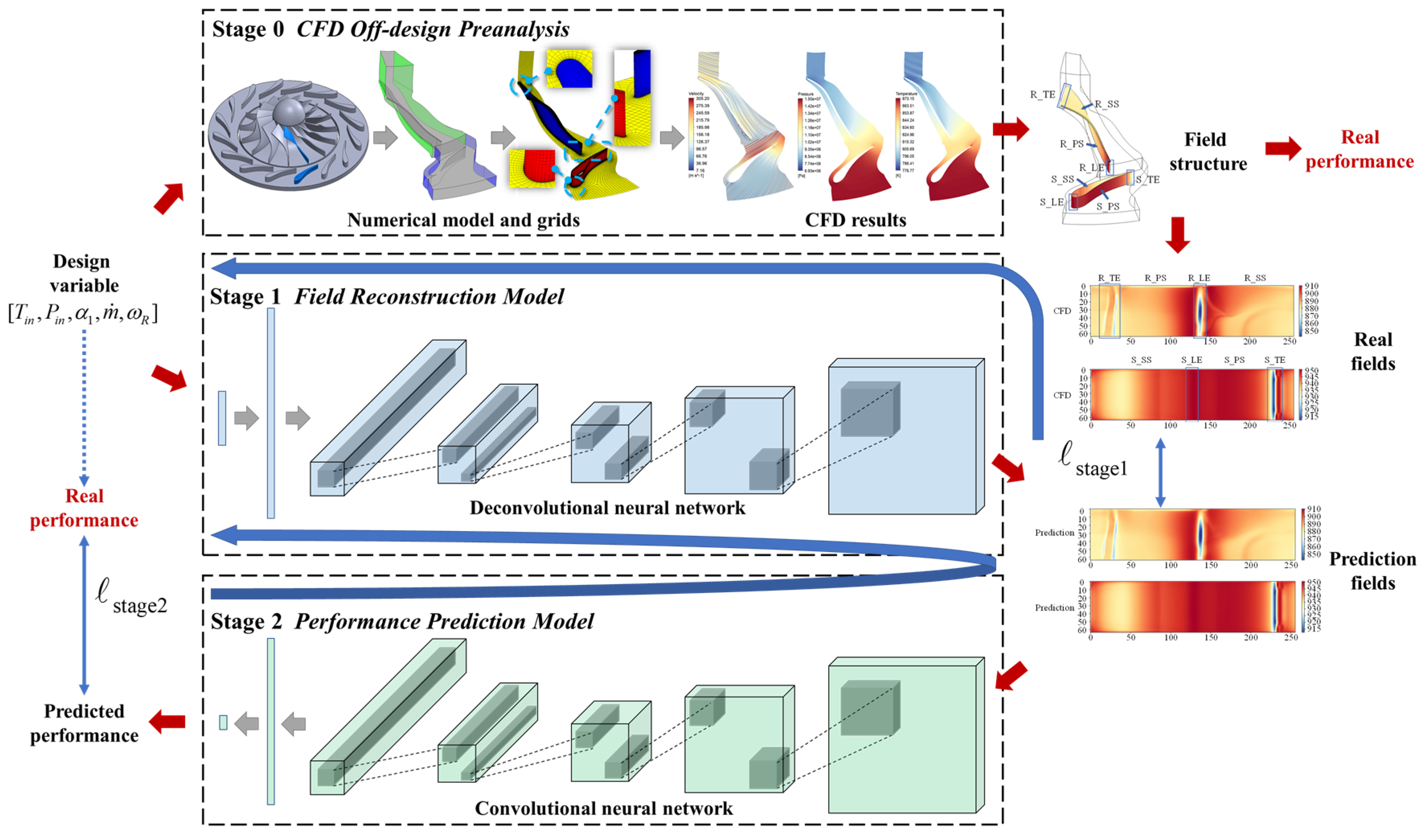
Figure 1. The overall architecture.
Applsci 10 04999 g001
Figure 2. A simple sketch of the deconvolutional layer.
Applsci 10 04999 g002
Figure 3. A simple sketch of the convolutional layer.
Applsci 10 04999 g003
Figure 4. 3-D numerical model and grids.
Applsci 10 04999 g004
Figure 5. Key parameter distributions of 50% blade height section under design conditions: (a) limiting streamline; (b) pressure distribution; (c) temperature distribution.
Applsci 10 04999 g005
Figure 6. Key parameter distributions of 50% blade height section of Case A: (a) limiting streamline; (b) pressure distribution; (c) temperature distribution.
Applsci 10 04999 g006
Figure 7. Key parameter distributions of 50% blade height section of Case B: (a) limiting streamline; (b) pressure distribution; (c) temperature distribution.
Applsci 10 04999 g007
Figure 8. The training process.
Applsci 10 04999 g008
Figure 9. Structure diagram of the field.
Applsci 10 04999 g009
Figure 10. The relative error: (a) the average relative error; (b) the maximum relative error.
Applsci 10 04999 g010
Figure 11. The parameter distribution of Case A: (a) the pressure of the stator blade; (b) the temperature of the stator blade; (c) the pressure of the rotor blade; (d) the temperature of the rotor blade.
Applsci 10 04999 g011
Figure 12. The parameter distribution of Case B: (a) the pressure of the stator blade; (b) the temperature of the stator blade; (c) the pressure of the rotor blade; (d) the temperature of the rotor blade.
Applsci 10 04999 g012
Figure 13. True-pre performance curve: (a) power; (b) efficiency.
Applsci 10 04999 g013
Figure 14. The distribution density of relative error: (a) power; (b) efficiency.
Applsci 10 04999 g014
Figure 15. Prediction results under different methods: (a) power; (b) efficiency.
Applsci 10 04999 g015
Table 1. Architecture of two-stage deep convolutional neural network.
LayersStage 1: Field Reconstruction ModelStage 2: Performance Prediction Model
Basic BlockShortcutBasic BlockShortcut
Input sizeBatch Size × 5 (number of design variables) Stator blade: Batch Size (64) × grid size (36 × 104)
Rotor blade: Batch Size (64) × grid size (51 × 232)
Input layerLinear (in = 5, out = 8192)Interpolation (Batch Size × 256 × 64 × 4)
Conv2d (k = 3, s = 1, c = 32)
Layer 1Deconv2d
(k = 3, s = 2, c = 512
Deconv2d
(k = 3, s = 1, c = 512)
Deconv2d
(k = 3, s = 2, c = 512)
Conv2d
(k = 3, s = 1, c = 64)
Conv2d
(k = 3, s = 1, c = 64)
Conv2d
(k = 3, s = 2, c = 64)
Layer 2Deconv2d
(k = 3, s = 2, c = 256)
Deconv2d
(k = 3, s = 1, c = 256)
Deconv2d
(k = 3, s = 2, c = 256)
Conv2d
(k = 3, s = 2, c = 128)
Conv2d
(k = 3, s = 1, c = 128)
Conv2d
(k = 3, s = 2, c = 128)
Layer 3Deconv2d
(k = 3, s = 2, c = 128)
Deconv2d
(k = 3, s = 1, c = 128)
Deconv2d
(k = 3, s = 2, c = 128)
Conv2d
(k = 3, s = 2, c = 256)
Conv2d
(k = 3, s = 1, c = 256)
Conv2d
(k = 3, s = 2, c = 256)
Deconv2d
(k = 3, s = 1, c = 128)
Deconv2d
(k = 3, s = 1, c = 128)
/Conv2d
(k = 3, s = 1, c = 256)
Conv2d
(k = 3, s = 1, c = 256)
/
Layer 4Deconv2d
(k = 3, s = 2, c = 64)
Deconv2d
(k = 3, s = 1, c = 64)
Deconv2d
(k = 3, s = 2, c = 64)
Conv2d
(k = 3, s = 2, c = 512)
Conv2d
(k = 3, s = 1, c = 512)
Conv2d
(k = 3, s = 2, c = 512)
Deconv2d
(k = 3, s = 1, c = 64)
Deconv2d
(k = 3, s = 1, c = 64)
/
Layer 5Deconv2d
(k = 3, s = 2, c = 32)
Deconv2d
(k = 3, s = 1, c = 32)
Deconv2d
(k = 3, s = 2, c = 32)
Conv2d
(k = 3, s = 2, c = 1024)
Conv2d
(k = 3, s = 1, c = 1024)
Conv2d
(k = 3, s = 2, c = 1024)
Layer 6Deconv2d
(k = 3, s = 1, c = 16)
Deconv2d
(k = 3, s = 1, c = 16)
Deconv2d
(k = 3, s = 1, c = 16)
AvgPool2d
(k = 3, s = 3)
Output layerConv2d (k = 3, s = 1, c = 4)
Interpolation (256 × 64)
Linear (in = 5120, out = 256)
Linear (in = 256, out = 2)
Output sizeStator blade: Batch Size (64) × grid size (36 × 104)
Rotor blade: Batch Size (64) × grid size (51 × 232)
Batch Size × 2 (number of performance)
Table 2. Key design parameters.
Parameter TypeParameterValueUnit
Thermodynamic parameterInlet temperature600°C
Inlet pressure15MPa
Outlet pressure8MPa
Design power1000kW
Rotating speed60,000rpm
Geometric parameterNumber of stator blades16pc.
Stator inner diameter119.7mm
Stator outer diameter153.2mm
Number of rotor blades15pc.
Impeller inlet blade height6mm
Impeller outer diameter99.7mm
Impeller outlet blade height15.9mm
Tip clearance0.2mm
Performance parameterMass flow rate11.38kg/s
Torque162.2N·m
Numerical power1019kW
Isentropic enthalpy drop1139kJ/kg
Total static efficiency89.44%
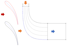
Blade profile Applsci 10 04999 i001
Stator (blade to blade) Rotor (Meridional plan)
Table 3. Comparison of computation costs with different methods.
MethodPhysical MemoryGraphics MemoryTrain TimeEvaluation Time
CFD solver730–1730 Mb//3.5 h
Our study—CPU1975–2975 Mb/24 h0.24 s
Our study—GPU2787–3787 Mb1785–2385 Mb4–5 h0.04 s
Table 4. Comparison with five classic data prediction methods.
ModelXGboostKNNRFSVRMLPOur Study
R20.67840.70200.74460.84470.90720.9851
MAE0.01840.01330.01480.00760.00660.0027
RMSE0.02970.02880.02670.02080.01610.0054