A Nonlinear Distortion Removal Based on Deep Neural Network for Underwater Acoustic OFDM Communication with the Mitigation of Peak to Average Power Ratio

Abstract

Machine learning and deep learning algorithms have proved to be a powerful tool for developing data-driven signal processing algorithms for challenging engineering problems. This paper studies the modern machine learning algorithm for modeling nonlinear devices like power amplifiers (PAs) for underwater acoustic (UWA) orthogonal frequency divisional multiplexing (OFDM) communication. The OFDM system has a high peak to average power ratio (PAPR) in the time domain because the subcarriers are added coherently via inverse fast Fourier transform (IFFT). This causes a higher bit error rate (BER) and degrades the performance of the PAs; hence, it reduces the power efficiency. For long-range underwater acoustic applications such as the long-term monitoring of the sea, the PA works in full consumption mode. Thus, it becomes a challenging task to minimize power consumption and unnecessary distortion. To mitigate this problem, a receiver-based nonlinearity distortion mitigation method is proposed, assuming that the transmitting side has enough computation power. We propose a novel approach to identify the nonlinear power model using a modern deep learning algorithm named frequentative decision feedback (FFB); PAPR performance is verified by the clipping method. The simulation results prove the better performance of the PA model with a BER with the shortest learning time.

1. Introduction

The demand for underwater wireless communication has increased tremendously with expected acceleration in the near future [1]. The multicarrier modulation techniques have become a hot research area in the last two decades. Orthogonal frequency divisional multiplexing (OFDM) is a multicarrier modulation technique that is popular in underwater acoustic (UWA) communication systems for transferring data [2]. However, an OFDM communication system has a major lack of high peak to average power ratio (PAPR). This results in lower power efficiency, creating problems while implementing UWA communication [3]. Besides this, there are several other limitations, such as characteristics of noise, multipath delay, and Doppler shift. These limitations bring great difficulties to the research and implementation of UWA communication [4,5]. Energy efficiency matters, particularly in UWA communication, for batteries deployed in underwater acoustic transceivers. Nowadays, a key driving factor is the growing energy cost of network operations, which can make up as much as 50% of the total operational cost [6]. By increasing the efficiency of a high-power amplifier (HPA), it can reduce energy costs. However, the HPA’s performance is directly linked to the input signal’s PAPR. Particularly in OFDM multicarrier transmissions, which are applied in many important wireless standards such as the Long-Term Evolution Advanced (LTE-A) Third Generation Partnership Project (3GPP) [7,8], the PAPR problem still prevents the adoption of OFDM in the uplink of mobile communication standards. It also affects the output power in the downlink coverage. It is necessary to find different methods to reduce the PAPR to a lesser value for a more powerful HPA, resulting in longer battery life and better efficiency [9]. For underwater acoustic sensing networks, there is the deployment of battery-powered modems in the water [4]. To maintain a sustainable network operation, it is necessary to reduce the PAPR of the OFDM signal [8]. For many applications, the problem of the PAPR can outweigh all the potential advantages of the OFDM communication system [10]. A variety of promising methods for the reduction of the PAPR has been proposed in the literature at the cost of BER, increment in transmission signal power, and computational complexity of the overall system. Therefore, in this paper, the PAPR of the underwater acoustic OFDM system is researched to design a nonlinear PA model with the help of a deep learning algorithm. Finally, we propose a receiver-based nonlinearity distortion mitigation method when the transmitting side has enough computation power. A nonlinear PA model is projected with the help of a modern deep learning algorithm; we call it FFB (frequentative decision feedback).

Related Work

Several pieces of literature have proposed a machine learning algorithm for the mitigation of the PAPR [4,11,12,13]. Before this study, we will discuss the nonlinearity reduction technique, which resulted in PAs. The first one is a PA with memoryless nonlinearity; the most common method used in this nonlinear PA model is the solid-state power amplifier (SSPA), soft limiter (SL), and traveling wave tube (TWT). For nonlinearity reduction, another PA model with memory nonlinearity is used, which is described in the literature [14,15,16,17,18].

The digital predistortion (DPD) algorithm is used in current telecommunication networks for the mitigation of PAPRs. A tremendous amount of research has been presented about the DPD. It deforms the signal before it goes to the PA in a way that the nonlinearity is reversed. It solves the problem of information loss due to nonlinear amplification in the PA. Hence, it is regarded as an adaptive and iterative process, which means the signal input and time will change its coefficients of DPD filters [19]. Thus, taking the inverse function of the PA input and output characteristics, an ideal predistorter can be formed. A large back-off is needed to resolve the nonlinearity problem; in other words, PBO (peak back-off) [20]. It is the difference in the power (dB) between the max desired output and the power of PA saturation. This makes a forceful operation by making the PA linear because the input passes through the nonlinear region of its characteristics and then the input power of the signal is reduced. When the value of the PBO is higher, it results in a higher BER and less efficiency.

Among all linearization methods, the DPD is the only choice selected by the industry. The DPD algorithm is briefly explained in [21,22]. In [7], the authors evaluated the performance of OFDM modulated symbols in a frequency-selective fading channel. The authors utilized a traveling wave tube (TWT) model of the PA in the article [23]. To reduce the nonlinearity, the authors presented novel research in the literature [24]—the signal constellation based on active constellation extension (ACE) built with a neural network termed time-frequency neural network (TFNN) is estimated. In this method, the time and frequency domain are considered simultaneously. The clipping technique is used to reduce the magnitude in the time domain. Furthermore, for the frequency domain, the constellation movement is restricted to only a few reasonable values. This model separates the real and complex parts of the symbols. The two neural networks are formed as $Mode{l}_{\mathit{Real}}^{TNN}$ and $Mode{l}_{\mathit{Imaginary}}^{TNN}$. The authors used the maximum likelihood method to detect the distorted symbols at the receiver. The autoencoder scheme for the reduction of the PAPR in the literature [25] uses the autoencoder of deep learning termed PRNet. The PRNet method performs well in both PAPR and BER at the cost of computational complexity. The deep neural network-based OFDM receiver has been proposed in the literature [26,27] for UWA communication. The authors used a single neural network to implement aggregate signal processing. This method was tested by using a ray-tracing toolbox with a sound speed profile (SSP) measured in a real sea experiment. In the research [28], the authors adopted adaptive modulation for reducing the filter concatenation effect for optical OFDM communication. The transmission performance was improved by up to 60%. Four types of optical filters, including fiber Bragg grating (FBG), wavelength-selective switch (WSS), thin film, and Chebyshev, were used to evaluate system’s performance. The power loading (PL), bit loading, and bit-and-power (BPL) loading algorithms were introduced in the literature [29] by over 1000 statistically constructed worst-case multimode fiber (MMF) links without incorporating inline optical amplification. The authors proposed compressed sensing (CS) in [30,31,32] for mitigation of clipping noise in UWA communication. This scheme exploited pilot tones and data tones instead of reserved tones which is different from traditional clipping methods. It provides more accurate UWA channel characteristics for estimating the clipping noise than traditional methods such as Least square (LS) and measuring mean squared error (MMSE).

The proposed algorithm is named FFB, which detects nonlinear distortion at the receiver side. Our method is based on research [14]. The method used in [33] is an extension approach of the literature [14]. The proposed PA model is called a memory device whose output depends upon the OFDM symbols. The channel estimation was performed using pilot symbols. In this process, only a few carriers were active. It makes sure that the value of the PAPR is low, and the PA mostly operates in a linear region. 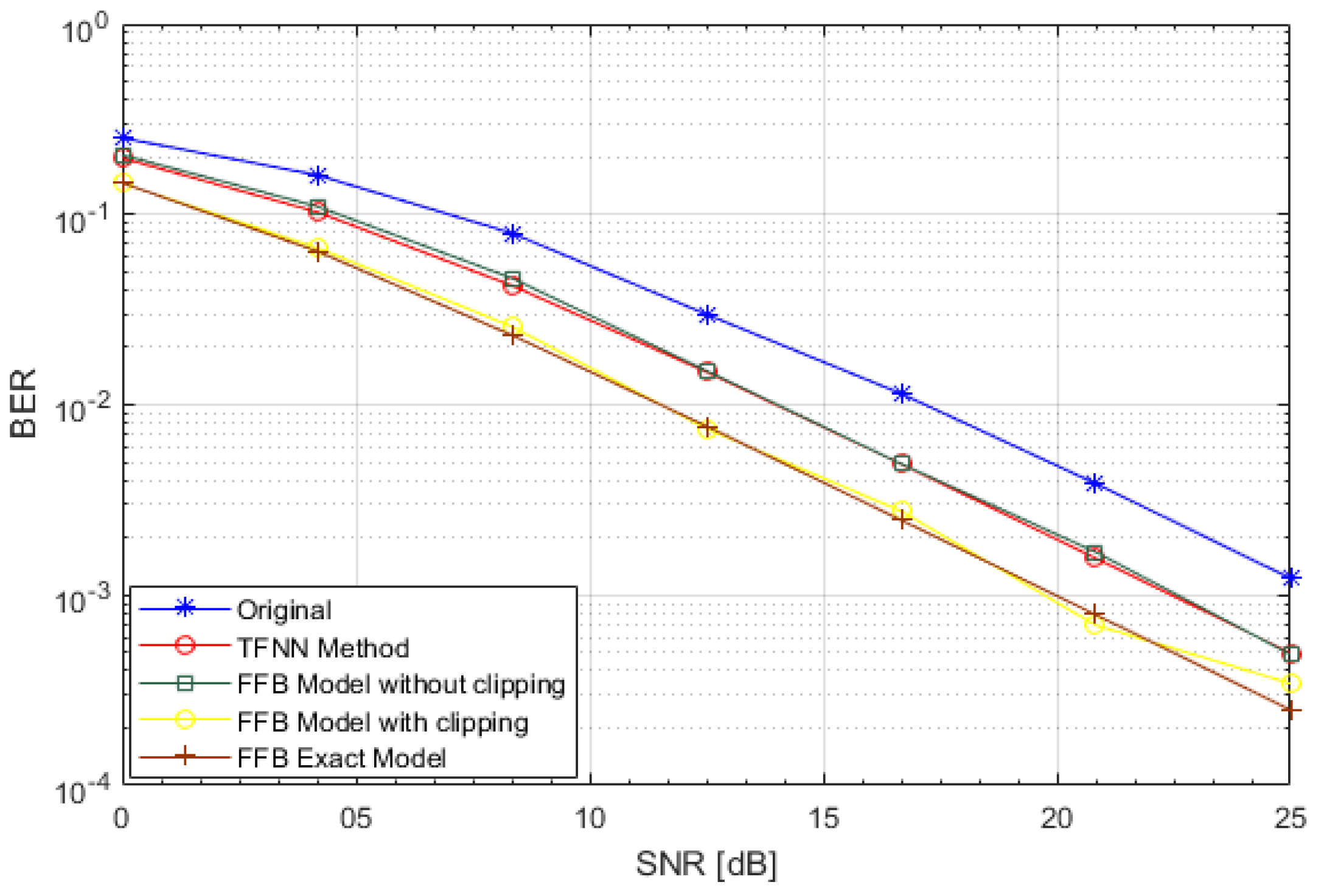In this paper, we have used the approach used in [14]; we named this method FFB. The FFB model is used to mitigate the nonlinearity of the PAPR. Firstly, the PAPR is reduced in an OFDM system with a clipping technique. Secondly, the unnecessary distortion caused by high PAPRs is reduced at the receiver side by using a modern neural network. This model is trained with a machine learning algorithm with a proper set of data. Collectively, the channel coefficient fits best to the maximum likelihood model, and the performance is improved in terms of the BER and higher efficiency.

2. System Model

In this section, we discuss the effect of the PAPR in OFDM modulated signals, and how it affects the communication system and the BER and degrades performance. The lower-case $x$ is used for time-domain values, and for frequency-domain values, we use $X$ upper-case values. Furthermore, the complex conjugate of $x$ is denoted by $x^{\ast }$. The vectors are represented as boldface or sequence x[n], e.g., $x[n]=[x_0,\dots .x_{N-1}]$. 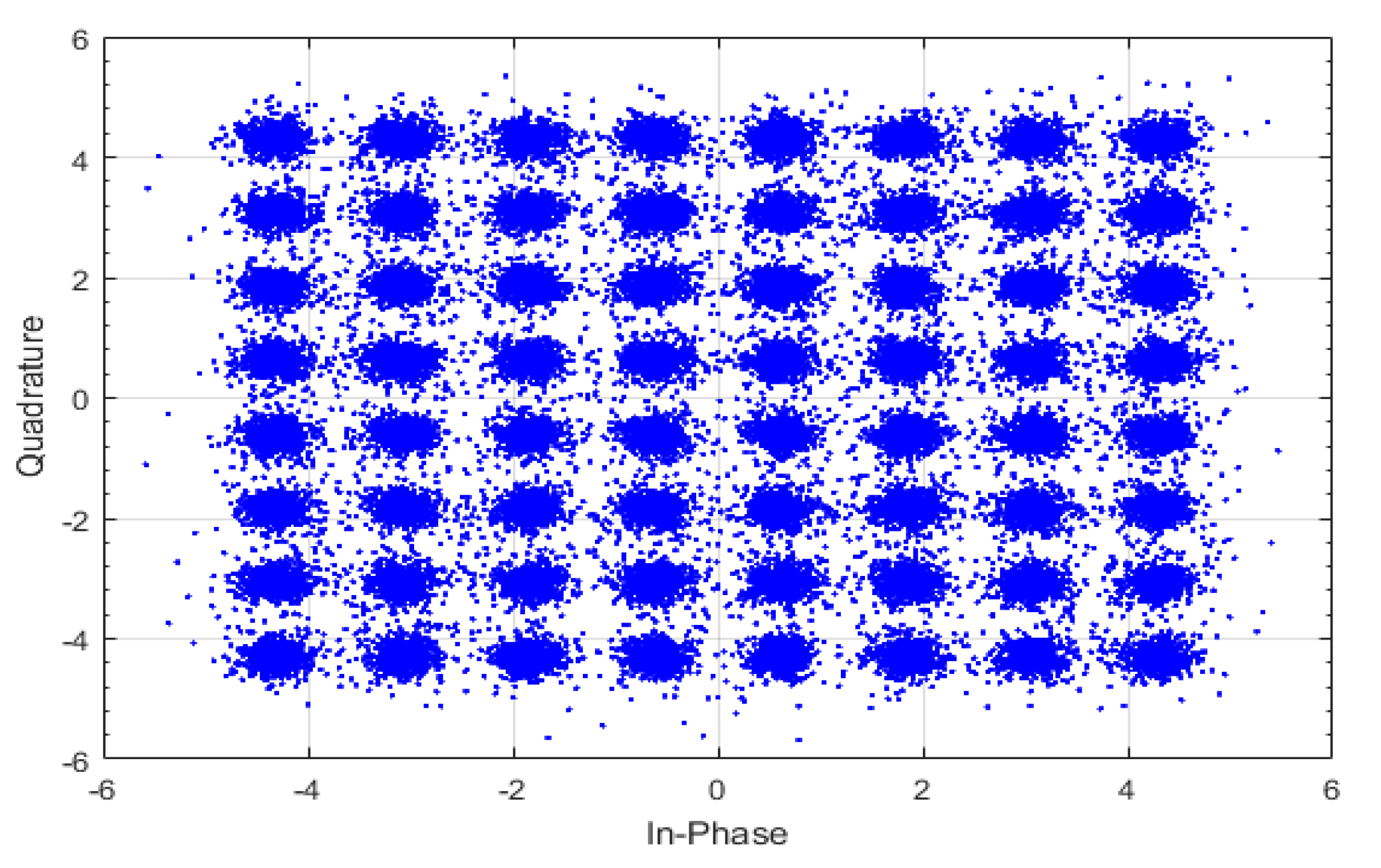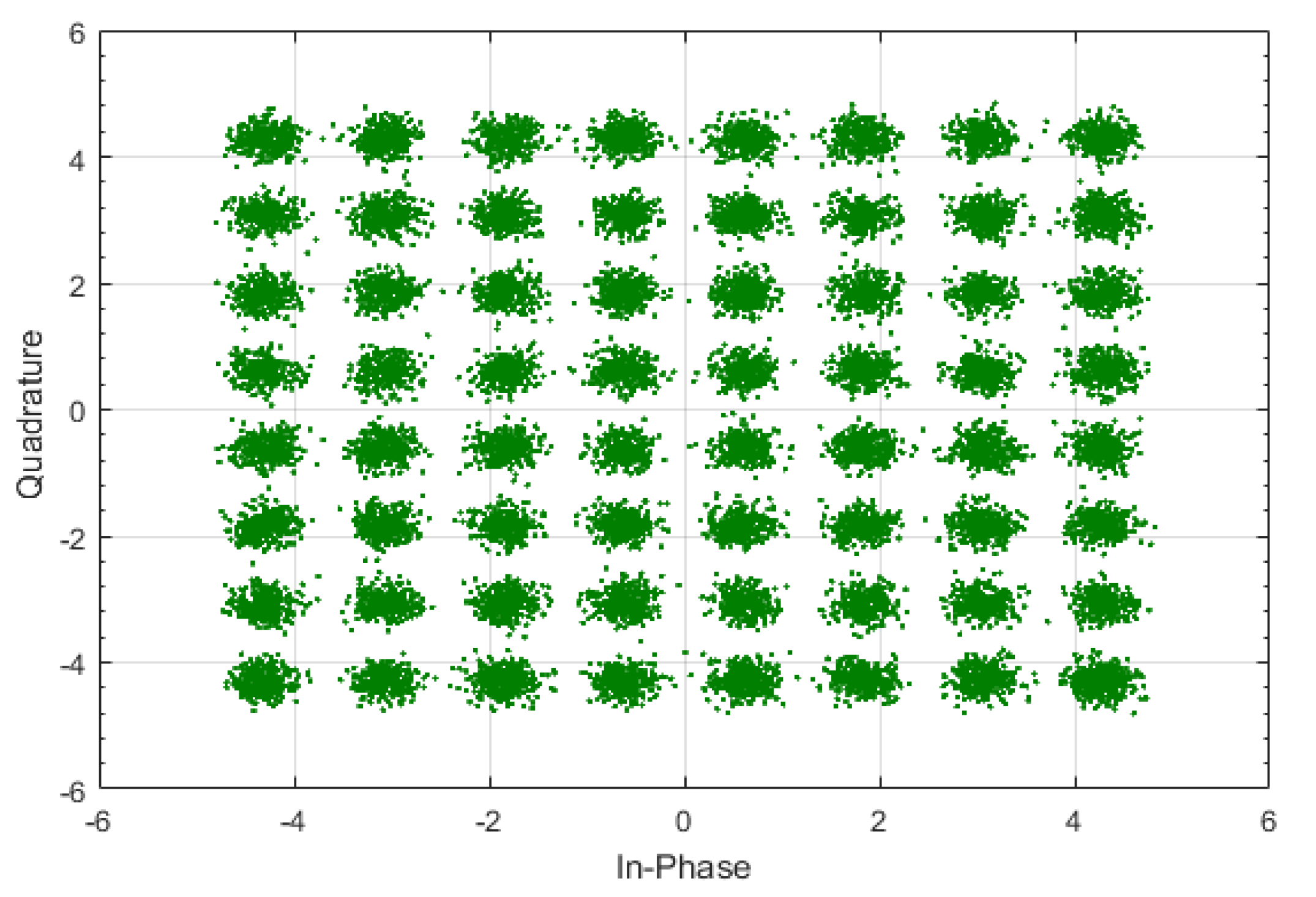The frequency is denoted as $k$, and index n stands for time. In order to better understand the PAPR, the OFDM-modulated symbols were analyzed more deeply. We consider the quadrature amplitude modulation (QAM) symbols $[X(0),\dots .,X(N-1)]$; these are modulated over subcarriers $0..n$. Each of the QAM has maximum amplitude as $a_n=\pm a$, separated by a bandwidth B of Hz or a duration of $T=\frac{1}{B}$ seconds. Each OFDM symbol comprises of N, equally spaced QAM symbols. It can be written mathematically as

$$x^p(t)=\frac{1}{\sqrt{N}}{\displaystyle \sum _{K=\frac{-N}{2}}^{\frac{-N}{2}-1}{X}_k^{p}e\frac{j2\pi kt}{T}}$$

(1)

The OFDM symbol index is denoted by p; $X_k^p$ represents the QAM value of $k^{th}$ subsymbol. To avoid the intersymbol interference (ISI) and make channel flat fading in each subcarrier, the CP cyclic prefix is added; the length of the CP is greater than the delay spread of the channel. Some part of the signal $x_n(t)$ is copied from the end, and we add it to the front of the transmit signal. Hence, the signal transmitted with a cyclic prefix can be represented by Equation (2).

$$x_{transmit}(t)=x(N-L+1)\dots \dots x(N-2)x(N-1)x(0)x(1)\dots \dots x(N-2)x(N-1)$$

(2)

where the last L symbols are added together in a series at the front of the OFDM symbol block. The IFFT is used to generate $x_{transmit}(t)$. Before the IFFT operation, the signal is converted from serial to parallel, then it is upsampled by a factor L. Upsampling can be regarded as one way of pulse shaping in an OFDM. After these two operations of upsampling and IFFT, the transmitted digital signal can be represented as

$$x^p[\frac{n}{L}]=\frac{1}{\sqrt{N}}{\displaystyle \sum _{k=\frac{-N}{2}}^{\frac{N}{2}-1}{X}_k^p{e}^{\frac{j2\pi kn}{NL}}}$$

(3)

$${\displaystyle \sum _{k=0}^{\frac{N}{2}-1}{X}_k^p{e}^{\frac{j2\pi kn}{NL}}}+{\displaystyle \sum _{k=NL-\frac{N}{2}}^{NL-1}{X}_{k-N(L-1)}^p{e}^{\frac{j2\pi kn}{NL}}}$$

(4)

$$=IFFT([X_0^p\dots \dots X_{\frac{N}{2}-1}\underset{\hspace{0.17em}N(L-1)}{0,\dots \dots ,0}{X}_{\frac{Np}{2}}\dots \dots X_{N-1}^p])$$

(5)

where $X_L^P$ is L times the oversampled QAM vector. Hence, the transmitted symbols are $[x^p(0),x^p(1),x^{(p)}(2)\dots \dots x^p(N-1)]$, which are the IFFT of the upsampled QAM symbols $[X_0^p\dots \dots X_{\frac{N}{2}-1}\underset{\hspace{0.17em}N(L-1)}{0,\dots \dots ,0}{X}_{\frac{N}{2}}p\dots \dots X_{N-1}^p]$.

2.1. PAPR

Let us calculate the average power of OFDM symbols and derive a mathematical relationship between the PAPR and OFDM number of subcarriers in this subsection. Firstly, the average of OFDM symbols is calculated. The PAPR can be defined as the ratio of max (transmitted signal)/average transmitted power. It can be written as

$$PAPR=\frac{\max \left|x_n\right|}{E[{\left|x_n\right|}^2]}$$

(6)

Here $E[{\left|x_n\right|}^2]$ is the average signal power.

The average signal power is evaluated further as = $E[x(n).x^{\ast }(n)]$

$$=\frac{1}{N^2}.E[{\displaystyle \sum _{i=\frac{-N}{2}}^{\frac{N}{2}-1}{a}_n.{\exp }^{\frac{j2\pi ki}{N}}}{\displaystyle \sum _{i=\frac{-N}{2}}^{\frac{N}{2}-1}{a}_n^{\ast }.{\exp }^{\frac{-j2\pi ki}{N}}}]$$

(7)

$$=\frac{1}{N^2}E[a_n.a_n^{\ast }{\displaystyle \sum _{i=\frac{-N}{2}}^{\frac{N}{2}-1}{\displaystyle \sum _{i=\frac{-N}{2}}^{\frac{N}{2}-1}{\exp }^{\frac{j2\pi ki}{N}}{\exp }^{\frac{-j2\pi ki}{N}}}}]$$

(8)

Since $E[{\left|{\exp }^{\frac{2\pi ki}{N}}\right|}^2]$ is a phase factor, if it is equal to 1, also $a_n.a_n^{\ast }=a^2$, then

$$\begin{array}{l}=\frac{1}{N^2}{\displaystyle \sum _{i=\frac{-N}{2}}^{\frac{N}{2}-1}{a}^2}\\ =\frac{1}{N^2}.a^2.N=\frac{a^2}{N}\end{array}$$

(9)

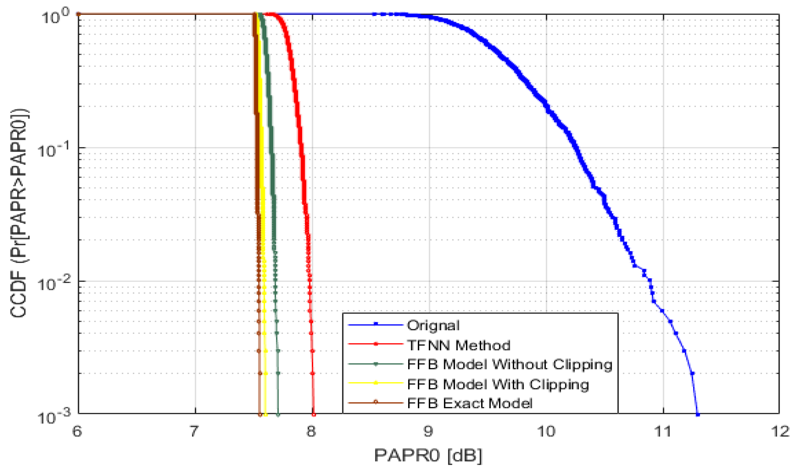
Thus, the average power of transmission is $\frac{a^2}{N}$. To analyze the peak power when QAM symbols have an amplitude of $\pm a$, we consider all the information symbols of QAM as $[X(0).X(1)\dots .X(N-1)]$, which has an amplitude of $+a$

$$\begin{array}{l}x(0)=\frac{1}{N}{\displaystyle \sum _{i=\frac{-N}{2}}^{\frac{N}{2}-1}X(i)}\\ =\frac{1}{N}.N.a=a\end{array}$$

(10)

Hence, we see that the peak power is $a^2$. The ratio of peak to average power (PAPR) $=\frac{a^2}{\frac{a^2}{N}}=N$. N is the number of subcarriers, which can be 32, 64, 128, 256, or more than 512. In conclusion, the PAPR in an OFDM system is high when the number of subcarriers increases by order because the symbols of data in the subcarriers are added up, which produces the high peak valued signals. The signal which passes through a PA or transmitting transducer can be split into two different components. The first one is a distorted part, and the second is with no distortion. By doing this, we have an opportunity to estimate the distorted part of the signal at the receiver side. If the model of the PA is known, then the distortion term can be estimated efficiently. Therefore, the machine learning algorithm can help us to assess the PA model at the receiving side. The performance and computational capabilities of this algorithm are very high, and it can estimate accurately. Hence, this allows us to design a signal processing algorithm that will estimate the distortion term and give us improved performance.

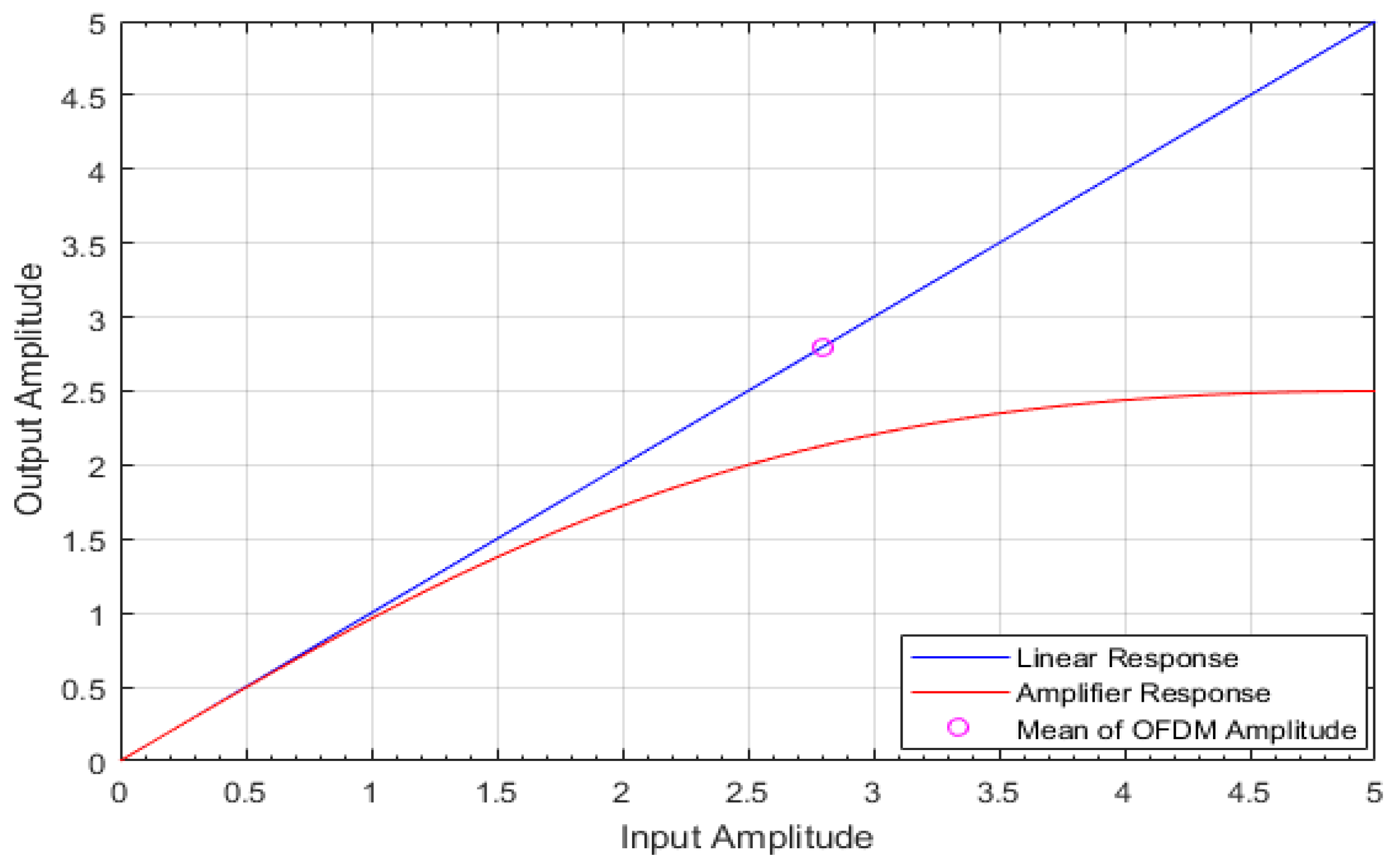
2.2. Clipping

Before amplification through the PA, the signal is clipped as per saturation levels of the PA. The operation of clipping is defined mathematically as

$$x_c^p[n]=\{\begin{array}{c}-A,x^p\\ x^p[n],\\ A,\end{array}\begin{array}{c}{x}^p[n]\le -A\\ \left|x^p[n]\right|<A\\ x^p[n]\ge A\end{array}$$

(11)

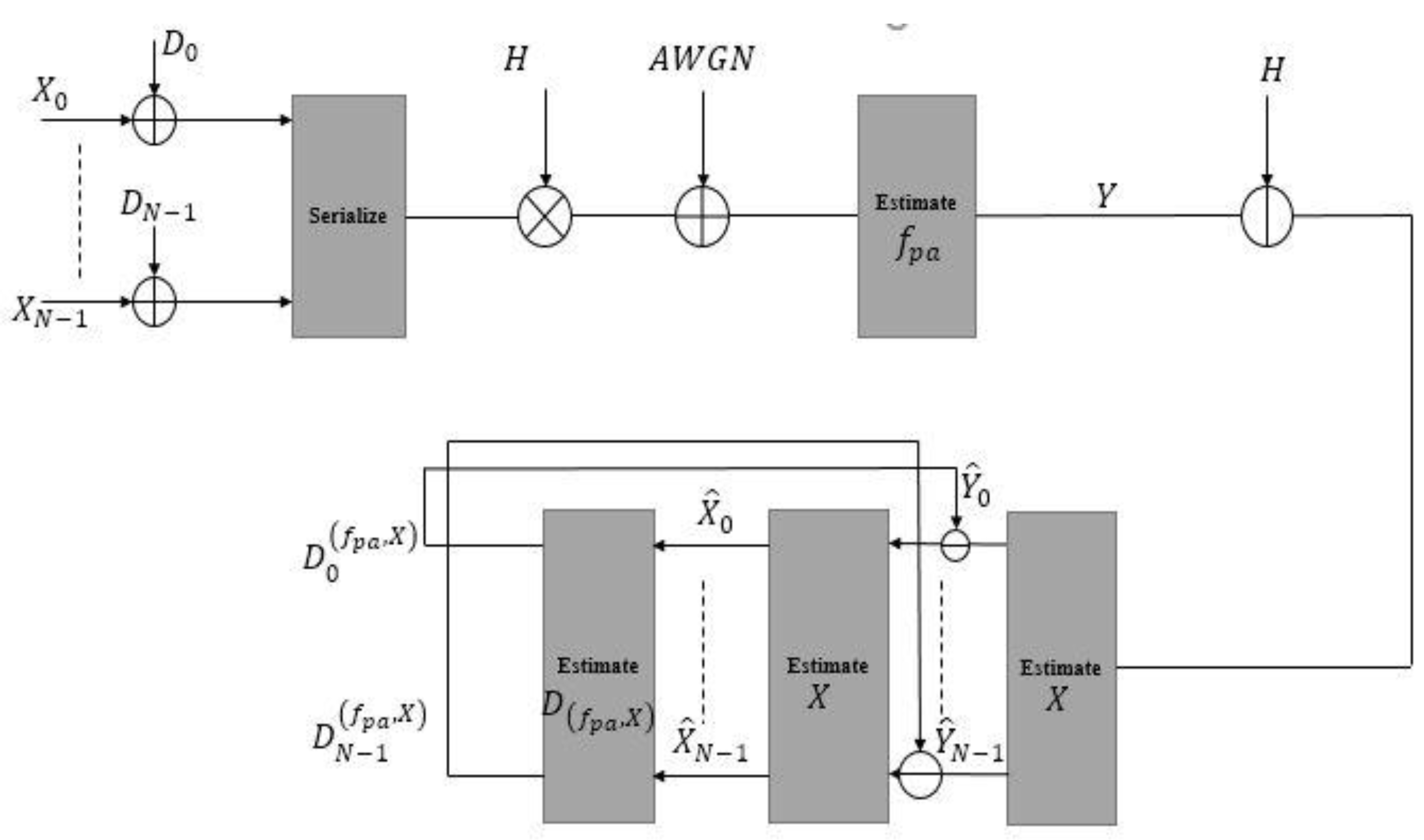
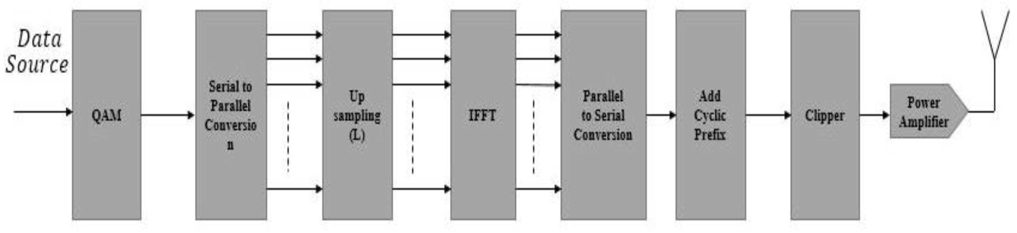
The system model shown in Figure 1 is explained mathematically in the above equations. Here, $x_c^p\left[n\right]$ represents the clipped signal for the $p^{th}$ OFDM signal; "A" determines the level of clipping amplitude level. Clipping is the most basic reduction technique for reducing PAPRs. However, it has a major drawback of in-band and out-band distortion, which causes the performance of the BER in the overall system. When we clip the input signal to the PA, we should make sure that the signal is passing through a linear amplification region so that PAPR performance is improved.

2.3. OFDM Receiver Model

The receiver block comprises the learning PA model, removal of cyclic prefix, then the use of FFT for demodulating the symbols, which is followed by channel equalization. During the start of communication, learning the PA model is necessary. The learned PA model should be updated at some specific intervals. In this work, we have not studied the time frames when the PA model should relearn; it is an optimization proposal. The learning PA model depends upon the frame time, call duration and data rate. The next segment in the receiver model is a distortion-removal block, as shown in Figure 2. In this portion, we used a signal processing algorithm for distortion removal, which is caused by the PAPR. After distortion removal, the parallel stream of the signal is obtained before being downsampled by factor L. The last part describes the unmapping or demodulation of the QAM symbols.

2.4. Learning the Power Amplifier with Neural Network

In this article, firstly, we conducted research to reduce the PAPR in underwater acoustic OFDM communication. Secondly, unnecessary distortion, which is caused by high PAPR, was reduced at the receiver. It affects the BER performance of the overall system; for this, we need to learn the PA model at the receiver. To learn a model we need to train the Machine learning algorithm with a proper set of data. At the beginning of this communication, a set of QAM symbols is generated by the transmitting transducer with different amplitudes over the range of PA characteristics. The data are transmitted through a noisy underwater acoustic BELLHOP Gaussian beam tracking model with several delays and multipath effects. The PA machine learning model at the receiver side is explicated in Figure 2. Hence, at the receiver’s data acquisition, this model is used. If there are better and more appropriate data sets, one can use various deep learning algorithms and train the model before using this distortion mitigation process. Here, we have implemented a neural network (nonparametric) model.

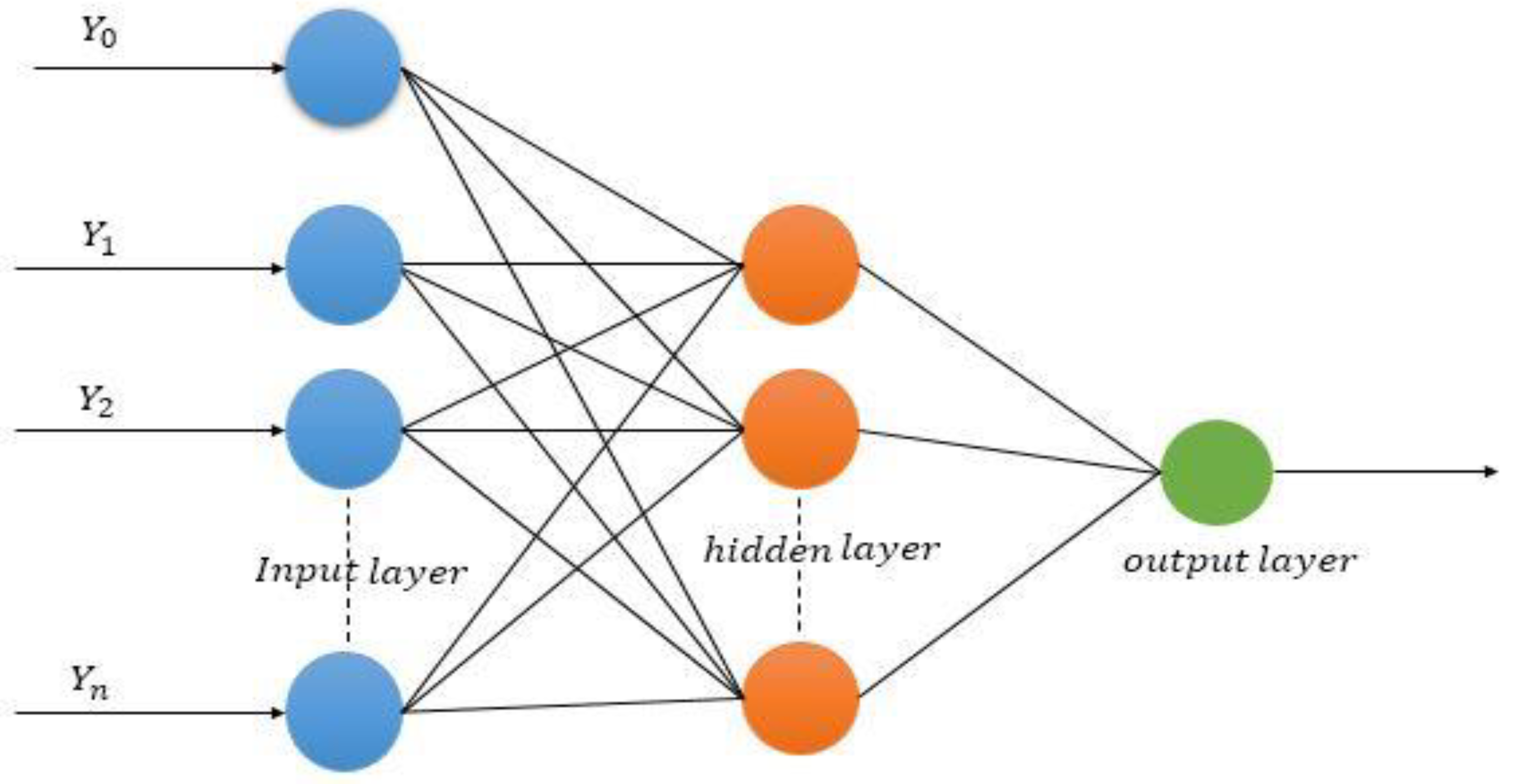
The neural networks are being classified under the nonparametric models. The weight of the hidden neurons that is learned does not provide physical meaning for the undergoing consideration of the problem. The main aim of training a neural network is to estimate the whole function, not only approximating the weights (as in the parametric model). The proposed distortion algorithm demands the knowledge of the PA model at the transmitter side. In this paper, we implement a feed-forward machine learning (neural network) method that estimates the PA characteristics model at the receiver side. A neural network has the advantage of using the method as a universal appropriator. It can realize an arbitrary mapping of a single vector space onto different vector spaces. The training process is regarded as the leaning of weights; supervised and unsupervised are the two types of training processes. The supervised training process is used when the NN knows the output, and it adjusts the weights accordingly. An example is a feed-forward network. In the unsupervised training process, the NN does not know about the output; it recognizes a random pattern and develops a certain relationship. The multilayer feed-forward neural network (MLFNN) is used in this article as we know about the desired output values. Hence, it is the correct decision.

The neurons are ordered as input, hidden, and output layers in a MLFNN, as shown in Figure 3. In each layer, the neurons relate to another neuron in the upcoming layer. There is a connection between $i^{th}$ and $j^{th}$ neuron, which is characterized by $w_{ij}$ and threshold coefficients of ${\vartheta }_i$ and ${\vartheta }_j$, as described in Figure 4. The importance of the neuron is represented by weights that have a connection in the model. We can calculate the outvalue of the neuron as

$$y_j=f({\xi }_j)$$

(12)

$${\xi }_j={\vartheta }_j+{\displaystyle \sum _{i\epsilon {\mathsf{\Gamma }}_j^{-1}}{\omega }_{ji}{y}_i}$$

(13)

In Equation (12), ${\xi }_j$ denotes the potential of the $i^{th}$ neuron function $f({\xi }_i)$ or the transfer function. The transfer function is applied to all neurons $i^{th}$, the transferring signal to the $j^{th}$ neuron. The threshold coefficient is the weight coefficient of the connection between i neuron, where y_i = 1; it is called bias. Then this transfer function can be a sigmoid, defining a nonlinear solution.

$$f({\xi }_i)=\frac{1}{1+e^{-{\xi }_i}}$$

(14)

The threshold ${\vartheta }_j$ and weight $w_{ji}$ coefficients are changed to reduce the sum of the square difference between the actual and desired outputs. After this, the minimum cost function can be written as

$$Q={\displaystyle \sum _j{(y_j-{\widehat{y}}_j)}^2}$$

(15)

The desired output and actual output runs overall j are denoted by vector $y_j$ and ${\widehat{y}}_j$. There is a different training algorithm described for calculating the weight and threshold values in different researches. The most common algorithm is the backpropagation algorithm.

3. Frequentative Decision Feedback (FFB)

In this section, an iterative feedback system is used to remove the distortion in the overall system. It is assumed that the nonlinearity caused by the transmitting side will be mitigated at the receiving side. Figure 5 shows the FFB model used in this paper. If the nonlinearity is present in the discrete time domain, then this analysis provides authentic results. When there is nonlinearity in the continuous time domain, then it gives us approximate results. It can be more accurate when oversampling takes care of the spectral regrowth.

$$\begin{array}{l}{x}_{\frac{n}{L}}^{f_{pa}}=f_{pa(x\frac{n}{L})}\\ \alpha .x\frac{n}{L}+{\widehat{d}}_n{}^{(X)}\end{array}$$

(16)

where x_n represents the input to a PA, f_pa is the learned model for the PA, and oversampling is given as L. The output can be expressed as a linear combination of actual amplified input to the PA and a distortion term. MSE $E\left[{\left|f_{pa}(x\frac{n}{L})-\alpha \cdot x\frac{n}{L}\right|}^2\right]$ is minimized when we put the value of the constant α in such a manner. The variable contains some distorted energy that is not related to $x\frac{n}{L}$. The soft limiter and SSPA nonlinearity are proved $\alpha \to 1$ by putting the value of clipping > 7.3 dB. If the intersymbol interference (ISI) of the channel is less than the value of the cyclic prefix (CP), then it is shortened to a single multicarrier symbol. After this, the distortion looks like the deterministic function of $x\frac{n}{L}$, so ${\widehat{d}}_n^{(X)}$. Hence, the QAM vector will have the $p^{th}$ symbol and $X_L^P$, which will contain the nonlinearity distortion. The FFT can be computed from Equation (16) over the whole interval, which also includes the oversampling discrete interval. Mathematically it is written as follows:

$$FFT\left(x_{\frac{n}{L}}^{f_{pa,p}}\right)=X_L^{f_{pa,p}}=X_L^m+D_L^{(f_{pa,X}{}^p)}$$

(17)

The time index here is K. Then, we can expand Equation (17) further as

$$FFT\left(x_{\frac{n}{L}}^{f_{pa,p}}\right)=\{\begin{array}{c}{X}_k^m,k+D_{L,k}^{(f_{pa,}{X}^p)},k=0,\dots .,\frac{N}{2}-1\\ D_{(L,k)}^{(f_{pa,}{X}^P)},k=\frac{N}{2},\dots .,NL-\frac{N}{2}-1\\ X_{k-N(L-1)}^m+D_{L,k}^{(f_{pa,}{X}^p)},k=NL-\frac{N}{2}-1,\dots .,NL-1.\end{array}$$

Here, $D_{L,k}^{(f_{pa,}{X}^p)},k=\frac{N}{2},\dots .,NL-\frac{N}{2}-1$ is the out-of-band distortion; thus, to minimize this distortion, we use clipping and windowing. The symbol index p will be eliminated with oversampling L for the receiver design to be explained more clearly, which makes equation representation simpler. Furthermore, an assumption takes place before applying a reduction algorithm; the out-of-band distortion is minimized. If $H_k$ is the FFT of the channel impulse response h[n], then, in this regard, the received symbols can be represented as

$$Y_k^{f_{pa}}=H_k(X_k+D_k^{(f_{pa},X)})+Nois{e}_k$$

(18)

where $Nois{e}_k$ is the Additive white guassian noise (AWGN) component for the $k^{th}$ OFDM symbol. A maximum-likelihood receiver for estimating $X$ will be

$$\widehat{X}=\arg \underset{\forall \overline{X}}{\min }{\displaystyle \sum _{k=0}^{N-1}(H_k({\overline{X}}_{k+}{D}_k^{(f_{pa},\overline{X})})-Y_k^{f_{pa}})}$$

(19)

While considering one OFDM symbol, Equation (19) can be written as a vector form. $\overline{X}$ is the transmit symbol vector.

$$\widehat{X}=\arg \underset{\overline{X}}{\min }{\Vert (H\times (\overline{X}+D^{(f_{pa},\overline{X})})-Y^{f_{pa}})\Vert }^2$$

(20)

The element-to-element vector product is denoted by ×. Replacing the value of $Y^{f_{pa}}$ from Equation (18), we can write Equation (20) as

$$\widehat{X}=\arg \underset{\overline{X}}{\min }{\Vert H\times (\overline{X}+D^{(f_{pa},\overline{X})})-H\times (X+D^{(f_{pa},X)})-Noise\Vert }^2$$

(21)

If we solve Equation (21) directly for $D^{(f_{pa},\overline{X})}$, it will lead to exponential complexity as we know $D^{(f_{pa},\overline{X})}$ and $D^{(f_{pa},X)}$ are complex nonlinear functions. Hence, to get the solution, the term $D^{(f_{pa},\overline{X})}$ will not be computed; instead, we assume $D^{(f_{pa},\overline{X})}$, which is not related to X, and it is approximated as an AWGN. Thus, we can write mathematically for N independent subchannels after reducing an ISI channel

$$Y_k^{f_{pa}}=H_k{X}_k+Nois{e}_k$$

(22)

where

$$N\widehat{o}is{e}_k=H_k{D}^{(f_{pa,}X)}+Nois{e}_k$$

(23)

If the receiver computes the value of $D^{(f_{pa},X)}$, the maximum-likelihood problem of Equation (21) will be simplified as

$$\widehat{X}=\arg \underset{\overline{X}}{\min }{\Vert H\times \overline{X}-H\times X-Noise\Vert }^2$$

(24)

From the Equations (22), (23), and (24), regarding computation and complexity, we can deduce the problem as a standard linear solution maximum likelihood decoder. When the transmission is uncoded, the problem of a vector into different N scalar maximum likelihood equations can be reduced as

$${\widehat{X}}_k=\arg \underset{{\overline{X}}_k}{\min }{\Vert H_k\times {\overline{X}}_k-H_K\times X_k-Nois{e}_k\Vert }^2$$

(25)

or it can be written as

$$\widehat{X}=\arg \underset{\overline{X}}{\min }{(H\times [{\overline{X}}_k-\frac{Y_k^{f_{pa}}}{H_k}+D^{(f_{pa,}X)}])}^2$$

(26)

If the value $D^{(f_{pa},X)}$ is known to the receiver, it will select the symbol which is close to $\frac{Y_k^{f_{pa}}}{H_k}-D^{(f_{pa,}X)}$. At the same time, the new system is introduced here with less complexity, and the distortion is reduced.

In Algorithm 1, if the receiver knows the nonlinear PA function $f_{pa}(.)$, then this algorithm can iteratively approximate the distortion term from the received vector $Y^{f_{pa}}$, and it can estimate the QAM vector. This is assuming that the information about the channel and the PA nonlinear model is perfectly known at the receiver. Then, this algorithm can be easily implemented in a few basic steps, as can be seen from Algorithm 1.

Algorithm 1. Frequentative Decision Feedback (FFB).

1: Need: Received $\left[1,\dots .,X_m^{rx}\right]:$ OFDM symbol blocks

2: Make Sure: $H:$ The Channel impulse response is known at the receiver

3: Make Sure: $f_{pa}:$ The PA nonlinear model should be estimated using Machine Learning

4: Procedure Distortion Based Reduction Algorithm

5:  For i do number of OFDM symbols

6:  $X_n\leftarrow$ removed cyclic prefix from $X_m^{rx}$

7:   for j do number of frequentative feedbacks $X_q=((1/sqrt(N)\ast FFT([1,\dots .,X_n]))./H-D^{(f_{pa},X_{n-1})}⊳X_q$     the estimated OFDM symbols, $D^{(f_{pa,X_{n-1}})}$ is the distortion,

8:    $x_n=IFFT\left(X_q\right)$

9:    $x_{n\_amplitude}=absolute\left(x_n\right)$

10:     $x_{n\_phase}=angle\left(x_n\right)$

11:     $Distortio{n}_{temp\_cartesion}=D_{temp\cdot }*\exp \left(sqrt\left(-1\right)*x_{n\_phase}\right)$

12:     $D^{\left(fpa,Xn\right)}=FFT\left(D_{temp\_cartersian}\right)$

13:     $D^{\left(fpa,X_{n-1}\right)}=D^{\left(f_{pa},x_n\right)}$

14:   end for return $X_q$

15:  end for

16: end procedure

4. Results and Discussions

In this section, the results are discussed for the proposed FFB algorithm. We have considered the nonlinearity distortion due to clipping and the TFNN method; keeping information of the acoustic channel is known at the receiver. We trained the data over high SNRs (20dB- 25dB); so to have a less noisy training data. MATLAB version 2017a was used for simulation purposes. The first important block at the receiver side is to estimate the proposed PA model. Additionally, the algorithm is evaluated in the least estimation time, and the BER should show improvement in the nonalgorithm case. There is a different machine learning algorithm that can be used to design PAs if the data is available. The key parameters that should be considered while implementing the machine learning algorithm are training time, amount of data available, acceptable training errors, and validation errors. The simulation parameters are given in

Table 1. Simulation system parameters.

NO.	Parameter	Data
1	Sampling frequency	100 kHz
2	Bandwidth	6.25 kHz
3	FFT points	8192
4	OFDM symbol number	23
5	Number of subcarriers	512
6	Cyclic prefix time	25ms
7	Modulation	64-QAM
8	Sound speed	1500 m/s
9	PA Saturation Level	7.0
10	Signal Clipping	± 7

.

The parameters given in

Table 2. Bellhop channel configuration.

Parameters	Surface Height (m)	Transmitting Side Depth, TX (m)	Receiving Side Depth, RX (m)	Distance between TX and RX (km)	Frequency Range (kHz)
Data	100	30	50	2	10–12

are the bellhop channel configuration for simulation, adopting QAM modulation. A shallow water bellhop channel is generated by MATLAB, assuming the total depth of water is 100 m, with a horizontal range of 2 km. The depth of the transducer is 30 m simultaneously; the depth of the hydrophone is kept at 50 m. Figure 6 shows the ideal SSPA model used in transmitting transducer; it is compared with the exact linear PA model. As mentioned in our proposed (FFB) model, the choice of SSPA is explained from the real scenario, namely, the fact that SSPA nonlinearity can be approximated from Equation (16), which is the summation of linear and nonlinear values. The saturation level is kept around 7 dB in simulation, which is higher than the transmit out voltage. The distortion, which is created by the PAPR, helps us to analyze the effectiveness of the algorithm being researched. The machine learning algorithm is taken to learn the model. We mention the algorithm above as Algorithm 1. It is essential to compare the results between the learned model and the ideal one in terms of learning time and accuracy at the transmitter for the FFB algorithm to achieve constructive results.

4.1. PAPR Performance and Bellhop Channel Impulse Response

The PAPR performance is evaluated with the help of a complementary cumulative distribution function (CCDF) for the proposed model in this section. The PAPR is compared between the addition of clipping and without clipping. It is observed that the proposed method can reduce the PAPR, although this proposed FFB method is a receiver-based PAPR distortion mitigation technique. The reason for adding a clipping block is to verify the performance of the proposed scheme with clipping. In Figure 7, the blue curve is the original OFDM signal. The red line shows the PAPR reduction with the TFNN method; similarly, the green and yellow lines represent the PAPR reductions with and without clipping, respectively. The PAPR is reduced from 11.2 (original) to 7.6 dB for the proposed scheme 64-QAM constellation used at 10^-3 CCDF, as shown in the brown curve. It can be observed from Figure 7 that the FFB model performs significantly better by adding clipping and in comparison to the TFNN method, i.e., 8.1 dB. However, the computational complexity is lower in the proposed neural network deep learning model.

Figure 8 illustrates the impulse response of the channel at 2 km, which is based on the sound speed profile used in the simulation. The sound speed was saved in the range of 1480 to 1500 m/s. The time delay can be observed in the figure with the normalized amplitude.

4.2. Performance Evaluation of Neural Network and Bit Error Rate

In this implementation, the data set of 2000 × 612, having subcarriers 512 with 100 cyclic prefixes, is shaped again into smaller sets of data. In this way, the six data scalar inputs are added to the neural network. Here, the subcarriers received are 612. The software uses only 516. Then, we form the 2000 × 512 data set matrix into smaller sets. For example, 25,800 × 600 data sets will have 300 OFDM symbols, which are evaluated as 25,800 × 6/516 = 300, as shown in

Table 3. Learning algorithm.

Training Algorithm	Data Required	Training Time	Fit Goodness
Levenberg–Marquardt	25,800 × 6 * Number of OFDM symbols = 300	16.59 s	MSE: 0.00138 at 93 frequentatives. Data Division Random

* it relates to the column "25800*6 Number of OFDM symbols = 300.

. For better estimation of the PA model, the data which have been fed to neurons are important with regard to quality and quantity. When implementing the neural network, only one hidden layer is used with 12 neurons, which has six input and six output neurons. The sigmoid transfer function is used to define neurons. If we add another hidden layer that has enough numbers of neurons, this will fit any finite input and output problem. Increasing the number of neurons will demand more training time and computation capability. As we know, the received OFDM symbols $X$ used for training the proposed PA model are not dependent. Therefore, we can reduce the number of inputs in the neural network. In contrast, the number of neurons at the input is less than the length of OFDM symbols. By doing this, the convergence becomes a lot faster and more accessible when learning the relationship between 6 rather than 612 input symbols (in this simulation, the OFDM symbol length was 612). In a feature vector, the actual number of neurons is the same as the columns in a neural network. Here, we have reshaped the feature vector from 612 to 6. Hence, the computational complexity is reduced. We selected the number 6 for simulation. It is possible to choose a different number of less than 10 feature vectors for evaluating and analyzing the performance of this model. The bad estimation was observed beyond the PA saturation region when the number of hidden neurons was less than 12. Therefore, we studied the algorithm results and simulated the whole NN with 12 hidden neurons. The learning algorithm is shown in Table 3.

The performance of the FFB algorithm was analyzed when the distortion was only due to the PA, and distortion was also verified with the signal clipping. Let us show how the BER reduces when we apply FFB to the overall OFDM system, with and without clipping. For this case, we used the simulation parameters given in Table 1. In Figure 9, the blue line shows the BER curve without applying clipping and the FFB algorithm. At the same time, the BER curve (red line) is shown for the TFNN method. By adding the clipping, there is an improvement in the BER performance with the FFB algorithm; it can be seen in the green and yellow lines. The nonlinearity distortion is caused by a PA when it gets into a saturation region. From Figure 9, the proposed FFB algorithm outperforms the rest when it is trained with the neural network. The neural network gives us the best result at all SNRs above 10 dB.

4.3. QAM Scattering Plots

From Figure 10 and Figure 11, the QAM symbols can be seen at the receiver before and after applying the FFB algorithm. We are able to understand how good the algorithm works after analyzing both scattered plots. In Figure 10, the 64 QAM symbols are received at 20 dB SNR, and the algorithm is not applied. From Figure 11, the QAM received symbols are shown after a noisy underwater acoustic channel with the application of the FFB algorithm. It is found that if the FFB algorithm is not applied, many of the received symbols are out of the QAM coordinates. The proposed algorithm reduces the unnecessary noise to a more significant extent, as can be observed in Figure 11. Here all QAM symbols are within the decision coordinates for a specific symbol’s alphabets. It is proved that the QAM symbols with no PAPR reduction algorithm (FFB) are noisier than the ones with FFB applied. After comparing both pictures, it is noticeable that many symbols in Figure 10 are scattered out of the 64 quadrants. In the case of FFB, almost all the QAM symbols are near the quadrature. Thus, it can be demodulated with less error and results in a decrease in BERs.

Next, the variation in BERs is analyzed at different PA saturation levels when the distortion is due to PA nonlinearity, which is the same as the BER variation with clipping and PA nonlinearity. If the PA saturation levels are increased, the BER decreases. It can be justified as an increase in the saturation level leads to an enhancement in the linear operation range of the PA. Figure 12 exhibits the change in BER performance with PA saturation levels of 10, 7, and 5 dB. It is clear from Figure 12 that the BER is lowest at the 10 dB saturation level compared with other levels.

5. Conclusions and Future Work

This paper presents the machine learning algorithm for reducing the BER in UWA OFDM communication systems with a reduction in PAPR. An OFDM system is considered by adding clippers in a communication system, which reduces the PAPR but creates nonlinearity distortion caused by the PA. The proposed FFB method estimates the PA nonlinearity at the receiver with the help of a modern machine learning algorithm. The deep learning method gives us a feasible estimation of the data. The DPD technique is very difficult to implement because most of the underwater acoustic transceivers consume very high energy. In such conditions, one can use this algorithm to reduce the PAPR. Reliable communication can be achieved if the FFB algorithm is performed at both sides of the base station and UWA OFDM modems. The results prove that modern machine learning algorithms can be used in signal processing and communication engineering for reducing distortion, which is caused by high PAPRs in OFDM systems. In future work, the number of neurons can be reduced with more hidden layers and less input–output neurons, and the time frame can be estimated in order to maintain lower BERs.

References

1. Tianzeng, X.; Lufen, X. Chapter 1- Introduction, Digital Underwater Acoustic Communications; Xu, T., Xu, L., Eds.; Academic Press: New York, NY, USA; pp. 1–30.
2. Yuri Labrador, M.K.; Deng, P.; Jerry, M. Modulation and error correction in the underwater acoustic communication channel. Int. J. Comput. Sci. Netw. Secur. 2009, 9, 123–130. [Google Scholar]
3. Zhou, S.; Wang, Z. OFDM for Underwater Acoustic Communications; Wiley Publishing: Hoboken, NJ, USA, June 2014; pp. 1–22. [Google Scholar]
4. Abd El-Galil, M.S.; Soliman, N.F.; Abdalla, M.I.; Abd El-Samie, F.E. Efficient underwater acoustic communication with peak-to-average power ratio reduction and channel equalization. Int. J. Speech Technol. 2019, 22, 649–696. [Google Scholar] [CrossRef]
5. Wu, J.; Ma, X.; Qi, X.; Babar, Z.; Zheng, W. Influence of pulse shaping filters on PAPR performance of underwater 5G communication system technique: GFDM. Wirel. Commun. Mob. Comput. 2017, 2017, 4361589. [Google Scholar] [CrossRef] [Green Version]
6. Lee, B.M.; Rim, Y.S.; Noh, W. A combination of selected mapping and clipping to increase energy efficiency of OFDM systems. PLoS ONE 2017, 12, e0185965. [Google Scholar] [CrossRef] [PubMed] [Green Version]
7. D’Andrea, A.N.; Lottici, V.; Reggiannini, R. Nonlinear predistortion of OFDM signals over Frequency-selective fading channels. IEEE Trans. Commun. 2001, 49, 837–843. [Google Scholar] [CrossRef]
8. Gomathi, R.M.; Martin Leo Manickam, J. PAPR reduction technique using combined DCT and LDPC based OFDM system for underwater acoustic communication. ARPN J. Eng. Appl. Sci. 2016, 11, 4424–4430. [Google Scholar]
9. Wunder, G.; Fischer, R.F.H.; Boche, H.; Litsyn, S.; No, J.-S. The PAPR problem in OFDM transmission: New directions for a long-lasting problem. IEEE Signal Process. Mag. 2013, 30, 130–144. [Google Scholar] [CrossRef] [Green Version]
10. Raza, W.; Ma, X.; Ali, A.; Shah, Z.A.; Mehdi, G. An implementation of partial transmit sequences to design energy efficient underwater acoustic OFDM communication system. Int. J. Comput. Sci. Inf. Secur. (IJCSIS) 2020, 18, 19–26. [Google Scholar]
11. Li, L.; Tellambura, C.; Tang, X. Improved tone reservation method based on deep learning for PAPR reduction in OFDM system. In Proceedings of the 11th International Conference on Wireless Communications and Signal Processing (WCSP), Xi’an, China, 23 October 2019. [Google Scholar]
12. Zhang, M.; Liu, M.; Zhong, Z. Neural network assisted active constellation extension for PAPR reduction of OFDM system. In Proceedings of the 11th International Conference on Wireless Communications and Signal Processing (WCSP), Xi’an, China, 23 October 2019. [Google Scholar]
13. Wada, T.; Toma, T.; Dawodi, M.; Baktash, J. A Denoising Autoencoder based wireless channel transfer function estimator for OFDM communication system. In Proceedings of the 2019 International Conference on Artificial Intelligence in Information and Communication (ICAIIC0), Okinawa, Japan, 11 February 2019. [Google Scholar]
14. Tellado, J.; Hoo, L.M.C.; Cioffi, J.M. Maximum-likelihood detection of nonlinearly distorted multicarrier symbols by iterative decoding. IEEE Trans. Commun. 2003, 51, 218–228. [Google Scholar] [CrossRef]
15. ROWE, H.E. Memoryless nonlinearities With gaussian inputs: Elementary results. Bell Syst. Tech. J. 1982, 61, 1519–1525. [Google Scholar] [CrossRef]
16. D’Andrea, A.N.; Lottici, V.; Reggiannini, R. RF power amplifier linearization through amplitude and phase predistortion. IEEE Trans. Commun. 1996, 44, 1477–1484. [Google Scholar] [CrossRef]
17. Yao, Y.C.; Hung, H.L.; Wen, J.H. PAPR reduction in OFDM system using differential evolution-based partial transmit sequences scheme. In Proceedings of the 2011 International Conference on Machine Learning and Cybernetics, Guilin, China, 10 July 2011. [Google Scholar]
18. Hasan, A.N.; Shongwe, T. Proposed Machine learning system to predict and estimate impulse noise in OFDM communication system. In Proceedings of the IECON 2016-42nd Annual Conference of the IEEE Industrial Electronics Society, Florence, Italy, 23 October 2016. [Google Scholar]
19. Chackochan, R.; Soni, H. Peak to average power ratio (PAPR) reduction in OFDM for a wlan network Using SLM technique. In Proceedings of the 2011 3rd International Conference on Electronics Computer Technology, Kanyakumari, India, 7 July 2011. [Google Scholar]
20. Güner, A.; Alçin, Ö.F. Analysis of complex extreme learning machinebased nonlinear equalizer for coherent optical OFDM systems. In Proceedings of the 2017 International Artificial Intelligence and Data Processing Symposium (IDAP), Malatya, Turkey, 16 September 2017. [Google Scholar]
21. Marsalek, R.; Jardin, P.; Baudoin, G. From post-distortion to pre-distortion for power amplifiers linearization. IEEE Commun. Lett. 2003, 7, 308–310. [Google Scholar] [CrossRef]
22. Ye, H.; Li, G.Y.; Juang, B.-H. Power of deep learning for channel Estimation and signal detection in OFDM systems. IEEE Wirel. Commun. Lett. 2018, 7, 114–117. [Google Scholar] [CrossRef]
23. Adel, A.M.; Saleh, S.M. Frequency-independent and frequency-dependent nonlinear models of TWT amplifiers. IEEE Trans. Commun. 1981, 29, 1715–1720. [Google Scholar]
24. Sohn, I. A low complexity PAPR reduction scheme for OFDM systems via neural networks. IEEE Commun. Lett. 2014, 18, 225–228. [Google Scholar] [CrossRef]
25. Kim, M.; Lee, W.; Cho, D.-H. A novel PAPR reduction scheme for OFDM system based on deep learning. IEEE Commun. Lett. 2018, 22, 510–513. [Google Scholar] [CrossRef]
26. Zhang, J.; Cao, Y.; Han, G.; Fu, X. Deep neural network-based underwater OFDM receiver. IET Commun. 2019, 13, 1998–2002. [Google Scholar] [CrossRef]
27. Zhang, Y.; Li, J.; Zakharov, Y.; Li, X.; Li, J. Deep learning based underwater acoustic OFDM communications. Appl. Acous. 2019, 154, 53–58. [Google Scholar] [CrossRef]
28. Giacoumidis, E.; Tomkos, I.; Tang, J.M. Adaptive modulation-induced reduction in filter concatenation impairment for optical OFDM metro/regional systems. J. Opt. Commun. Netw. 2011, 3. [Google Scholar] [CrossRef]
29. Giacoumidis, E.; Jin, X.Q.; Tsokanos, A.; Tang, J.M. Statistical performance comparisons of optical OFDM adaptive loading algorithms in multimode fiber-based transmission systems. IEEE Photonics J. 2010, 2, 1051–1059. [Google Scholar] [CrossRef]
30. Li, X.; Cimini, L.J. Effects of clipping and filtering on the performance of OFDM. IEEE Commun. Lett. 1998, 3, 34–38. [Google Scholar]
31. Wu, J. Iterative compressive sensing for the cancellation of clipping noise in underwater acoustic OFDM system. Wirel. Pers. Commun. 2018, 103, 2093–2107. [Google Scholar] [CrossRef]
32. Deutsche Telekom, A.G. On the Degradation of OFDM-Signals due to Peak-Clipping in Optimally Predistorted Power Amplifiers; Research Center: Darmstadt, Germany, 1998. [Google Scholar]
33. Gregorio, F.H.; Werner, S.; Cousseau, J.; Figueroa, J.; Wichman, R. Receiver-side nonlinearities mitigation using an extended iterative decision-based technique. Signal Process. 2011, 91, 2042–2056. [Google Scholar] [CrossRef]
Figure 1. OFDM (orthogonal frequency divisional multiplexing) transmit blocks with clipping.
Applsci 10 04986 g001
Figure 2. The framework of the OFDM receiver.
Applsci 10 04986 g002
Figure 3. Generic neural network composed of three layers.
Applsci 10 04986 g003
Figure 4. The connection between neurons.
Applsci 10 04986 g004
Figure 5. Frequentative decision feedback (FFB) model.
Applsci 10 04986 g005
Figure 6. Power amplifier (PA) solid-state model used at the transmitter.
Applsci 10 04986 g006
Figure 7. Complementary cumulative distribution function (CCDF) of PAPR performance for proposed and conventional schemes.
Applsci 10 04986 g007
Figure 8. Simulation result of the channel impulse response.
Applsci 10 04986 g008
Figure 9. Bit error rate (BER) vs. SNR for the FFB algorithm.
Applsci 10 04986 g009
Figure 10. QAM scatter plot received symbols without FFB. Distortion due to clipping with PA model.
Applsci 10 04986 g010
Figure 11. QAM scatter plot received symbols with FFB. Distortion due to clipping with PA model.
Applsci 10 04986 g011
Figure 12. Bit error rate vs. SNR for FFB, distortion with PA nonlinearity and PA saturation levels of 10, 7, and 5 dB.
Applsci 10 04986 g012