Model Updating Using Frequency Response Functions Based on Sherman–Morrison Formula

Abstract

Model updating plays an important role in dynamics modeling with high accuracy, which is widely used in mechanical engineering. In this paper, a model updating method using frequency response function (FRF) is proposed based on Sherman–Morrison formula, in which only the initial FRFs and parameter perturbations are employed to calculate the sensitivity avoiding repeated finite element (FE) analyses and improving the computational efficiency. Firstly, the sensitivity of FRFs to the design parameters is calculated by Sherman–Morrison formula based on the QR decomposition of the system dynamic stiffness matrix variation after parameter perturbations, then the influence of damping on the amplitude of FRFs is considered to select an appropriate frequency range, and finally conduct the model updating according to the sensitivity of the FRFs. By employing simulation examples of a truss and a solar wing and the experiment of an aluminum frame, the updating error is still within ±1.00% in the condition of 5% random white noise, which shows the proposed method has high accuracy and a certain anti-noise capability. When only a few numbers of frequency points are selected near the resonance peak of the FRFs, the result shows that selecting the appropriate frequency range and points can reduce the computational cost. The results of the experiment study show that the proposed method can effectively identify the structural parameters. The above results verify the feasibility and effectiveness of proposed model updating method using FRFs.

1. Introduction

Finite element model with high accuracy plays an important role in structural dynamics design, which is the premise of dynamic response prediction, vibration control, and structural optimization [1,2,3]. Due to the idealization hypothesis of structural simplification, the errors of structural parameters, and the errors of finite element (FE) discretization, the FE models may not accurately reflect the dynamics performance of the structures [4,5,6]. With the rapid development of numerical simulation in engineering applications, model updating methods gradually revealed its importance, which makes the dynamic characteristics of the theoretical model as consistent as possible with the actual structure.

As a bond between FE models and actual structures, model updating has become a powerful tool and which has been paid extensive attention [7,8]. Many types of approaches have been developed for a variety of problems. Shabbir et al. [9] proposed a method based on particle swarm optimization to update the FE model by using sequence niche technology, which greatly improved the reliability of finding the global minimum; Behmanesh et al. [10] proposed a new probabilistic FE model updating method based on hierarchical Bayesian modeling for identification of structural parameters under varying environmental conditions. Taking the strain mode as the target response, Zhan and Guo et al. [11] constructed the target function to be updated by using the strain mode frequency and modal confidence errors, the parameters were updated by using the Genetic Algorithm. Aiming at the model updating of the nonlinear structure, Wang and Ren et al. [12] took the instantaneous characteristics, including instantaneous frequency and instantaneous amplitude, as the objective function of the nonlinear model updating, and used the annealing global optimization method to obtain the optimal value of the nonlinear parameters. Zang et al. [13] proposed a model updating method that separated the non-linear characteristics of subsystem from the parameter uncertainties to establishing a representative linear mathematical model and applied it to a structural dynamics verification problem which developed by Sandia National Laboratory. The above methods focus on the recent hot spots to carry out research, frequency response function (FRF)’s based model updating is an alternative method with some advantages, FRFs can adequately reflect the dynamic characteristics of a structure, using which as the feature will get rid of modal identification.

Model updating based on FRFs avoids the error caused by modal fitting, and match of the predicted modal shapes with the measured data are not necessary, so it is suitable for structural updating with relatively dense modal distribution. Shadan et al. [14,15] proposed a new structural damage detection method based on FRFs data and natural frequencies, adopted pseudo-linear sensitivity equation to accurately identify the location and severity of damage; Esfandiari et al. [16,17] proposed an estimation method for structure mass and stiffness considering damping effect and using the FRF data for FE model updating; Pradhan et al. [18] proposed a FE model updating method that can identify and update the damping matrix of the system, and studied the updating capability of different damping levels through three different experimental beam structures; Li et al. [19] proposed an iterative method combining model updating method with model reduction technology, effectively improved the efficiency of the updating; Hong et al. [20] successfully updated the stiffness, mass and damping parameters between the analytical and the experimental FRFs through the laboratory test of the four-story shear frame structure; Wang et al. [21,22] conducted the model updating of local nonlinear structure based on the initial FE model of the structure and the primary harmonic response data obtained from low amplitude and high amplitude excitation. The above scholars have done a lot of research on the model updating based on FRFs. However, the selection of parameters plays a significant role in the progress of model updating. The sensitivity of the FRFs has great potential for a vibration analysis, which is not involved in the above methods. Reasonable selection of parameters can effectively improve the quality and efficiency of model updating, which is inseparable from the sensitivity analysis of the parameters, so model updating method based on the sensitivity of FRFs has more important significance.

The model updating based on the sensitivity of FRFs attracted wide attention in the early 1990′s [23]. Sipple et al. [24] proposed a new FE model updating method that uses numerical sensitivity instead of analytical sensitivity to solve inverse problems, which does not need model reduction and data extension, and has good robustness, stability and fault tolerance; Weng et al. [25] proposed a new iterative substructuring method to accurately obtain the characteristic solution and characteristic sensitivity of the structure, which is suitable for model updating of large and complex structures; Jiang et al. [26] expressed the thermal dependent elastic constants and thermal expansion coefficients as intermediate function by temperature independent variables, and used the perturbation method to calculate the sensitivity for parameter identification; On the basis of the basic concept of unconstrained optimization problem and three regularization solutions, Mohammad et al. [27] proposed a novel sensitivity based FE model updating method, and simultaneously updated the element mass matrix and stiffness matrix of the FE model; Esfandiari et al. [28] proposed a FE model updating method using incomplete strain data in frequency domain to detect variations in stiffness and mass parameters. The common sensitivity analysis methods using FRFs are the finite difference method [29] or the combined approximations (CAs) method [30]. These methods are based on obtaining the stiffness matrix, damping matrix, and mass matrix of the structures. The disadvantage of these methods is that repeated analysis is required in the process of structural parameter identification, and they are not applicable under the premise of unknown dynamic stiffness matrix. For example, the modal parameters of the structure can be obtained through experiments, but the complete information of the dynamic stiffness matrix is difficult to obtain. The Sherman–Morrison formula was first proposed by Sherman and Morrison and it can be used to represent the varying of matrix; Turan et al. [31] used the Sherman–Morrison formula of singular value decomposition to calculate the optimal perturbation of the sensitivity value of the extreme value and the design variable, thus achieving the response change that is difficult to obtain with the response derivatives; Zhu et al. [32,33,34,35] used the Sherman–Morrison formula for mass elimination of multi-transducers, and the revised FRFs results were in good agreement with the target values.

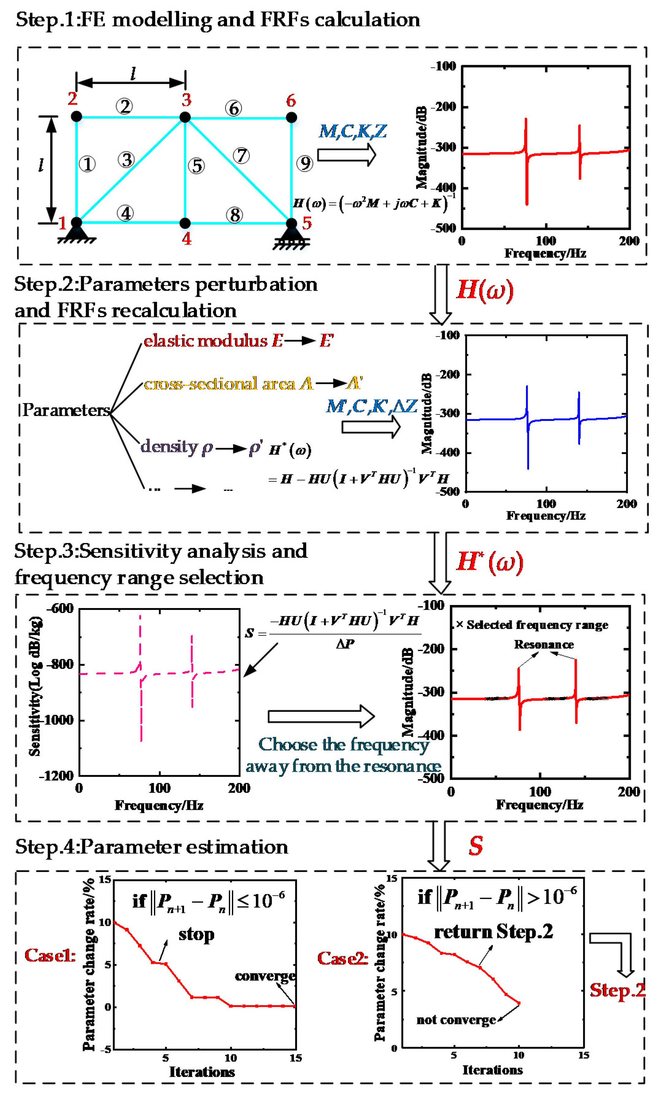
In this study, a model updating method using FRFs based on Sherman–Morrison formula is proposed, only the initial FRFs and parameter perturbations are employed to calculate the sensitivity avoiding repeated FE analyses and calculations, which improves the computational efficiency of model updating. The detail formulation of sensitivity analysis and model updating based on Sherman–Morrison formula is introduced in Section 2, the implementation procedure of the model updating is described in Section 3, and the numerical examples of a planar truss and a solar wing and the experiment of aluminum solar panel frame are used to verify the proposed method in Section 4. The conclusions are summarized in Section 5.

2. Theoretical Analysis

This section verifies that the model updating method using FRFs based on Sherman–Morrison formula can obtain the sensitivity of the FRFs to the parameters only by initial FRFs and parameter perturbations, which can avoid repeated finite element analyses and calculations.

2.1. Sensitivity Analysis Based on SMW

The dynamic equation of the multi-degrees-of-freedom system in the frequency domain can be expressed as

$$\left(-{\omega }^2\mathit{M}+j\omega \mathit{C}+\mathit{K}\right)x\left(\omega \right)=\mathit{F}(\omega )$$

(1)

where M is the mass matrix, K is the stiffness matrix, C is the damping matrix, x(ω) and F(ω) are the Fourier transformation of displacement response and excitation force, respectively.

The dynamic stiffness matrix Z(ω) of the system is

$$\mathit{Z}\left(\omega \right)=-{\omega }^2\mathit{M}+j\omega \mathit{C}+\mathit{K}$$

(2)

The relation between FRFs H(ω) and dynamic stiffness matrix Z(ω) is

$$\mathit{H}\left(\omega \right)={\mathit{Z}}^{-1}\left(\omega \right)$$

(3)

If the FRFs data H(ω) of the system is a function of a design parameter P_m, then the sensitivity S of the FRFs data H(ω) of the system is the first partial derivative of the FRFs with respect to the design parameter is $\frac{\partial \mathit{H}}{\partial {\mathit{P}}_m}$, which be expressed as

$$\mathit{S}=\frac{\partial \mathit{H}}{\partial {\mathit{P}}_m}=-\mathit{H}\frac{\partial \mathit{Z}}{\partial {\mathit{P}}_m}\mathit{H}$$

(4)

According to the formula, the variation of FRFs is the variation of dynamic stiffness. For a specific frequency ω_r, it can be obtained from Equation (4) that the first derivative of dynamic stiffness with respect to a variable P_m is:

$$\frac{\partial \mathit{Z}}{\partial {\mathit{P}}_m}=\left(\frac{\partial \mathit{K}}{\partial {\mathit{P}}_m}+j{\omega }_r\frac{\partial \mathit{C}}{\partial {\mathit{P}}_m}-{\omega }_r{}^2\frac{\partial \mathit{M}}{\partial {\mathit{P}}_m}\right)$$

(5)

Equation (5) can be expressed in differential form as

$$\delta \mathit{Z}=\left(\delta \mathit{K}+j{\omega }_r\delta \mathit{C}-{\omega }_r{}^2\delta \mathit{M}\right)$$

(6)

where δZ, δM, δC, and δK represent the variations of dynamic stiffness matrix, mass matrix, damping matrix, and stiffness matrix, respectively.

However, the damping of the structure is related to the material performance of individual members and the difference of FE modeling. The influence of damping on the FRF amplitude is significant in resonance and decreases rapidly as the damping moves away from resonance. Therefore, the selection of appropriate frequency range can mitigate the impact of damping on the model updating results.

We assume that a system of n-degrees of freedom is subject to mass perturbation δm_i at the ith-degree of freedom, and stiffness perturbation δk_i at the jth-degree of freedom [32], the perturbations of the mass matrix δM and the stiffness matrix δK can be expressed as

$$\delta \mathit{M}=\left[\begin{array}{ccccc}0& \cdots & 0& \cdots & 0\\ ⋮& \ddots & ⋮& ⋮& ⋮\\ 0& ⋮& \delta m_i& ⋮& 0\\ ⋮& ⋮& ⋮& \ddots & ⋮\\ 0& \cdots & 0& \cdots & 0\end{array}\right]$$

(7)

$$\delta \mathit{K}=\left[\begin{array}{ccccc}0& \cdots & 0& \cdots & 0\\ ⋮& \ddots & ⋮& ⋮& ⋮\\ 0& ⋮& \delta k_j& ⋮& 0\\ ⋮& ⋮& ⋮& \ddots & ⋮\\ 0& \cdots & 0& \cdots & 0\end{array}\right]$$

(8)

We can rewrite the perturbations of the mass matrix δM and the stiffness matrix δK as

$$\{\begin{array}{c}\delta \mathit{M}={\mathit{G}}_{uv}{\mathit{G}}_{uv}{}^T\\ \delta \mathit{K}={\mathit{X}}_{uv}{\mathit{X}}_{uv}{}^T\end{array}$$

(9)

Where u and v represent the nodes on each side of the unit. G_uv and X_uv are expressed as

$${\mathit{G}}_{uv}=\sqrt{\delta m_i}\left[\begin{array}{ccccc}0& \cdots & 0& \cdots & 0\\ ⋮& \ddots & ⋮& ⋮& ⋮\\ 0& ⋮& 1& ⋮& 0\\ ⋮& ⋮& ⋮& \ddots & ⋮\\ 0& \cdots & 0& \cdots & 0\end{array}\right]$$

(10)

$${\mathit{X}}_{uv}=\sqrt{\delta k_j}\left[\begin{array}{ccccc}0& \cdots & 0& \cdots & 0\\ ⋮& \ddots & ⋮& ⋮& ⋮\\ 0& ⋮& 1& ⋮& 0\\ ⋮& ⋮& ⋮& \ddots & ⋮\\ 0& \cdots & 0& \cdots & 0\end{array}\right]$$

(11)

Therefore, the variation of the system dynamic stiffness matrix δZ can be expressed as

$$\delta \mathit{Z}=-{\omega }_r{}^2{\mathit{G}}_{uv}{\mathit{G}}_{uv}{}^T+{\mathit{X}}_{uv}{\mathit{X}}_{uv}{}^T$$

(12)

The inverse for the variation of dynamic stiffness matrix δZ which is the variation of FRFs δH is obtained by applying the Sherman–Morrison formula

$$\begin{array}{l}\delta \mathit{H}=\delta {\mathit{Z}}^{-1}={\mathit{H}}^{*}\left({\omega }_r\right)-\mathit{H}\left({\omega }_r\right)\\ =-\mathit{H}\left[\begin{array}{cc}-{\omega }_r{\mathit{G}}_{uv}& {\mathit{X}}_{uv}\end{array}\right]{\mathit{L}}^{-1}\left[\begin{array}{c}{\omega }_r{\mathit{G}}_{uv}{}^T\\ {\mathit{X}}_{uv}{}^T\end{array}\right]\mathit{H}\end{array}$$

(13)

where L is a 2N × 2N matrix given by

$$\mathit{L}=\left[\begin{array}{cc}{\mathit{I}}_{N\times N}-{\omega }_r{}^2{\mathit{G}}_{uv}{}^T\mathit{H}{\mathit{G}}_{uv}& {\omega }_r{\mathit{G}}_{uv}{}^T\mathit{H}{\mathit{X}}_{uv}\\ -{\omega }_r{\mathit{X}}_{uv}{}^T\mathit{H}{\mathit{G}}_{uv}{}^T& {\mathit{I}}_{N\times N}+{\mathit{X}}_{uv}{}^T\mathit{H}{\mathit{X}}_{uv}\end{array}\right]$$

(14)

By substituting Equation (13) into Equation (4), the sensitivity of the FRFs with respect to perturbation parameters can be obtained. Therefore, the sensitivity of FRFs to the perturbation parameters can be directly solved by only the initial FRFs and parameter perturbations to avoid repeated FE analyses and calculations.

The FRFs H*(ω) of the system changed by parameter perturbation can be obtained according to Sherman–Morrison formula:

$$\begin{array}{l}{\mathit{H}}^{*}\left(\omega \right)={\mathit{Z}}^{*}{}^{-1}\left(\omega \right)={\left(\mathit{Z}\left(\omega \right)+\mathrm{\Delta }\mathit{Z}\left(\omega \right)\right)}^{-1}\\ ={\mathit{Z}}^{-1}-{\mathit{Z}}^{-1}\mathit{U}{\left(\mathit{I}+{\mathit{V}}^T{\mathit{Z}}^{-1}\mathit{U}\right)}^{-1}{\mathit{V}}^T{\mathit{Z}}^{-1}\\ =\mathit{H}-\mathit{H}\mathit{U}{\left(\mathit{I}+{\mathit{V}}^T\mathit{H}\mathit{U}\right)}^{-1}{\mathit{V}}^T\mathit{H}\end{array}$$

(15)

Therefore, the sensitivity of FRFs based on Sherman–Morrison formula can be expressed as

$$\mathit{S}=\frac{-\mathit{H}\mathit{U}{\left(\mathit{I}+{\mathit{V}}^T\mathit{H}\mathit{U}\right)}^{-1}{\mathit{V}}^T\mathit{H}}{\mathrm{\Delta }\mathit{P}}$$

(16)

where Z*(ω) is the dynamic stiffness matrix changed by parameter perturbation, ΔZ(ω) is the variation of the dynamic stiffness matrix, which is caused by the change quantity ΔP, and ΔZ(ω) can be decomposed into two matrices U(ω) and V^T(ω), I is the n-order identity matrix.

2.2. Frequency Response Function (FRF)’s Model Updating Based on Sensitivity Analysis

The purpose of the model updating is to minimize the difference of FRFs between the experimental and the FE model. The difference between the FRFs of experimental model H*(ω) and the FRFs of FE model H(ω) are used to construct the objective function as follows:

$$min{\Vert \delta \Vert }^2$$

(17)

$$\delta ={\mathit{H}}^{*}\left(\omega \right)-\mathit{H}\left(\omega \right)$$

(18)

where δ is the difference between the experimental FRFs and the corresponding analysis values, which is called the residual vector.

Equation (4) is rewritten as:

$$\mathit{S}=\frac{\partial \mathit{H}}{\partial {\mathit{P}}_m}=\underset{\mathrm{\Delta }P\to 0}{lim}\frac{\mathrm{\Delta }\mathit{H}\left(\omega \right)}{\mathrm{\Delta }\mathit{P}}=\underset{\mathrm{\Delta }P\to 0}{lim}\left[-{\mathit{H}}^{*}\left(\omega \right)\frac{\mathrm{\Delta }\mathit{Z}}{\mathrm{\Delta }{\mathit{P}}_m}\mathit{H}\left(\omega \right)\right]$$

(19)

and

$$\delta =\mathrm{\Delta }\mathit{H}\left(\omega \right)=-{\mathit{H}}^{*}\left(\omega \right)\left(\mathrm{\Delta }\mathit{K}+j{\omega }_r\mathrm{\Delta }\mathit{C}-{\omega }_r{}^2\mathrm{\Delta }\mathit{M}\right)\mathit{H}\left(\omega \right)$$

(20)

where the changes of the total mass matrix ΔM and the total stiffness matrix ΔK of the structure can be expressed by the sum of partial derivatives of each updating element:

$$\mathrm{\Delta }\mathit{M}={\displaystyle \sum _{i=1}^{nm}\frac{\partial \mathit{M}}{\partial {\mathit{P}}_i^M}}\mathrm{\Delta }{\mathit{P}}_i^M$$

(21)

$$\mathrm{\Delta }\mathit{K}={\displaystyle \sum _{j=1}^{ns}\frac{\partial \mathit{K}}{\partial {\mathit{P}}_j^S}}\mathrm{\Delta }{\mathit{P}}_j^S$$

(22)

where nm and ns are the total number of mass and stiffness updating units, and ΔP_i^M represents the change of the ith mass updating parameter, ΔP_j^S represents the change of the jth stiffness updating parameter.

By substituting Equations (21) and (22) into Equation (20), and setting ΔC = 0, which means ignoring the updating of damping parameter

$$\delta ={\displaystyle \sum _{i=1}^{nm}\left\{-{\mathit{H}}^{*}\left(\omega \right)\left(-{\omega }_r{}^2\frac{\partial \mathit{M}}{\partial {\mathit{P}}_i^M}\right)\mathit{H}\left(\omega \right)\right\}}\mathrm{\Delta }{\mathit{P}}_i^M+{\displaystyle \sum _{j=1}^{ns}\left\{-{\mathit{H}}^{*}\left(\omega \right)\left(\frac{\partial \mathit{K}}{\partial {\mathit{P}}_j^S}\right)\mathit{H}\left(\omega \right)\right\}}\mathrm{\Delta }{\mathit{P}}_j^S$$

(23)

Equation (23) is rewritten as follows

$$\delta =\left[\begin{array}{cc}{\mathit{S}}^M& {\mathit{S}}^S\end{array}\right]\left[\begin{array}{c}\mathrm{\Delta }{\mathit{P}}^M\\ \mathrm{\Delta }{\mathit{P}}^S\end{array}\right]=\mathit{S}\mathrm{\Delta }\mathit{P}$$

(24)

where S^M and S^S are the sensitivity matrix of mass and stiffness, respectively, S is the sensitivity matrix. ΔP^M and ΔP^S are the variation of mass and stiffness parameters, and ΔP is the vector of all the variation of stiffness and mass parameters.

The model updating of parameters is an iterative process of convergence, and the regularization process is required to solve Equation (24). Generally, the following estimation criteria are obtained by adding constraint information for the variation of updating parameters:

$$min\left\{{\Vert \mathit{S}\mathrm{\Delta }\mathit{P}-\delta \Vert }_2^2+{\lambda }^2{\Vert \mathrm{\Delta }\mathit{P}\Vert }_2^2\right\}$$

(25)

where λ² is the regularization parameter whose value can be determined by the L-curve method.

It can be obtained that the estimated variation of the updating parameters according to Equation (25):

$$\mathrm{\Delta }\mathit{P}={\left[{\mathit{S}}^T\mathit{S}+{\lambda }^2\mathit{I}\right]}^{-1}{\mathit{S}}^T\delta$$

(26)

Therefore, the iterative formula of the updating parameters is:

$${\mathit{P}}_{n+1}={\mathit{P}}_n+{\left[{\mathit{S}}_n{}^T{\mathit{S}}_n+{\lambda }^2\mathit{I}\right]}^{-1}{\mathit{S}}_n{}^T{\delta }_n$$

(27)

where n and n + 1, respectively, represents the values corresponding to the analysis model in the iteration of step n and n + 1.

Therefore, the core of the model updating is how to establish the sensitivity matrix S. It is not difficult to find from Equations (4) and (5) that for multi-degree-of-freedom systems, the solution of the sensitivity matrix problem finally boils down to the sensitivity of the system mass and stiffness to the design parameters.

Conducting the model updating progress by the obtained sensitivity S, and the FRFs was iteratively updated by using Equation (27) to obtain the finite element model consistent with the actual structure. A simulation example of a truss and a solar wing is used to verify the effectiveness of this method in this paper.

2.3. Frequency Range Selection

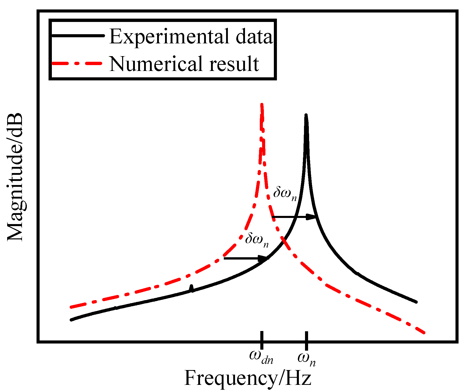
The FRFs of the real experimental model and the FE model around the nth natural frequency is shown in Figure 1. The modeling errors will cause the FRFs of the same mode order to move along the coordinate axis to a certain extent, but the basic shape does not change significantly.

The approximate estimation of the FRFs H_d(ω) near the resonance region can be expressed as

$${\mathit{H}}_d\left(\omega \right)\cong \mathit{H}\left(\omega +\delta {\omega }_n\right),n=1,\cdots ,m$$

(28)

where

$$\delta {\omega }_n={\omega }_n-{\omega }_{dn},n=1,\cdots ,m$$

(29)

where, ω_n and ω_dn are the nth natural frequency of the real experimental model and the FE model, respectively, δω_n is the frequency variation of the real experimental model and the FE model, and m is the order of the natural frequency taken by simulation.

The frequency range of model updating is expressed as ‘$\overline{\omega }$’. According to Equations (28) and (29), H_d(ω) on ‘$\overline{\omega }$’ can be approximately expressed as

$${\mathit{H}}_d\left(\overline{\omega }\right)\cong {\displaystyle \underset{n=1}{\overset{m}{\cup }}\mathit{H}\left(\overline{\omega }+\delta {\omega }_n\right)}={{\displaystyle \underset{n=1}{\overset{m}{\cup }}\left(-{\left(\overline{\omega }+\delta {\omega }_n\right)}^2\left(\mathit{M}+\delta \mathit{M}\right)+j\left(\overline{\omega }+\delta {\omega }_n\right)\left(\mathit{C}+\delta \mathit{C}\right)+\mathit{K}+\delta \mathit{K}\right)}}^{-1}$$

(30)

After repeated iterative calculations, the structural parameters of the FE model will be constantly updated and gradually approach to the parameters of the real experimental model. Therefore, in Equations (28) and (29), the initial frequency ω_n and FRFs H(ω) will be constantly updated iteratively and converge to the natural frequency and FRFs of the real experimental model.

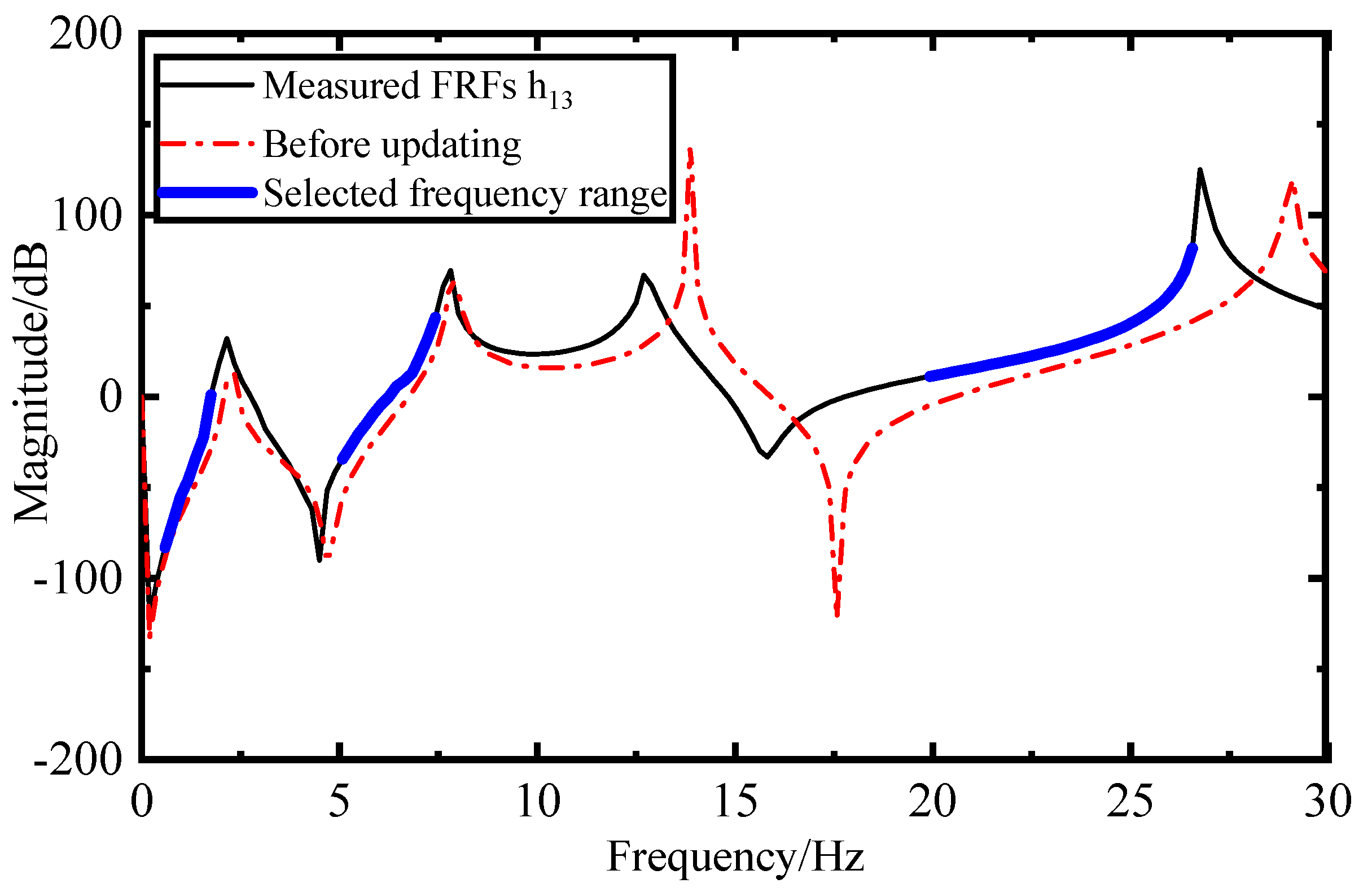
At present, most of the damping models cannot accurately simulate the actual damping effect but will increase the model errors and affect the result of model updating. Therefore, the damping parameter is not updated in this paper, so the influence of structural damping on the result of model updating should be reduced. From the analysis in Section 2.2, the damping has little effect on the frequency response amplitude when far away from the resonance peak. Therefore, the selection of appropriate frequency range can alleviate the influence of damping on the results of model updating, and the influence of damping can be ignored when the model is updated based on FRFs. The frequency close to resonance would be affected by damping, so the small region of about 4Hz around resonance was not considered in the model updating process [14].

If the two adjacent resonant peaks are too close to each other, the variation of FRFs in the frequency band between them cannot be guaranteed to decrease monotonically in the updating process, so this region is excluded to avoid the amplitude nonlinear problem. In each iteration, the frequency range also needs to be adjusted according to the change of the resonance point.

3. Implementation Procedure

Figure 2 is a flowchart of the model updating method using FRFs based on Sherman–Morrison formula, with the steps described below:

• Establish the FE analysis model, and extract the mass matrix M₁ and the stiffness matrix K₁ of the original model to obtain the dynamic stiffness matrix Z(ω) of the system, and calculate the FRFs, that is H(ω);
• Select several parameters that have an impact on the dynamic characteristics of the structure as the initial variables P₁, and P₁ become P₂ by perturbations, and the variation is ΔP; extract the mass matrix M₂ and the stiffness matrix K₂ of the changed model to obtain the variation of dynamic stiffness matrix of the system, that is ΔZ(ω), and recalculate the FRFs H*(ω) after parameter perturbations by using Sherman–Morrison formula;
• Select the appropriate frequency range which is away from the resonance for model updating and obtain the sensitivity S of the FRFs to the designed parameters.
• Conduct the model updating by the obtained sensitivity S, and the FRFs was iteratively updated by using Equation (27), obtain the variation P_n+1 − P_n, if the variables P_n are converged, stop; otherwise set n = n + 1, go to step (2); the stop criterion is $\Vert {\mathit{P}}_{n+1}-{\mathit{P}}_{nn}\Vert \le {10}^{-6}$;

4. Case Study

The simulation examples of the truss and the solar wing and the experiment of aluminum solar panel frame are used to verify the feasibility of the model updating method using FRFs based on Sherman–Morrison formula in this section.

4.1. Truss Structure

In this section, the FE model of truss structure is used for model updating, and considering the results under the interference of noise at the same time, so as to verify the feasibility of the model updating method using FRFs based on Sherman–Morrison formula.

4.1.1. Finite Element (FE) Modeling

The truss structure model is shown in Figure 3, numerically modeled by the ‘Matlab’ programming software. To simply to verify the feasibility of the method, each beam is discretized into a beam element, there are 21 discrete beam elements and 12 nodes, each node contains translational degrees of freedom (DOFs) in X direction and Y direction. Due to the Node 1 is fixed and Node 12 is fixed on the hinge support, so the translational DOFs x₁ and y₁ in X direction and Y direction of Node 1 and translational DOFs y₁₂ in Y direction of Node 12 are locked, so the total DOFs of the truss structure is 21. It is assumed that the DOFs of the target model that need to be updated and the FE model are matched, so there is no problem of model reduction and modal expansion. Therefore, the degrees of freedom of both the FE model and the target model is 21. The elastic modulus of all beam elements in the initial FE analysis is E = 70 Gpa, the density of the truss-element material is ρ = 2700 kg/m³, the length of each beam is L = 1 m, and the cross-sectional area of each truss element is A = 1 × 10⁻⁴ m².

It is assumed that the FE model of the truss structure has modeling errors, and the elastic modulus of beam element 1, 6, 11, 14, and 21 of the target model is 1.1, 1.2, 1.2, 1.2, and 1.1 times of the FE model, which is bold in red in Figure 3. It is assumed that the simulation experiment is a single point excitation, and the excitation point and response point in the target model is the same one. Using the above data for FE analysis, the frequencies of the first 7 order and FRFs of Node 4 and Node 10 are selected as the target value for model updating. Because the planar truss system is modeled in undamped mode, the influence of damping on FRFs at resonance peak need not be considered in the updating progress.

4.1.2. Comparison of Sensitivity Analysis

To further more intuitively illustrate the accuracy and efficiency of the proposed method in sensitivity calculating, we make 10⁻¹, 10⁻², and 10⁻³ of the perturbations in the elastic modulus respectively and compare the proposed method with the analytic derivatives method of Equation (4) to obtain the results shown in Figure 4.

The following error index O is used to quantify the accuracy of the sensitivity of the FRFs:

$$\mathit{O}=\frac{{\displaystyle \sum {}_{i=1}^N\left(\left|{\mathit{S}}_i^{Exact}-{\mathit{S}}_i^{Proposed}\right|/{\mathit{S}}_i^{Exact}\right)}}{N}\times \mathrm{100\%}$$

(31)

where N is the number of points on the curves. S_i^Exact and S_i^Proposed are the sensitivities of the FRFs obtained by analytical derivatives method of Equation (4) and the proposed method, respectively. A smaller O indicates a more accurate result.

The results in Figure 4 show that under different perturbations, the sensitivity calculated by the proposed method compares reasonably well with that calculated by the analytical derivatives. The small figure in the blue dashed box in Figure 4 is a local magnification comparison of the sensitivity curves calculated by the proposed method and the analytical derivatives method under different perturbations. With the decrease of the perturbation value, the sensitivity calculated by the proposed method is closer to that of the analytic derivatives method.

As shown in

Table 1. Errors between Proposed Method and Analytical Derivatives.

Perturbation	Error/%
10−3	0.01
10−2	0.24
10−1	1.78

, the error is only 0.01% for the perturbation of 10⁻³, which shows that the proposed method can carry out sensitivity analysis sufficient accurately for small variations in the design parameters. It can also be found that although the sensitivity calculated by the two different methods is basically the same, the calculation efficiency of the proposed method in this paper is higher than that of the analytic derivatives method as is shown in

Table 2. Comparison of the Time Cost.

	The Analytic Derivatives Method	The Proposed Method
Time Cost/s	0.842	0.653

. This advantage will be of great use for model updating of large-scale engineering structures, which can save much computation time.

4.1.3. Parameter Updating

Due to the inevitable interference of various noises in the real experiment, in order to simulate the real experiment state and test the anti-noise interference ability of the method proposed in this paper, 5% random white noise was added to the target value which was obtained in Section 4.1.1 in the form of H**(ω) = H*(ω) (1 + 0.05 μ), where the μ is a random number of −1~1, H*(ω) is the target value obtained in Section 4.1.1, and H**(ω) is the FRFs after adding random white noise. Then, the parameter updating formula shown in Equation (27) was used for 15 iterative computations. The frequency comparison between the FE model and the target model before and after modal updating is shown in

Table 3. Comparison of Frequency Values between FE Model and Target Model Under 5% White Noise.

Mode No.	Target Value/Hz	Before Updating/Hz	Errorb/%	After Updating/Hz	Errora/%
1	76.58	75.68	−1.18	76.20	−0.50
2	140.88	140.11	−0.55	141.25	0.26
3	214.29	211.18	−1.45	214.13	−0.07
4	301.78	296.74	−1.67	300.44	−0.44
5	361.41	353.91	−2.08	359.87	−0.43
6	430.42	422.08	−1.94	429.76	−0.15
7	460.18	445.16	−3.26	462.16	0.43

, and the comparison results of the updated parameters are shown in

Table 4. Comparison of Parameters Before and After Model Updating Under 5% White Noise.

Element ID	Target Value/Gpa	Before Updating/Gpa	Errorb/%	After Updating/Gpa	Errora/%
1	77.00	70.00	10.00	77.66	0.85
6	84.00	70.00	20.00	84.62	0.74
11	84.00	70.00	20.00	83.61	−0.47
14	84.00	70.00	20.00	83.29	−0.85
21	77.00	70.00	10.00	76.64	−0.47

. The convergence process of updated parameters is shown in Figure 5. The comparison of FRFs before and after updating is shown in Figure 6 and Figure 7.

The model updating process uses the frequencies of the first 5 order of the target value and their corresponding FRFs, while the fifth and sixth frequencies and their corresponding FRFs do not directly participate in the updating, but are used to evaluate the accuracy of the model updating method which is proposed in this paper.

Where Error_b and Error_a is the relative error between the frequency values of the FE model before and after the updating and the target value, respectively.

As can be seen from Table 3, under the excitation of 5% random white noise, there is a significant difference between the frequency of the FE model and the target model before the modal updating, and the maximum frequency error has reached −3.26%. This indicates that the reliability of the FE model is questionable, so it is necessary to update the initial FE model to improve the accuracy and reliability. After using the Sherman–Morrison formula proposed in this paper, the maximum error of the frequency of the first 7 order after modal updating is only −0.50%, which verifies that the model updating method using FRFs based on Sherman–Morrison formula has a good anti-noise performance.

Where Error_b and Error_a is the relative error between the elastic modulus of the FE model before and after the updating and the target value, respectively.

The model updating results of elastic modulus are shown in Table 4, under the excitation of 5% random white noise, the maximum relative error of the corrected elastic modulus is changed from 20.00% to −0.85%. Compared with the result in noiseless environment, the maximum error of the elastic modulus is within 1%, which greatly improves the reliability of the FE model and verifies the feasibility of the model updating method in this paper.

It can also be seen from the iterative convergence diagram of elastic modulus E of the truss in Figure 5, under the excitation of 5% random white noise, after 15 iterative computations, each parameter tends to converge, and the maximum error of each parameter is within ±1.00% after convergence. Therefore, the results verify that the model updating method using FRFs based on Sherman–Morrison formula is still applicable in noisy environment.

As shown in Figure 6 and Figure 7, the FRFs before and after updating are compared with the target value under 5% random white noise. There is obviously a big gap between the FRFs of the FE model before updating and the target model under 5% random white noise, and the FRFs data of the FE model almost completely coincides with the target value after updating, which shows that the model updating method using FRFs based on Sherman–Morrison formula can effectively reduce noise interference.

Each iteration is based on the sensitivity of the response at all the frequency points involved in the model updating. However, too many frequency points involved in the updating will greatly increase the computation and affect the efficiency of model updating. The change of FRFs is often discontinuous at the resonance peak, which especially happens in the low-damping structure. Therefore, the iterative process will not converge when the response of the frequency points close to the resonance peak are used for updating. So, it is generally necessary to select the frequency point carefully before model updating.

Taking the FRFs of Node 10 under 5% random white noise as an example, three frequency points selection cases are presented are given as follows, and the influence of them on the results of model updating is compared by observing the convergence of the elastic modulus of each element.

• Case 1: Select one frequency point every 10 Hz in the frequency band from 0 to 400 Hz and select 40 points in total.
• Case 2: Select 40 points randomly in the frequency band from 0 to 400 Hz.
• Case 3: Select 8 frequency points at the interval of 0.5 Hz from 10 Hz to the left of each resonance peak in the frequency band from 0 to 400 Hz and select 40 points in total.

Figure 8 shows the comparison of elastic modulus updating results of three cases. Since the frequency points selected by Case 1 and Case 2 do not avoid the resonance peak, so the FRFs are discontinuous which causes the elastic modulus of the two cases is not convergent. While only after 7 iterations, the elastic modulus of Case 3 is convergent. However, due to the noise pollution of 5% in the FRFs data, the result does not converge to 0%, but the maximum error is within ±1.5%.

By comparing the results of model updating using all the FRFs data, it can be seen that only a small amount of FRFs data is needed to complete the model updating, which indicates that the correct selection of frequency points can effectively improve the computational efficiency of model updating, and further proves that the proposed method has high computational efficiency and accuracy. Furthermore, only a small amount of FRFs data can be selected to complete the model updating quickly, the result is not very perfect compared with the result of using all frequency points, which indicates that increasing the frequency point can correspondingly increase the information contained in the FRFs data, which is an effective means to improve the quality of model updating.

4.2. Solar Wing

In this section, the FE model of solar wing is used for model updating to verify the feasibility of the model updating method using FRFs based on Sherman–Morrison formula.

4.2.1. FE Modeling

A complete FE model of the solar wing was modeled by the FE analysis software ‘Nastran’ based on the size diagram of the solar wing model as shown in Figure 9. The solar wing is an up-down axisymmetric structure, consisting of two plates with identical materials and geometric shapes. Each plate is divided into 12 shell elements numbered 1~24, and the two plates are connected by beam elements numbered 25~34. The solar wing model consists of 34 elements and 47 nodes, each node contains translational and rotational DOFs in the direction of X, Y, and Z. Since Node 44, 45, and 46 are fixed, and the rest are hinged, the translational and rotational DOFs in the X, Y, and Z directions of these three nodes are all locked. Therefore, the total DOFs of the solar wing structure is 264. The material parameters of the finite element model are as follows: the elastic modulus of the beam is E₁ = 200 Gpa, the density is ρ₁ = 7850 kg/m³, the cross-sectional area of the beam is A₁ = 4 × 10⁻⁴ m², and the poisson ratio is μ₁ = 0.32. The elastic modulus of the solar wing is E₂ = 70 Gpa, the density is ρ₂ = 2700 kg/m³, the thickness is t = 4 × 10⁻³ m, and the poisson ratio is μ₂ = 0.34. To simulate the actual damping of the model, the Rayleigh proportional damping model is adopted, as is shown below

$$\mathit{C}=a\mathit{M}+b\mathit{K}$$

(32)

where C represents the damping matrix of the system, M represents the mass matrix of the system, K represents the stiffness matrix of the system, a and b represent the damping coefficients. In this case, the actual damping coefficients are assumed to be a = 0.2 and b = 0.0005.

The comparison of frequency values between the FE model and the target model under 5% white noise is shown in

Table 5. Comparison of Frequency Values between FE Model and Target model Under 5% White noise.

Mode No.	Target Value/Hz	Before Updating/Hz	Errorb/%	After Updating/Hz	Errora/%
1	0.25	0.24	−4.00	0.25	0
2	0.91	0.86	−5.49	0.90	−1.10
3	2.09	1.99	−4.78	2.08	−0.48
4	4.44	4.24	−4.50	4.38	−1.35
5	5.69	5.43	−4.57	5.68	−0.18
6	8.63	8.23	−4.63	8.59	−0.46
7	9.35	8.93	−4.49	9.29	−0.64

. The modeling errors of the target model that needs to be updated and the FE model are shown in

Table 6. Comparison of Parameters Before and After Model Updating Under 5% White noise.

Parameters	Target Value	Before Updating	Errorb/%	After Updating	Errora/%
E1/Gpa	273.00	210.00	30.00	272.35	−0.24
E2/Gpa	84.00	70.00	20.00	84.23	0.27
ρ1/kg/m3	9027.50	7850.00	15.00	9002.22	−0.28
A1/m2	4.80 × 10−4	4.00 × 10−4	20.00	4.82 × 10−4	0.42

. There are initial errors of 30.00%, 20.00%, 15.00%, and 20.00% in E₁, E₂, ρ₁, and A₁, respectively. It is assumed that the simulation experiment is a single point excitation, and the excitation point and response point in the target model is the same one. The frequency of the first 7 order and FRFs of Node 13 and Node 26 are obtained as the target value to conduct the model updating progress.

4.2.2. Parameter Updating

The elastic modulus of the connecting beams and the solar wing, and the density and the cross-sectional area of the connecting beams are updated in turn with the strategy of step by step. Meanwhile, 5% random white noise was added to the target value of the FRF data obtained in Section 4.2.1 to simulate the real experimental situation in the form of H**(ω) = H*(ω) (1 + 0.05μ), where the μ is a random number of −1~1, H*(ω) is the target value obtained in Section 4.2.1, and H**(ω) is the FRFs after adding random white noise. Then, the parameter updating formula shown in Equation (27) was used for 20 iterative computations.

The model updating process uses the frequencies of the first 5 order of the target model and their corresponding FRFs, while the fifth and sixth frequencies and their corresponding FRFs do not directly participate in the updating, but are used to evaluate the accuracy of the model updating method which is proposed in this paper. Combined with the rules in Section 2.3, the frequency of the model updating is selected as the frequency point near the resonance region that is shown in Figure 10. Remove the low frequency band containing the first two resonance regions, and to avoid the problem of amplitude nonlinearity, the frequency points between the fourth and fifth resonances are ignored.

Where Error_b and Error_a is the relative error between the frequency values of the FE model before and after the updating and the target value, respectively.

As can be seen from Table 5, under the excitation of 10% random white noise, the maximum relative error of the frequency is changed from −5.49% to −1.10%, which verifies the effectiveness and anti-noise performance of the proposed method in this paper.

Where Error_b and Error_a is the relative error between the parameters of the FE model before and after the updating and the target value, respectively.

The model updating results of parameters are shown in Table 6, under the excitation of 10% random white noise, the maximum relative error of the updated parameters is changed from 30.00% to −0.24%, which greatly improves the reliability of the FE model and verifies the feasibility of the model updating method in this paper.

As shown in Figure 11 and Figure 12, due to modeling errors between the target model and the FE model, there is obviously a big gap between the FRFs of the FE model before updating and the target model under 5% random white noise. While after 20 iterative computations, the error between the obtained FRFs and the target value is quite close, which shows that the model updating method using FRFs based on Sherman–Morrison formula can effectively reduce noise interference. At the same time, the influence of damping on the amplitude of FRFs is effectively reduced by choosing the appropriate frequency range. Therefore, the results verify that the model updating method using FRFs based on Sherman–Morrison formula has a good anti-noise performance.

4.3. Experimental Verification

4.3.1. Modal Test

To investigate the applicability of the proposed method in practical engineering, a simplified aluminum solar panel frame is designed at the dimensions shown in Figure 13. This only considers the frame components and ignores the influence of supporting structure and hinge. The connection between plate and plate is directly integrated.

The piezoelectric accelerometers were adopted in this modal test, which with a mass of 20 g, charge sensitivity of 6.05 pC/ms², and frequency range from 0.5 Hz to 5 kHz. The CL-YD-303 hammer was also adopted, the reference sensitivity is 3.99 pC/N. CRAS V7.0, a vibration and dynamic signal acquisition and analysis system developed by Nanjing AnZheng Software Engineering Company, was used as the analytical instrument, and MaCras was used as the modal analysis software.

The layout of test site is shown in Figure 14a. The end of the solar panel frame is fixed with a support, and the two accelerometers are installed on Position 1 and Position 2, where the mass of Accelerometer 1 is m₁ = 20 g and the mass of Accelerometer 2 is m₂ = 20 g. Then make a single point excitation at Position 3 with the hammer to measure the FRFs within 0~30 Hz of the solar panel frame. The FRFs obtained after 5 excitations are fitted by MaCras.

The FE model of the solar panel frame was modeled by the FE analysis software ‘Nastran’ as shown in Figure 14b, which consists of 86 shell elements and 148 nodes. The mass points were established at Node 1 and Node 2 to conduct the model updating and both the mass identification of the two accelerometers through mass perturbation of the mass points.

4.3.2. Parameter Updating

Take the FRFs h₁₃ measured by Accelerometer 1 as an example. Combined with the rules in Section 2.3, the frequency of the model updating is selected as the frequency point near the resonance region, and to avoid the problem of amplitude nonlinearity, the frequency points of the third resonances are ignored as is shown in Figure 15.

Where Error_b and Error_a is the relative error between the frequency values of the FE model before and after the updating and the experimental value, respectively.

As can be seen from

Table 7. Comparison of Frequency Values between FE Model and Experimental Model.

Mode No.	Experimental/Hz	Before Updating/Hz	Errorb/%	After Updating/Hz	Errora/%
1	2.15	2.34	8.84	2.15	0
2	7.81	7.92	1.41	7.62	−2.43
3	12.71	13.87	9.13	13.09	2.99
4	26.76	29.10	8.74	27.15	1.46

, after several iterative computations, the maximum relative error of the frequency is changed from 9.13% to 2.99%. Although the error between the second order frequency and the experimental value increased slightly after updating, the average error of the first four orders decreased from 7.03% to 1.72%, which verifies the effectiveness of the proposed method in this paper.

The identification results of accelerometer mass are shown in

Table 8. The Identification Results of Accelerometer Mass.

Parameters	Experimental	Identification
m1/g	20.00	17.78
m2/g	20.00	17.32

. Since the accelerometer is attached with wires, the identification results will be affected to some extent, so it can be considered that the identification results are within the ideal range, which greatly improves the reliability of the FE model and verifies the feasibility of the model updating method proposed in this paper.

As shown in Figure 16, due to the additional mass of the accelerometers between the real experimental model and the FE model, there is obviously a big gap between the FRFs of the FE model before updating and the experimental structure. While after several iterative computations, the error between the obtained FRFs and the real experimental value h₁₃ is quite close, which shows that the proposed method has a good model updating capability and engineering application.

At the same time, the experimental modal shapes are measured to compare with the FE modal shapes, to further verify the accuracy of the proposed method. Due to the limitation of test conditions, it is difficult to measure the displacement of all nodes. Therefore, 24 points as shown in Figure 17a are selected to measure the displacement in the Z direction by the hammer. The first 4 modal shapes of the experiment model are obtained by MaCras. Meanwhile, 24 nodes of the FE model corresponding to the measured points of the experimental model are selected, as shown in Figure 17b. The first 4 modal shapes of the FE model before and after updating are obtained through FE analysis.

Using modal assurance criteria (MAC) to verify the mutual independence and consistency of the modal shapes between the first 4 order of the FE model before and after updating and the corresponding experimental model:

$$MAC=\frac{{\left|{\varphi }_u{}^T{\varphi }_v\right|}^2}{{\varphi }_u{}^T{\varphi }_u{\varphi }_v{}^T{\varphi }_v}$$

(33)

The ϕ_u, ϕ_v are the modal vector of the FE model and the experimental model, respectively, which are all the column vector, u, v is the modal order.

Theoretically, if the two models are the same physical modal, the MAC value is 1, if the two models are not the same physical modal or if the modal vectors are independent of each other, the MAC value is 0. The MAC value will be affected due to the nonlinearity of the structure, external noise interference of the measured data and improper data processing. It is generally believed that if MAC value is greater than 0.9, the two models are related, and if MAC value is less than 0.05, the two models are unrelated.

Table 9. Comparison of Modal Shapes Before and After Model Updating.

Mode No.	Experimental	Before Updating	After Updating
1
2
3
4

shows the comparison of modal shapes between the first 4 order of the FE model before and after updating and the corresponding experimental model. The first modal of the solar panel frame is first-order bending around X axis; the second modal is first-order torsion around Y axis; the third modal is second-order bending around X axis; the fourth modal is second-order torsion around Y axis. The blue line in the modal shape diagram represents the fixed side.

It can be seen from Figure 18 that, after several iterative computations, the MAC value of the first 4 orders after updating are all improved, indicating that the FE modal shapes after updating are well matching with the experimental ones, which further verifies the accuracy requirement of the proposed method.

5. Conclusions

A model updating method using FRFs based on Sherman–Morrison sensitivity is proposed in this paper. The sensitivity of FRFs is calculated using Sherman–Morrison formula which avoids recalculation of FE dynamic analysis. The simulation examples of truss and solar wing and the experiment of aluminum solar panel frame are implemented to verify the accuracy of the proposed method. The following conclusions can be drawn:

• Only the initial FRFs and parameter perturbations are employed for the acquisition of sensitivity, which avoids recalculation of FE dynamic analysis, and improves the efficiency of analysis and calculation at the same time. Only a small amount of FRFs data is needed to complete the model updating process.
• With the effect of 5% random white noise, the parameter error after updating is within ±1.00%, which shows that the proposed method has a certain anti-noise capability. The experiment study shows that the proposed method can effectively identify the structural parameters.
• Selecting appropriate frequency range and points can effectively improve the stability and efficiency of model updating. In addition, the method can consider multiple parameters simultaneously and has great potential for engineering application.

References

1. Mottershead, J.E.; Link, M.; Friswell, M.I. The sensitivity method in finite element model updating: A tutorial. Mech. Syst. Signal Proc. 2011, 25, 2275–2296. [Google Scholar] [CrossRef]
2. Wang, Z.; Xin, Y.; Ren, W.X. Nonlinear structural joint model updating based on instantaneous characteristics of dynamic responses. Mech. Syst. Signal Proc. 2016, 76–77, 476–496. [Google Scholar] [CrossRef]
3. Feng, X.; Jing, X.; Xu, Z.; Guo, Y. Bio-inspired anti-vibration with nonlinear inertia coupling. Mech. Syst. Signal Proc. 2019, 124, 562–595. [Google Scholar] [CrossRef]
4. Wan, Z.; Wang, T.; Huang, Q.; Wang, J. Acoustic finite element model updating using acoustic frequency response function. Finite Elem. Anal. Des. 2014, 87, 1–9. [Google Scholar] [CrossRef]
5. Rosenzveig, G.; Louf, F.; Champaney, L. A FE model updating method for the simulation of the assembly process of large and lightweight aeronautical structures. Finite Elem. Anal. Des. 2016, 111, 56–63. [Google Scholar] [CrossRef] [Green Version]
6. Guo, Y.; Xu, Z.; Chen, B.; Ran, C.; Guo, W. Preparation and Experimental Study of Magnetorheological Fluids for Vibration Control. Int. J. Acoust. Vib. 2017, 22, 194–200. [Google Scholar] [CrossRef]
7. Sehgal, S.; Kumar, H. Structural Dynamic Model Updating Techniques: A State of the Art Review. Arch. Comput. Method Eng. 2015, 23, 515–533. [Google Scholar] [CrossRef]
8. Chakraborty, S.; Sen, A. Adaptive response surface based efficient Finite Element Model Updating. Finite Elem. Anal. Des. 2014, 80, 33–40. [Google Scholar] [CrossRef]
9. Shabbir, F.; Omenzetter, P. Particle Swarm Optimization with Sequential Niche Technique for Dynamic Finite Element Model Updating. Comput.-Aided Civ. Infrastruct. Eng. 2015, 30, 359–375. [Google Scholar] [CrossRef] [Green Version]
10. Behmanesh, I.; Moaveni, B.; Lombaert, G.; Papadimitriou, C. Hierarchical Bayesian model updating for structural identification. Mech. Syst. Signal Proc. 2015, 64–65, 360–376. [Google Scholar] [CrossRef] [Green Version]
11. Zhan, M.; Guo, Q.T.; Yue, L.; Zhang, B.Q. Finite Element Model Updating Using Strain Mode and Genetic Algorithm-Based Method. J. Vib. Meas. Diag. 2018, 38, 974–978. [Google Scholar]
12. Wang, Z.C.; Xin, Y.; Ren, W.X. Nonlinear structural model updating based on instantaneous frequencies and amplitudes of the decomposed dynamic responses. Eng. Struct. 2015, 100, 189–200. [Google Scholar] [CrossRef]
13. Zang, C.; Schwingshackl, C.W.; Ewins, D.J. Model validation for structural dynamic analysis: An approach to the Sandia structural dynamics challenge. Comput. Meth. Appl. Mech. Eng. 2008, 197, 2645–2659. [Google Scholar] [CrossRef]
14. Shadan, F.; Khoshnoudian, F.; Esfandiari, A. A frequency response-based structural damage identification using model updating method. Struct. Control. Health Monit. 2016, 23, 286–302. [Google Scholar] [CrossRef]
15. Shadan, F.; Khoshnoudian, F.; Inman, D.J.; Esfandiari, A. Experimental validation of a FRF-based model updating method. J. Vib. Control. 2016, 24, 1570–1583. [Google Scholar] [CrossRef]
16. Esfandiari, A.; Bakhtiari-Nejad, F.; Rahai, A.; Sanayei, M. Structural model updating using frequency response function and quasi-linear sensitivity equation. J. Sound Vibr. 2009, 326, 557–573. [Google Scholar] [CrossRef]
17. Esfandiari, A.; Bakhtiari-Nejad, F.; Sanayei, M.; Rahai, A. Structural finite element model updating using transfer function data. Comput. Struct. 2009, 88, 54–64. [Google Scholar] [CrossRef]
18. Pradhan, S.; Modak, S.V. Damping Matrix Identification by Finite Element Model Updating Using Frequency Response Data. Int. J. Struct. Stab. Dyn. 2017, 17, 1–27. [Google Scholar] [CrossRef]
19. Li, W.M.; Hong, J.Z. Research on the iterative method for model updating based on the frequency response function. Acta Mech. Sin. 2012, 28, 450–457. [Google Scholar] [CrossRef]
20. Hong, Y.; Pu, Q.H.; Wang, Y.; Chen, L.J.; Gou, H.Y.; Li, X.B. Model-updating with experimental frequency response function considering general damping. Adv. Struct. Eng. 2017, 21, 82–92. [Google Scholar] [CrossRef] [Green Version]
21. Wang, X.; Hill, T.L.; Neild, S.A.; Shaw, A.D.; Haddad Khodaparast, H.; Friswell, M.I. Model updating strategy for structures with localised nonlinearities using frequency response measurements. Mech. Syst. Signal Proc. 2018, 100, 940–961. [Google Scholar] [CrossRef] [Green Version]
22. Wang, X.; Hill, T.L.; Neild, S.A. Frequency response expansion strategy for nonlinear structures. Mech. Syst. Signal Proc. 2019, 116, 505–529. [Google Scholar] [CrossRef] [Green Version]
23. Weng, S.; Zhu, H.P.; Xia, Y.; Ye, L.; Hu, X.Y. Construction of Stiffness and Flexibility for Substructure-Based Model Updating. Math. Probl. Eng. 2013, 2013, 706798. [Google Scholar] [CrossRef] [Green Version]
24. Sipple, J.D.; Sanayei, M. Finite element model updating using frequency response functions and numerical sensitivities. Struct. Control. Health Monit. 2013, 21, 784–802. [Google Scholar] [CrossRef]
25. Weng, S.; Xia, Y.; Xu, Y.L.; Zhu, H.P. An iterative substructuring approach to the calculation of eigensolution and eigensensitivity. J. Sound Vib. 2011, 330, 3368–3380. [Google Scholar] [CrossRef]
26. Jiang, D.; Xu, Y.; Zhu, D.; Cao, Z. Temperature-dependent thermo-elastic parameter identification for composites using thermal modal data. Adv. Mech. Eng. 2019, 11, 1687814019884165. [Google Scholar] [CrossRef] [Green Version]
27. Rezaiee-Pajand, M.; Entezami, A.; Sarmadi, H. A sensitivity-based finite element model updating based on unconstrained optimization problem and regularized solution methods. Struct. Control. Health Monit. 2020, 27, e2481. [Google Scholar] [CrossRef]
28. Esfandiari, A.; Sanayei, M.; Bakhtiari-Nejad, F.; Rahai, A. Finite Element Model Updating Using Frequency Response Function of Incomplete Strain Data. AIAA J. 2010, 48, 1420–1433. [Google Scholar] [CrossRef]
29. Dopico, D.; Zhu, Y.T.; Sandu, A.; Sandu, C. Direct and Adjoint Sensitivity Analysis of Ordinary Differential Equation Multibody Formulations. J. Comput. Nonlinear Dyn. 2015, 10, 111–118. [Google Scholar] [CrossRef]
30. Zuo, W.J.; Bai, J.T.; Yu, J.F. Sensitivity reanalysis of static displacement using Taylor series expansion and combined approximate method. Struct. Multidiscip. Optim. 2016, 53, 953–959. [Google Scholar] [CrossRef]
31. Turan, A.; Mugan, A. Structural and sensitivity reanalyses based on singular value decomposition. Struct. Multidiscip. Optim. 2013, 48, 327–337. [Google Scholar] [CrossRef]
32. Zhu, R.; Fei, Q.G.; Jiang, D.; Cao, Z.F. Dynamic Sensitivity Analysis Based on Sherman-Morrison-Woodbury Formula. AIAA J. 2019, 57, 4992–5001. [Google Scholar] [CrossRef]
33. Zhu, R.; Fei, Q.G.; Jiang, D.; Cao, Z.F. Removing mass loading effects of multi-transducers using Sherman-Morrison-Woodbury formula in modal test. Aerosp. Sci. Technol. 2019, 93, 105241. [Google Scholar] [CrossRef]
34. Zhu, R.; Fei, Q.G.; Jiang, D.; Cao, Z.F. Maintaining Specific Natural Frequency of Damped System despite Mass Modification. Int. J. Aerosp. Eng. 2019, 2019, 1947506. [Google Scholar] [CrossRef]
35. Zhu, R.; Fei, Q.G.; Jiang, D.; Hang, X.C. Using Sherman-Morrison theory to remove the coupled effects of multi-transducers in vibration test. Proc. Inst. Mech. Eng. Part G-J. Aerosp. Eng. 2018, 233, 1364–1376. [Google Scholar] [CrossRef]
Figure 1. The frequency response function (FRF)’s of the real experimental model and the finite element (FE) model around the nth natural frequency.
Applsci 10 04985 g001
Figure 2. Model updating implementation steps.
Applsci 10 04985 g002
Figure 3. Truss elements and nodes diagrams.
Applsci 10 04985 g003
Figure 4. Sensitivity of FRFs to elastic modulus.
Applsci 10 04985 g004
Figure 5. Convergence process of designed parameters under 5% white noise.
Applsci 10 04985 g005
Figure 6. Comparison of FRFs data measured at Node 4 under 5% random white noise.
Applsci 10 04985 g006
Figure 7. Comparison of FRFs data measured at Node 10 under 5% random white noise.
Applsci 10 04985 g007
Figure 8. Comparison of elastic modulus updating results of three cases: (a) Case 1; (b) Case 2; (c) Case 3.
Applsci 10 04985 g008
Figure 9. Dimensions of solar wing.
Applsci 10 04985 g009
Figure 10. Selected frequency range.
Applsci 10 04985 g010
Figure 11. Comparison of FRFs data measured at Node 13 under 5% random white noise.
Applsci 10 04985 g011
Figure 12. Comparison of FRFs data measured at Node 26 under 5% random white noise.
Applsci 10 04985 g012
Figure 13. Dimension of the aluminum solar panel frame.
Applsci 10 04985 g013
Figure 14. Accelerometers and excitation point: (a) Experimental arrangement; (b) FE model.
Applsci 10 04985 g014
Figure 15. Selected frequency range.
Applsci 10 04985 g015
Figure 16. Comparison of FRFs h13.
Applsci 10 04985 g016
Figure 17. Measurement of modal shapes: (a) Experimental model; (b) FE model.
Applsci 10 04985 g017
Figure 18. Comparison of MAC before and after model updating: (a) Before updating; (b) After updating.
Applsci 10 04985 g018