Deep Matrix Factorization Approach for Collaborative Filtering Recommender Systems

Abstract

Providing useful information to the users by recommending highly demanded products and services is a fundamental part of the business of many top tier companies. Recommender Systems make use of many sources of information to provide users with accurate predictions and novel recommendations of items. Here we propose, DeepMF, a novel collaborative filtering method that combines the Deep Learning paradigm with Matrix Factorization (MF) to improve the quality of both predictions and recommendations made to the user. Specifically, DeepMF performs successive refinements of a MF model with a layered architecture that uses the acquired knowledge in a layer as input for subsequent layers. Experimental results showed that the quality of both the predictions and recommendations of DeepMF overcome the baselines.

1. Introduction

Presently, data processing has become a priority for the society. The amount of information we generate every day is on the rise, mainly due to the increase in the number of devices we use routinely as well as new patterns of interaction with technology that have been developed over the last few years. With such a high volume of real-time data, Machine Learning (ml) techniques became a key tool for being able to extract knowledge from data. At present, ml is one of the most active research field not only within computer science, but also in healthcare [1], sociology [2] and industry [3].

One of the most important applications of ml are Recommender System (RS) [4], which are techniques that make use of different sources of information for providing users with predictions and recommendations of items, adjusting factors such as accuracy, novelty, sparsity and stability in the recommendations [5,6]. Top tier companies such as Netflix, Spotify and Amazon, use rs provide useful information to the users by recommending highly demanded products and services. Although it is possible to find many kinds of rs in the state of the art, they all share a key component: The filtering algorithm at the core. According to the filtering algorithm used, rs might be categorized [7] into (a) Collaborative Filtering (CF), (b) demographic filtering, (c) content-based filtering and (d) hybrid filtering. Regarding cf, Matrix Factorization (mf) is one of its most widely used techniques [4,8]. It operates by decomposing the user-item interaction matrix into the product of two lower dimensional rectangular matrices as well as assigning different regularization weights to the latent factors in order to improve the prediction results [9].

A major recent breakthrough in the field of ml is the so-called Deep Learning (dl) technology, that has attracted much attention not only from the scientific community, but also from society in general. Oppositely to other ml techniques, which can only extract knowledge from the shallow of the data, typically based on statistical evidence, dl is able to detect and exploit the underlying multi-layer structure of the data. Although dl is generally linked to artificial neural networks, the paradigm is more complex than that. As stated by LeCun et al. [10], “dl allows computational models that are composed of multiple processing layers to learn representations of data with multiple levels of abstraction”. Since its inception, dl has positioned as a very top notch technology for uncovering tangled structures in high-dimensional data. In this way, it has been applied to a wide range of domains such as speech recognition [11], image recognition [12] or natural language processing [13], among others.

As might be expected, rs have not been immune to the boom in dl and it is possible to find several works in this direction. The most obvious interplay is to apply deep neural networks [14] for improving the predictions of the RSs. Indeed, they provide appropriate a posteriori biases to the input data type, exploiting any inherent structure within the data. Furthermore, deep neural networks are capable of modeling the non-linearity in data with nonlinear activations, which is one of the principal aims of modern RS, making it possible to capture complex interaction patterns between users and items.

Due to the aforementioned advantages, neural networks with deep architectures, i.e., many layers, have been used to create new RS. For instance, DeepFM [15] is an approach that models the interactions of high and low order features through deep neural networks and factorization machines, respectively. On the other hand, Autoencoder-Based Collaborative Filtering (ACF) [16] uses another well-known dl architecture, namely variational autoencoders, to build a rs model that decompose the partial observed ratings vectors in a similar way as one-hot encoding. In the same way, Bobadilla et al. [17] provide an innovative dl architecture to improve cf results by exploiting the potential of the reliability concept to raise predictions and recommendations quality by incorporating prediction errors in the dl layers. Regarding convolutional neural networks, He et al. [18] propose to use them in order to enhance cf by using the outer product instead of the customary dot product to model the interaction patterns of both users and items, as well as capturing the high-order correlations among embedding dimensions. In addition, Abavisani and Patel [19] proposed an artificial neural network that consists of a convolutional autoencoder along with a fully connected layer to learn robust deep features for classification. Along the same lines, Recurrent Neural networks have been used with rs [20,21,22], although under some restrictions (i.e., session-based recommendations), due to the features of this kind of deep architecture, which are suitable for sequential data processing. Even Generative Adversarial Networks (GANs) have been used to generate negative samples for a memory network-based streaming rs [23] and enhancing the Bayesian personalized ranking with adversarial training [24].

Another promising line of application of dl is to pull apart the neural networks and to apply the underlying philosophy to extend the usual mf algorithm to get deep factorizations. This approach is a common trend in several machine learning contexts, but it has never been applied to RS. For instance, Le Magoarou and Gribonval proposed FAuST [25], a deep factorization method of a matrix into a product of many sparse factors that can be achieved through hierarchical refinements, in the spirit of deep networks. FAuST has proven to be very successful in image processing, data compression and inverse linear problems but, as we will see, it fails to provide a competitive alternative when applied to RS. In a similar vein, Trigeorgis et al. [26] devised a semi-supervised learning method based on Non-negative Matrix Factorization, which was applied to the problem of face clustering, while Guo and Zhang [27] used a similar approach to perform dimension reduction and pattern recognition. A multilevel decomposition method used to derive a feature representation for speech recognition is presented in [28], which outperforms existing features for various speech recognition tasks.

In this paper, we propose a novel method for incorporating dl to CF-based RSs. For that purpose, we present a new cf method that combines the dl paradigm with mf in order to improve the quality of predictions and recommendations. The approach presented here is based on the principles of dl, but unlike state-of-the-art works, the proposed method does not use deep neural network architectures. Instead, it transforms the mf process into a layered process, in which each layer factors out the errors made in the previous layer.

Roughly speaking, the proposed model works as follows. Consider a matrix R that collects the known ratings of the users of the rs to the supervised items. Typically, the mf looks for a factorization of the form $R\approx P·Q$ for some matrices $P,Q$ of low rank. In this way, the matrix $E^1=R-P·Q$ measures the error attained with the mf. The key point is that, if we were able to exactly predict the error, then we could correct the output of our model by tuning it to take into account the expected error. To get this, our proposal is to deepen this factorization and to look for a factorization of the error $E^1\approx P^1·Q^1$, which gives rise to a ‘second order error’ $E^2=E^1-P^1·Q^1$. This refinement of the expected error can be continued as many times as desired in order to achieve a better control of the error. In this way, as byproduct of the application of the dl process, we end up with a more accurate model that auto-corrects its predictions with the estimation of the expected error in the guess.

Summarizing, the proposed rs model follows the dl paradigm by performing successive refinements of a mf model with a layered architecture and letting it to use the acquired knowledge in one layer to be used as input for subsequent layers. The novelty of our work lies in using the concepts of dl, not for use with artificial neural networks, but to improve the mf itself.

The rest of the paper is structured as follows. Section 2 contains the material and methods used to formalize the proposed method, as well as the associated algorithm. Section 3 presents the results of the experimental evaluation conducted in order to measure the performance of the presented method. As we will see, the proposed algorithm consistently outperforms the previous mf methods that can be found in the literature. Finally, Section 4 discusses about these results and its impact on the rs research field.

2. Materials and Methods

A current trend in the field of cf is to improve the quality of the predictions by means of different techniques of mf, such as PMF [29], NMF [30], and SVD++ [31]. However, all these techniques rely on the same approach: they pose an optimization problem through a loss function that measures the divergence of the model of the expected behavior of users and items in a collaborative context from the actual behavior. Trying to break with this paradigm, in this paper we present a novel recommendation model that, using the mf paradigm, introduces the principles of dl to refine the output of the model through successive trainings. We named this new model Deep Matrix Factorization (DeepMF).

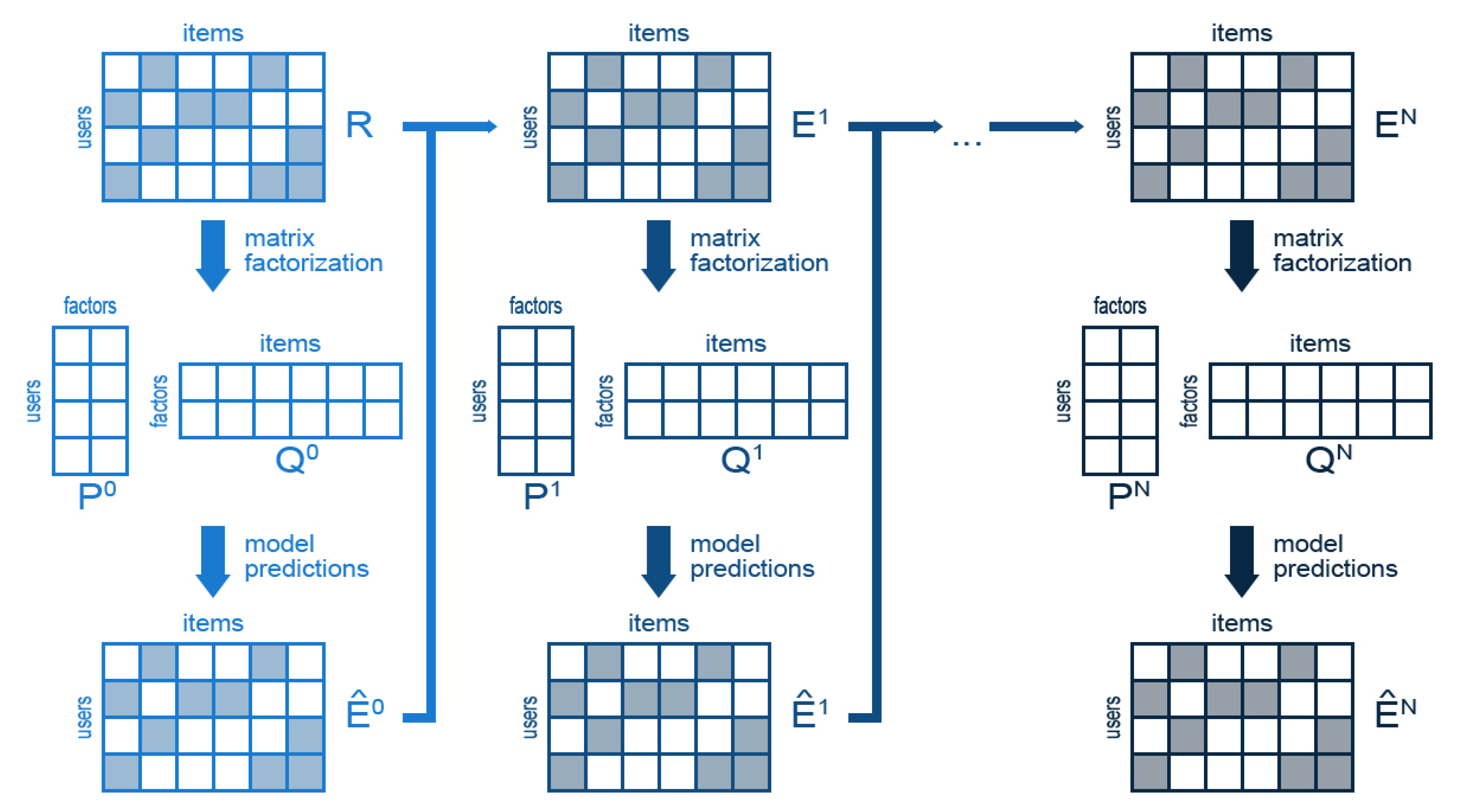
Figure 1 summarizes the operation of DeepMF. As we can observe, the model is initialized with the usual input of a CF-based RS: a matrix R that contains the ratings of the users to the items. Note that this matrix is sparse, since a user generally only votes a very small subset of the existing items. As in classical mf approaches, this matrix R, that will be also called $R=E^0$ in our context, is approximated by a dense matrix ${\widehat{E}}^0$ of the form ${\widehat{E}}^0=P^0·Q^0$, where $P^0$ and $Q^0$ are matrices of small rank. This matrix ${\widehat{E}}^0$ provides the predicted ratings at the first step.

At this point the dl begins. A new matrix $E^1=R-{\widehat{E}}^0$ is built by computing the attained errors between the original ratings R and the predicted ratings stored in ${\widehat{E}}^0$. This new matrix is, again, approximated by a factorization into two new small rank matrices ${\widehat{E}}^1=P^1·Q^1$, which produces the errors at the second step $E^2=E^1-{\widehat{E}}^1$. This process is repeated as many times as desired, by generating and factorizing successive error matrices $E^1,\dots ,E^N$. Presumably, this sequence of error matrices converges to zero, so we get preciser predictions as we add new layers to the model.

This method can be formalized as follows. Suppose that our cf-based rs is dealing with n users and m items, whose ratings are collected in a spare matrix $R=\left(R_{u,i}\right)\in {\mathbb{R}}^{n\times m}$, where $R_{u,i}$ is the rating that the user u gave to item i (typically, integer values between 1 and 5), or $R_{u,i}=•$ if u has not rated the item i. We look for a factorization of $E^0=R$ of the form $E^0\approx P^0·Q^0$, where $P^0$ is a $n\times k^0$ matrix and $Q^0$ is a $k^0\times m$ matrix. Here, $k^0$ is interpreted as the number of hidden factors we try to detect in the first step (typically $k^0$ is around 10) and $Q^0,P^0$ are seen as the projection/co-projection of the n users and m items into a $k^0$-dimensional latent space. These small rank matrices are learned such that the product $P^0·Q^0$ is a good approximation of the ratings matrix $E^0=R$, that is

$$E^0\approx {\widehat{E}}^0=P^0·Q^0$$

(1)

in the usual euclidean distance.

By subtracting the approximation performed by ${\widehat{E}}^0$ to the original matrix R we can obtain a new sparse matrix $E^1$ that contains the prediction error

$$E^1=R-{\widehat{E}}^0=E^0-P^0·Q^0.$$

(2)

Note that positive values in $E^1$ denotes that the prediction is too low and must be increased and negative values in $E_1$ denotes that the prediction is too high and must be decreased. As we stated before, the main contribution of the proposed method is its deep learning approach. This is achieved by performing a new factorization to the $E^1$ error matrix in such a way that

$$E^1\approx {\widehat{E}}^1=P^1·Q^1.$$

(3)

The matrices $P^1,Q^1$ have orders $n\times k^1$ and $k^1\times m$ for a certain number of latent factors $k^1$. Observe that we may take $k^1\ne k^0$ in order to get a different level of resolution in the factorization.

In the general case, if we computed $s-1$ steps of the deep learning procedure, we compute the s-th matrix of errors as

$$E^s=E^{s-1}-{\widehat{E}}^{s-1}=E^{s-1}-P^{s-1}·Q^{s-1},$$

(4)

and we look for a factorization into matrices $P^s$ of order $n\times k^s$ and $Q^s$ of order $k^s\times m$ such that, as much as possible in the euclidean norm,

$$E^s\approx {\widehat{E}}^s=P^s·Q^s.$$

(5)

Once the deep factorization process ends after N steps, the original rating matrix R can be reconstructed by adding the estimates of the errors as

$$\begin{array}{cc}\hfill R\approx \widehat{R}& ={\widehat{E}}^0+E^1={\widehat{E}}^0+{\widehat{E}}^1+E^2=\dots \approx {\widehat{E}}^0+{\widehat{E}}^1+{\widehat{E}}^2+\dots +{\widehat{E}}^N\hfill \\ \hfill & =P^0·Q^0+P^1·Q^1+\cdots +P^N·Q^N=\sum _{s=0}^N{P}^s·Q^s.\hfill \end{array}$$

(6)

For any step $s=0,\dots ,N$, the factorization $E^s\approx P^s·Q^s$ is sought by the standard method of minimizing the euclidean distance between $E^s$ and $P^s{Q}^s$ by gradient descent with regularization, as in PMF [29]. In this way, if we write $E^s=(e_{u,i}^s)$, the rows of $P^s$ are denoted by $p_1^s,p_2^s,\dots ,p_n^s$ and the columns of $Q^s$ are denoted by $q_1^s,q_2^s,\dots ,q_m^s$, the loss function is given by

$$\begin{array}{cc}\hfill {\mathcal{F}}^s(p_u^s,q_i^s)& =\left|\right|E^s-P^s·Q^s{\left|\right|}^2+{\lambda }^s\left(\sum _{u=1}^n\left|\right|p_u^s{\left|\right|}^2+\sum _{i=1}^m\left|\right|q_i^s{\left|\right|}^2\right)\hfill \\ \hfill & =\sum _{e_{u,i}^s\ne •}{\left(e_{u,i}^s-p_u^s·q_i^s\right)}^2+{\lambda }^s\left(\sum _{u=1}^n\left|\right|p_u^s{\left|\right|}^2+\sum _{i=1}^m\left|\right|q_i^s{\left|\right|}^2\right),\hfill \end{array}$$

(7)

where ${\lambda }^s$ is the regularization hyper-parameter of the s-th step to avoid overfitting.

The previous loss function $\mathcal{F}$ can be derived with respect to $p_u^s$ and $q_i^s$ resulting the following update rules for learning the model parameters

$$\begin{array}{cc}\hfill p_u^s& \leftarrow p_u^s+{\gamma }^s\left((e_{u,i}^s-p_u^s·q_i^s)·q_i^s-{\lambda }^s{p}_u^s\right),\hfill \\ \hfill q_i^s& \leftarrow q_i^s+{\gamma }^s\left(>(e_{u,i}^s-p_u^s·q_i^s>)·p_u^s-{\lambda }^s{q}_i^s\right),\hfill \end{array}$$

(8)

where ${\gamma }^s$ is the learning rate hyper-parameter of the s-th step to control the learning speed.

In this way, after finishing the nested factorization, the predicted ratings are collected in the matrix $\widehat{R}=>({\widehat{R}}_{u,i}>)$, where the predicted rating of the user u to the item i is given by

$${\widehat{R}}_{u,i}=\sum _{s=0}^N{p}_u^s·q_i^s.$$

(9)

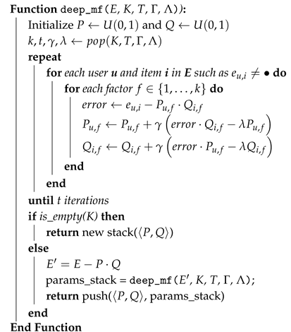
Note that the proposed method consists of successive repetitions of a mf process using the results of the previous mf as input. Therefore, it is possible to make an algorithmic implementation of the proposed method using a recursive approach. Algorithm 1 contains the pseudo-code of the recursive implementation of DeepMF. The algorithm receives as input the E matrix, which contains either the users’ ratings to the items ($R=E^0$) for the first call or the errors of the previous factorization $E^s$ for the successive ones. It also receives the model hyper-parameters: the number of latent factors on each step (K), the number of iterations of the gradient descent optimization on each step (T), the learning rates ($\Gamma$) and the regularizations ($\Lambda$).

Note that these hyper-parameters were stacked so that each of the factorizations performed uses different hyper-parameters. The hyper-parameters of the first factorization will be placed at the top of the stack, those of the second factorization in the next one and so on until the parameters of the deeper factorization, which will be placed at the bottom of the stack. This allows us to define the stopping criteria of the algorithm: as soon as a stack is empty the learning process will be finished. Similarly, the output of the algorithm will be a stack containing the pairs $\langle P,Q\rangle$ with the hidden factors of each of the factorizations carried out.

Algorithm 1: Pseudo-code of a recursive implementation of DeepMF.

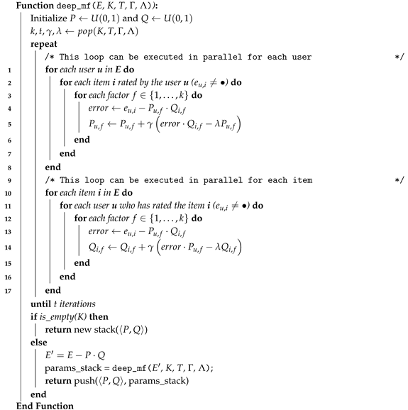
Algorithm 1 needs to be run in a single thread since the update of the P matrix requires the Q matrix and vice versa. However, this algorithm can easily be sped-up by using an Alternating Least Squares (als) approach. Algorithm 2 contains a parrallel implementation of DeepMF using an als approach. As can be observed, to perform a factorization, the matrices P and Q are updated t times according to the loss function gradient. This update is performed in two steps: first, the values of the Q matrix are fixed as constants allowing updating of the latent factors of each user ($P_u$) independently from the latent factors of the rest of the users, thus, they can be updated in parallel for each user. Second, the values of the P matrix are fixed as constants and the latent factors of each item $Q_i$ are updated independently from the latent factors of the rest of the items, thus, they can be updated in parallel for each item. Although this parallel implementation needs to go through the rating set twice to update both the P and the Q matrices, its computation time is significantly less than that of Algorithm 1 when more than 2 execution threads are available. For example, in a dataset with 1 million ratings, the total computation time of each iteration will be the time required to update the Algorithm 2, the total computation time in a processor with 8 execution threads of each iteration will be the time required to update the matrices P and Q 2 * 1 million / 8 threads = 250,000 times, a quarter of the total computation time required by Algorithm 1.

Algorithm 2: Pseudo-code of a parrallel recursive implementation of Deepmf using an als approach.

3. Results

In this section we describe the empirical experiments designed to evaluate the performance of the proposed method. According to the standard cf’s evaluation framework [32], the evaluation of the quality of the predictions is carried out by measuring the Mean Absolute Error (mae) of the model output. The mae is defined as average absolute difference between the actual ratings R and the predicted ratings $\widehat{R}$ of the test split $R^{\mathrm{test}}$:

$$\mathrm{MAE}=\frac{1}{\#R^{\mathrm{test}}}\sum _{\langle u,i\rangle \in R^{\mathrm{test}}}|R_{u,i}-{\widehat{R}}_{u,i}|.$$

(10)

Analogously, the quality of the top l recommendations is evaluated by the precision and recall quality measures on the recommendation lists. Remark that, given an user u, his recommendation list of l items, $L_u^l$, is the collection of the l items $i_1,\dots ,i_l$ with ${\widehat{R}}_{u,i_1},\dots ,{\widehat{R}}_{u,i_l}$ the highest l predicted ratings.

Now, we fix a parameter $\theta \ge 0$, which plays the role of a minimum threshold to discern whether or not an item is of interest to the users. The precision is defined as the average proportion of successful recommendations of the recommendation list:

$$\mathrm{precision}=\frac{1}{\#U^{\mathrm{test}}}\sum _{u\in U^{\mathrm{test}}}\frac{\left\{i\in L_u^l|R_{u,i}\ge \theta \right\}}{l},$$

(11)

where $U^{\mathrm{test}}$ is the collection of users in the test split.

In the same vein, the recall is defined as the averaged proportion of successful recommendations included in the recommendation list with respect to the total number of test items the user u likes:

$$\mathrm{recall}=\frac{1}{\#U^{\mathrm{test}}}\sum _{u\in U^{\mathrm{test}}}\frac{\left\{i\in L_u^l|R_{u,i}\ge \theta \right\}}{\left\{i\in R_u^{\mathrm{test}}|R_{u,i}\ge \theta \right\}},$$

(12)

where $R_u^{\mathrm{test}}$ is the collection of items in the test split at the u-th row of R.

The experimental evaluation has been carried out using MovieLens [33], FilmTrust [34] and MyAnimeList [35] datasets.

Table 1. Main parameters of the datasets used in the experiments.

Dataset	Number of Users	Number of Items	Number of Ratings	Number of Test Ratings	Possible Scores
MovieLens 100K	943	1682	92,026	7974	1 to 5 stars
MovieLens 1M	6040	3706	911,031	89,178	1 to 5 stars
FilmTrust	1508	2071	32,675	2819	0.5 to 4.0 with half increments
MyAnimeList	69,600	9927	5,788,207	549,027	1 to 10

contains their main parameters. To ensure the reproducibility of these experiments, all of them have been run using the benchmark version of these datasets included in Collaborative Filtering for Java (CF4J) [36].

The selection of the baselines has been done trying to pick a representative sample of the existing mf models. A first approach, based on the deep nature of the proposed method, is to focus on existing deep factorization models such as FAuST [25] and DNMF [27]. However recall that, as stated in Section 1, these methods were designed for image processing, not for solving cf problems, so a performance similar to other standard MF-based cf algorithms is not guaranteed. Trying to discern whether these methods would be suitable for cf, we proposed a preliminary experiment for evaluating the performance of FAuST against the MovieLens 100K dataset. To tune the hyper-parameters, a grid search was conducted whose limits are as follows. It was searched for factorizations of the rating matrix R into up to 4 smaller matrices, with 6 or 9 hidden factors for each level and a gradient descent step size (learning rate) of $\gamma =0.0001$ or $0.01$. Notice that FAuST also allows you to impose a sparsity constraint on each factor matrix. For this experiment, it was allowed a $0\%$ of sparsity (i.e., fully dense matrix with no restrictions) or a $20\%$ of sparsity (that is, up to $80\%$ of non-vanishing entries are allowed). The best found model attained a mae of 3.49262 with a factorization into 4 matrices, all with 9 hidden factors, no sparsity constraints and a learning rate of $\gamma =0.01$. This result is very far from the current baselines reported in the literature, which are typically around $0.75$ as we will see below, showing that the existing deep methods are unsuitable as RSs. In is worthy to mention that, although FAuST with no sparsity constraints is very similar to the usual PMF [29] algorithm, it looks for a factorization into normalized matrices with Frobenius norm 1. This normalization seems to be crucial for the bad performance of FAuST as RS: this restriction might be very useful for image processing and memory saving problems which are the usual applications of FAuST, but it seems to be very ill-posed for regression problems.

Due to the failure of this method as RS, it was decided to pull apart the existing deep factorization methods, designed specifically for image processing, and to choose the competing baselines from the most popular MF-based cf methods, namely PMF [29], NMF [30] and SVD++ [31].

These baselines contain several hyper-parameters that must be tuned in order to improve their performance on the selected datasets. The optimal configuration of the hyper-parameters of each baseline has been found by a grid search optimization. All combinations resulting from evaluating a wide range of values for each hyper-parameter have been evaluated, and the combination returning the least mae on the predictions of the test split has been selected as the most suitable for each baseline and data set.

Table 2. Best hyper-parameters for each baseline found by a grid search optimization.

Dataset	PMF	NMF	SVD++
MovieLens 100K	$k=2$, $\gamma =0.01$, $\lambda =0.025$	$k=2$	$k=2$, $\gamma =0.0014$, $\lambda =0.08$
MovieLens 1M	$k=8$, $\gamma =0.01$, $\lambda =0.045$	$k=2$	$k=4$, $\gamma =0.0014$, $\lambda =0.05$
FilmTrust	$k=4$, $\gamma =0.015$, $\lambda =0.1$	$k=2$	$k=2$, $\gamma =0.0014$, $\lambda =0.1$
MyAnimeList	$k=10$, $\gamma =0.005$, $\lambda =0.085$	$k=2$	$k=4$, $\gamma =0.0014$, $\lambda =0.02$

contains the resulting hyper-parameters of this optimization process. Recall that k denotes the number of hidden factors in the factorization, $\gamma$ is the learning rate of the associated gradient descent optimization and $\lambda$ is the regularization hyper-parameter.

Analogously, DeepMF also contains several hyper-parameters needed to fit the model to an specific dataset. As with the baselines, we performed a grid search optimization in order to obtain the combination of parameters that minimizes the prediction error (mae) in the test split. In this case, the recursive nature of the proposed method causes that the number of hyper-parameter combinations to be evaluated grows exponentially.

To deal with this combinatorial explosion, we evaluated with depths from 1 to 4, i.e., performing 1 to 4 deep factorizations. Each of this factorizations has been evaluated varying the number of latent factors $k\in \{3,6,9\}$, the learning rate $\gamma \in \{0.01,0.1\}$ and the regularization $\lambda \in \{0.01,0.1\}$. The number of iterations has been fixed to $T=[50,50,\dots ,50]$ for all factorizations. In total, 22,620 combinations of hyper-parameters has been evaluated for each dataset.

Table 3. Top 5 results resulting from grid search optimization of DeepMF.

Dataset	Rank	Hyper-Parameters	MAE
MovieLens 100K	1	K = [3, 3, 3, 3]; $\Gamma$= [0.01, 0.1, 0.01, 0.1]; $\Lambda$ = [0.1, 0.01, 0.1, 0.01]	0.75017
	2	K = [3, 3, 3, 9]; $\Gamma$= [0.01, 0.1, 0.01, 0.1]; $\Lambda$ = [0.1, 0.01, 0.1, 0.01]	0.75077
	3	K = [3, 6, 6, 3]; $\Gamma$= [0.01, 0.1, 0.01, 0.1]; $\Lambda$ = [0.1, 0.01, 0.1, 0.01]	0.75079
	4	K = [3, 3, 3]; $\Gamma$= [0.01, 0.1, 0.01]; $\Lambda$ = [0.1, 0.01, 0.1]	0.75092
	5	K = [3, 3, 9, 9]; $\Gamma$= [0.01, 0.1, 0.01, 0.1]; $\Lambda$ = [0.1, 0.01, 0.1, 0.01]	0.75105
MovieLens 1M	1	K = [9, 3, 3]; $\Gamma$= [0.01, 0.01, 0.01]; $\Lambda$ = [0.1, 0.01, 0.1]	0.70943
	2	K = [9, 3, 9, 3]; $\Gamma$= [0.01, 0.01, 0.01, 0.1]; $\Lambda$ = [0.1, 0.01, 0.1, 0.01]	0.70948
	3	K = [9, 3, 9]; $\Gamma$= [0.01, 0.01, 0.01]; $\Lambda$ = [0.1, 0.01, 0.1]	0.70949
	4	K = [9, 3, 3, 9]; $\Gamma$= [0.01, 0.01, 0.01, 0.1]; $\Lambda$ = [0.1, 0.01, 0.1, 0.01]	0.70956
	5	K = [9, 3, 3, 3]; $\Gamma$= [0.01, 0.01, 0.01, 0.1]; $\Lambda$ = [0.1, 0.01, 0.1, 0.01]	0.70959
FilmTrust	1	K = [6, 6, 3]; $\Gamma$= [0.01, 0.1, 0.01]; $\Lambda$ = [0.1, 0.01, 0.01]	0.64936
	2	K = [6, 6, 3]; $\Gamma$= [0.01, 0.1, 0.01]; $\Lambda$ = [0.1, 0.01, 0.1]	0.64987
	3	K = [6, 3, 6]; $\Gamma$= [0.01, 0.1, 0.01]; $\Lambda$ = [0.1, 0.01, 0.1]	0.65072
	4	K = [9, 3, 3]; $\Gamma$= [0.01, 0.1, 0.01]; $\Lambda$ = [0.1, 0.01, 0.1]	0.65088
	5	K = [6, 6]; $\Gamma$= [0.01, 0.01]; $\Lambda$ = [0.1, 0.01]	0.65102
MyAnimeList	1	K = [9, 6, 9, 6]; $\Gamma$= [0.01, 0.1, 0.01, 0.1]; $\Lambda$ = [0.1, 0.01, 0.1, 0.01]	0.97447
	2	K = [9, 9, 6, 9]; $\Gamma$= [0.01, 0.1, 0.01, 0.1]; $\Lambda$ = [0.1, 0.01, 0.1, 0.01]	0.97452
	3	K = [9, 6, 6, 6]; $\Gamma$= [0.01, 0.1, 0.01, 0.1]; $\Lambda$ = [0.1, 0.01, 0.1, 0.01]	0.97454
	4	K = [9, 6, 6, 9]; $\Gamma$= [0.01, 0.1, 0.01, 0.1]; $\Lambda$ = [0.1, 0.01, 0.1, 0.01]	0.97454
	5	K = [9, 9, 9, 6]; $\Gamma$= [0.01, 0.1, 0.01, 0.1]; $\Lambda$ = [0.1, 0.01, 0.1, 0.01]	0.97458

contains the top five results returned by the grid search optimization. Note that hyper-parameters has been named as in Algorithm 1 to facilitate their interpretation.

Once all the evaluated models have been set up, the best tuned models can be compared to measure the prediction and recommendation improvement of DeepMF with respect to the selected baselines.

Table 4. Quality of the predictions measured by the mae. The lower the better. In bold the best recommendation model for each dataset.

Dataset	DeepMF	PMF	NMF	SVD++
MovieLens 100K	0.75017	0.76720	0.79138	0.78170
MovieLens 1M	0.70943	0.71868	0.75166	0.74285
FilmTrust	0.64936	0.84659	0.82911	0.65748
MyAnimeList	0.97447	1.10006	1.12025	0.95179

contains the mae of the predictions performed by all the evaluated models. We can observe that the proposed model DeepMF significantly improves the accuracy of predictions with respect to other models in MovieLens 100K, MovieLens 1M and FilmTrust datasets. Similarly, in the MyAnimeList dataset, DeepMF substantially improves PMF and NMF baselines and achieves a slightly worse mae than SVD++. Observe that this later underperformance might be due to the fact that MyAnimeList is significantly larger than any other dataset, so deeper models of DeepMF would be needed in order the exploit the recursive nature of the proposed method that fit the dataset better than SVD++.

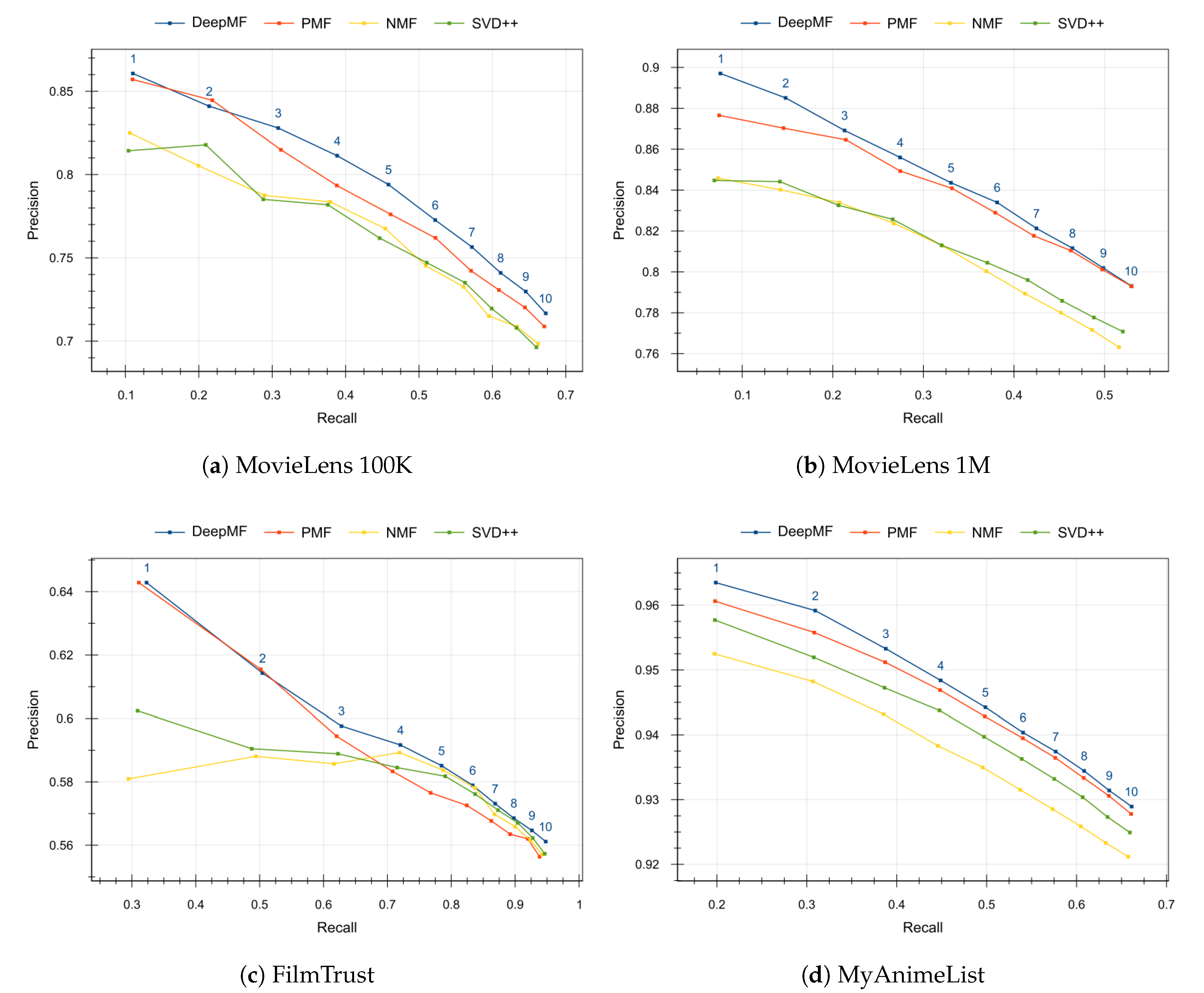
Figure 2 contains the precision and recall of the recommendations when varying the number of desired top recommendations from $l=1$ to $l=10$ items. The threshold $\theta$ for precision and recall has been set to $\theta =4$ for MovieLens datasets, $\theta =3.5$ for FilmTrust dataset and $\theta =7$ for MyAnimeList dataset. We can observe that in all evaluated datasets the proposed method DeepMF provides the best balance between the precision and recall quality measures for any number of recommendations.

All experiments conducted in this article are committed to reproducible science. The full code of these experiments is available at https://github.com/ferortega/deep-matrix-factorization.

4. Discussion

In this paper, we presented DeepMF, a novel MF-based cf algorithm using a dl approach. As stated in Section 1 the dl is an incipient approach in the ml field that consists of a hierarchical self-training method that uses the information acquired from data. Although dl has been used mainly in artificial neural networks, the proposed model breaks this tendency by applying the foundations of dl to the field of MF.

The essence of the proposed method lies in the dl approach. Our model performs successive matrix factorizations in order to successively refine the model output. Thus, the first factorization, the least deep one, represents the classic approach of mf-based cf models and seeks to predict the score that a user will give to an item. The second factorization seeks to refine the previous prediction by trying to increase the predictions that tend to be lower than the real rating and decrease those that tend to be higher. Subsequently, the learning is deepened by correcting the errors of the errors to build a dl model that converges towards a prediction as close as possible to the real value to be learned.

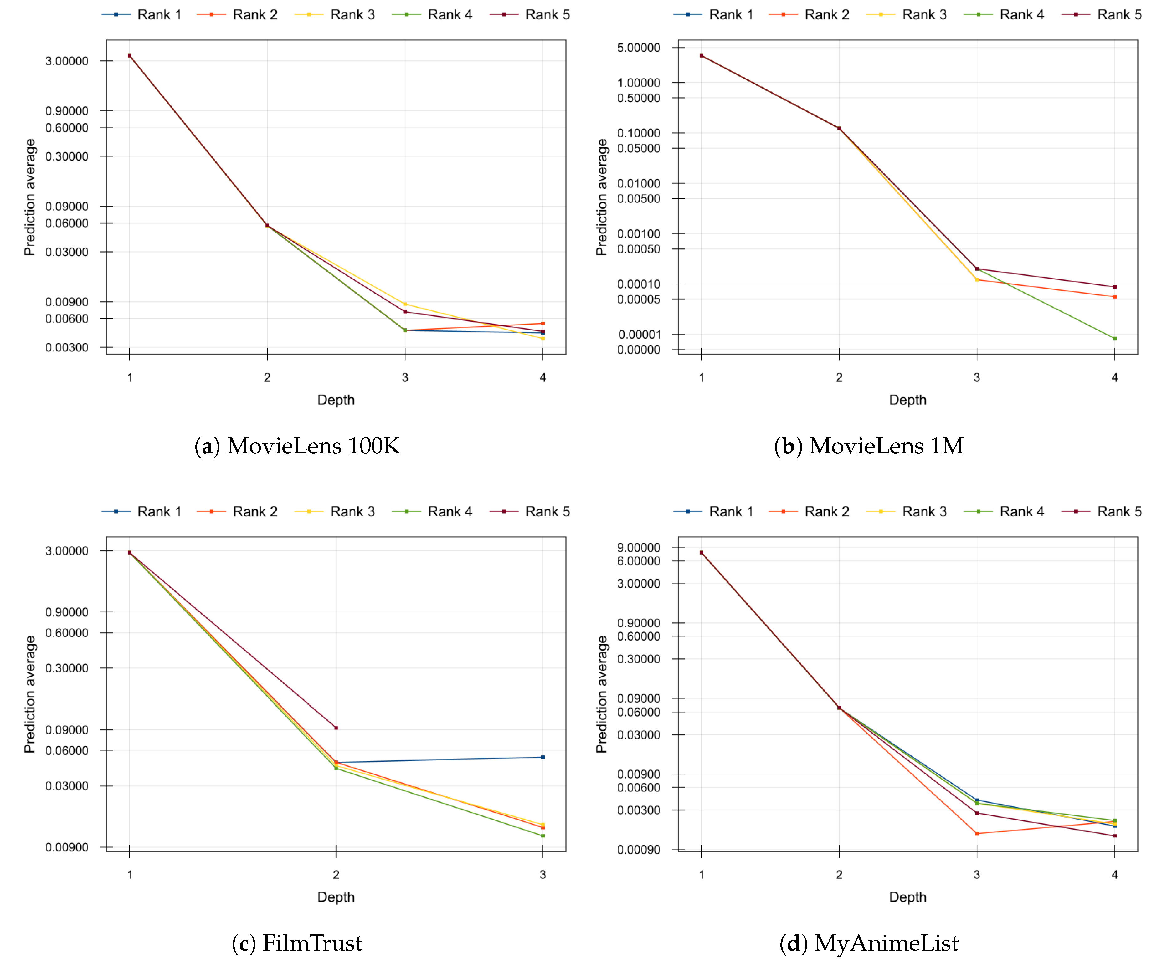
This expected behavior is corroborated by the results of the experiment shown in Figure 3. On it, we plot the average value of the predictions provided by each factorization layer according to its depth. The same decreasing trend in the average prediction is observed in all the analyzed datasets: as factorization is deeper, errors to be refined tend to zero and the learning process converges. The Figure 3 includes the top 5 combinations of hyper-parameters obtained in the grid search shown in Table 3. Note that a logarithmic scale has been used on the y-axis to emphasize the differences in the deeper factorizations.

The hypothesis of this contribution was that a dl approach applied to a mf-based cf can improve the quality of both predictions and recommendations. This hypothesis has been confirmed with the experimental results showed in Section 3. The quality of the predictions (see Table 4) and recommendations (see Figure 2) of the proposed method, DeepMF, exceeds the baselines used in the 3 datasets analyzed: MovieLens 100K, MovieLens 1M and FilmTrust.

Summarizing, the proposed model in this paper expands the landscape of matrix factorization models by importing a Deep Learning approach from the field of neural computing. From this point, several future research lines open. Maybe, the most obvious one would be to analyze the dl approach performed in this paper with other matrix factorization models and to define different loss functions depending on the depth of factorization. For example, experimental results show that SVD++ factorization works properly on MyAnimeList dataset, so it would be interesting to evaluate the performance of DeepMF using SVD++ as the initial factorization and other factorizations models for the deeper factorizations.

A more ambitious prospective work would be transferring the ideas of this paper to a purely bioinspired framework. For instance, it can be studied the incorporation of DeepMF as a model to be implemented by the neurons of a fully connected or convolutional neural network. In this way, the knowledge of the scientific community about network architectures can be applied to give rise to deeper an more involved nested patterns of matrix factorizations.