A Multistage Sustainable Production–Inventory Model with Carbon Emission Reduction and Price-Dependent Demand under Stackelberg Game

Abstract

This paper investigated a multistage sustainable production–inventory model for deteriorating items (i.e., raw materials and finished goods) with price-dependent demand and collaborative carbon reduction technology investment under carbon tax regulation. The model was developed by first defining the total profit of the supply chain members under carbon tax regulation and, second, considering a manufacturer (leader)–retailer (follower) Stackelberg game. The optimal equilibrium solutions that maximize the manufacturer’s and retailer’s total profits were determined through the method analysis. An algorithm complemented the model to determine the optimal equilibrium solutions, which were then treated with sensitivity analyses for the major parameters. Based on the numerical analysis, (a) carbon tax policies help reduce carbon emissions for both the manufacturer and retailer; (b) most carbon emissions from supply chain operations negatively impact the total profits of both members; (c) the retailer may increase the optimal equilibrium selling price to respond to an increase in carbon emissions from supply chain operations or carbon tax; and (d) autonomous consumption positively affects both members’ optimal equilibrium policies and total profits, whereas induced consumption does the opposite. These findings are very managerial and instructive for companies seeking profits and fulfilling environmental responsibility and governments.

1. Introduction

Carbon emissions from supply chain logistics processes significantly contribute to climate deterioration. In 2005, with the implementation of the so-called Kyoto Protocol, governments and environmental organizations initiated their active commitment to the adoption of policies and technical measures for carbon emission reduction. Such a dynamic start ignited the emergence of concepts, such as green policies, green energy, and green supply chains. In 2015, the United Nations Framework Convention on Climate Change was settled at the 21st Conference of the States Parties in Paris, France, which promoted the development of alternative and renewable energy sources, as well as the establishment of energy-saving and carbon reduction regulations, as time went by. With the trend now concentrated on carbon emission reduction, there was gradual unification on the carbon reduction policies and enterprises’ profits of production management set by the government. Enterprises came into conjunction with the government policies and regulations for carbon emission reduction, promoting a balance between each entity on strategic decisions to maximize profit objectives under carbon reduction constraints [1]. Through the balance, green production–inventory management complemented the traditional economic focus with environmental protection considerations [2], where companies can significantly reduce carbon emissions through production–inventory management strategies without significantly increasing costs [3]. Therefore, there is a potential for green inventory management practices to reduce both the costs and emissions, at least in terms of the development of practical and more generally sustainable production–inventory models.

Carbon emission and carbon footprint management have increasingly been subjects of discussion in the context of supply chain management. Many existing studies have discussed carbon emission reduction policies, including carbon emissions limitation, carbon tax, carbon quotas, carbon cap-and-trade, and carbon offset. However, most of the studies consider carbon emissions as exogenous changes. In real life, enterprises can invest in processes, i.e., product design, production, inventory, and transportation activities, to effectively reduce carbon emissions. Most enterprises can focus on carbon emission reduction via several physical processes and investments, such as replacing energy-efficient equipment or facilities, redesigning product packaging and scheduling, and using energy sources with low pollution [4]. Though companies can invest in green technologies in each emission source to reduce emissions [5,6], a large amount of money may be needed. Thus, from a supply chain perspective, it is more rewarding if all members of the supply chain agree on shared investment funds for the relevant facilities and enjoy the benefits of low carbon emissions, minimal costs, and increased profits. Thus, this study introduces co-investment for carbon reduction technology, which is rarely considered.

In a supply chain system, members’ decisions regarding manufacturing, stocking, and investments may influence one another. Previous studies focused mostly on the equal decision-making power of participating merchants in the supply chain. However, if the participants have unequal power and there is a dependency and restriction relationship between each other’s decisions, then a game strategy is more useful. Game theory is a useful and attractive method for the resolution of interactive decisions and has thus been adopted by various studies for the discussion of interactive decisions [7].

On the basis of the above, in actual supply chain systems, it also needs to be considered that the demand rate is often dictated by the selling price. However, presently, there is no discussion on a production–inventory model considering carbon reduction technology co-investment and price-dependent demand from the perspective of the game theory. Therefore, this study investigates a multistage sustainable production–inventory model for deteriorating items under carbon tax policy, where the cooperation form between the manufacturer and retailer follows the rules of the Stackelberg game and where demand rate is assumed to be a function of the selling price. The objective is to determine the retailer’s optimal replenishment and pricing policies, as well as the manufacturer’s production and investing policies, which maximize the profits of both parties under Stackelberg equilibrium.

The proposed model is innovative and unique due to the reasons: (1) Most of the previous production–inventory models only discussed the inventory of finished products, but did not consider the raw materials—the current model includes both materials and finished products inventory; (2) this model suggests that both the manufacturer and retailer can agree on a joint investment in carbon emission reduction technology and share the benefits of reduced emissions under the carbon tax collection policy; (3) unlike the integrated production–inventory model, the proposed model considers the roles of the manufacturer as the leader and the retailer as the follower from the perspective of the Stackelberg game, as well as the optimal ordering, selling price, shipping, and investment decisions of both parties as the equilibrium is reached. In the mode-solving part, it will be proved that the follower’s optimal solution exists and is unique, after which an algorithm will be developed to find the optimal solution of both parties to achieve Stackelberg equilibrium. Finally, according to an approximate actual situation, under the given mode parameters, mathematical software (Mathematica 12.0) is used to solve and for sensitivity analysis.

The rest of this paper is organized as follows. A brief review of the related literature follows in Section 2. The notations and assumptions used throughout are listed in Section 3. In Section 4, we establish the formula system and develop the theory to obtain the optimal solution. In Section 5, computational results are presented to explain the solution process and investigate the parameter changes on the optimal solution. Finally, conclusions and suggestions are provided in Section 6.

2. Literature Review

2.1. Inventory Model Introducing Carbon Emissions Management

A huge number of studies already exist on inventory models related to carbon emissions and carbon footprint management issues. Chen et al. [4], Hua et al. [8], Battini et al. [9], Hovelaque and Bironneau [10], Liao and Deng [11], Tao and Xu [12], and Daryanto et al. [13] employed the traditional economic order quantity (EOQ) model to develop sustainable batch-order models under different carbon emission policies. More recent studies considered the impacts of carbon emissions and policies on production–inventory issues. Jiang et al. [14] proposed a green vendor-managed inventory model with a supplier and a manufacturer under a carbon emission trading mechanism. Chen et al. [15] investigated how the retailer adjusts optimal ordering policy carbon emissions and total costs under a trade credit and cap-and-trade system, demonstrating that under such a system, the retailer’s total cost depends on the combination of carbon cap allocated to the retailer and the carbon price. Ghosh et al. [16,17] considered a strict carbon cap and carbon tax policy to determine the optimal order quantity, reorder point, and number of shipments in a two-echelon supply chain with stochastic demand. Moreover, Shaw et al. [18] discussed an integrated inventory model between a vendor and a buyer for deteriorating items with defective products and carbon emissions from every portion of the supply chain system. Wee and Daryanto [19] investigated a low-carbon two-echelon supply chain inventory model considering supply chain integration and imperfect quality items when shortages are allowed. Recently, Xu et al. [20] analyzed the impacts of carbon emissions on an inventory system for deteriorating items where a general time-varying demand and shortages are considered.

2.2. Inventory Model Based on Price-Dependent Demand

In reality, a drop in the selling price will often equate to a significant increment in the demand rate [21]; conversely, an increase in the selling price will most likely decrease the market demand. Relevant studies [22,23,24,25,26] consider demand rate as a function of the selling price, which could be described in various inventory models. Jabbarzadeh et al. [27] established a multi-item inventory and pricing model, considering marketing, service activities, trade credit, carbon emissions, and restrictions of production cost and storage space where the demand rate is a power function of service, marketing costs, and selling price. From an analysis of a single item that can be produced in different qualities, Datta et al. [5] revealed that demand rate is quality-dependent, being mainly price-sensitive on each quality.

2.3. Inventory Model Applying Game Theory

The game theory was originally proposed by Hungarian John von Neumann and Princeton economist Morgenstern in 1944. Later, Nash [28] raised a non-cooperative game model, formulating the famous Nash Equilibrium. A Stackelberg game is a two-stage complete information dynamic game where the game time is sequential. Here, the main idea is that both parties choose their own strategies according to each other’s possible strategies in order to ensure that their own profit under the other party’s strategies is maximized [29]. The concept of game theory is well incorporated in some production–inventory models. Emmons and Gilbert [7] formulated an inventory model in which decisions are governed by the Stackelberg game theory. Moreover, they discussed an approach to determine the manufacturer’s wholesale price and the best order quantity determined by the retailer. Hsiao and Lin [30] discussed a traditional EOQ model on the Stackelberg game. Liou et al. [31] considered a one-buyer-and-one-vendor inventory model that introduces the Stackelberg equilibrium framework to maximize the vendor’s total benefit subject to the minimum total cost. Chern et al. [32] derived the necessary and sufficient conditions to obtain the optimal solution for both the vendor and buyer under the non-cooperative Nash equilibrium. Jaggi et al. [33] incorporated deteriorating items to obtain optimal inventory and credit decisions using the Stackelberg and Nash equilibrium solutions. Tao [34] studied the optimization problem for a two-stage supply chain under a decentralized decision-making mode that allowed the formulation of the problem as a Stackelberg game model, where the manufacturer and retailer were the leader and follower, respectively. Zhang et al. [35] established a three-stage pricing model with a third-party logistic enterprise as the leader, whereas the retailer and the consumer were the followers.

2.4. Research Gap Analysis

Table 1. Major characteristics of inventory models in relevant researches.

References	Model	Demand	Carbon Emission	Carbon Emission Reduction Technology	Game Theory Application
Chen et al. [4], Hua et al. [8], Battini et al. [9], Hovelaque & Bironneau [10], Tao & Xu [12], Daryanto et al. [13]	EOQ	Constant	V
Datta et al. [5]	Supply chain	Price-dependent	V	V
Emmons & Gilbert [7], Breton et al. [30]	EOQ	Constant			V
Liao & Deng [11]	EOQ	Uncertain	V
Jiang et al. [14] Chen et al. [15], Shaw et al. [18], Wee & Daryanto [19]	Supply chain	Constant	V
Ghosh et al. [16,17]	Supply chain	Stochastic	V
Xu et al. [20]	Supply chain	Time-varying	V
Panda et al. [21]	EOQ	Price-dependent
Ruidas et al. [22]	EPQ	Price-dependent
Sahoo et al. [23], Li et al. [24], Rahman et al. [25], Sinha et al. [26]	Supply chain	Price-dependent
Jabbarzadeh et al. [27]	Supply chain	Price-dependent	V
Liou et al. [31], Chern et al. [32]	Supply chain	Constant			V
Jaggi et al. [33]	Supply chain	Inventory- dependent			V
Tao [34]	Supply chain	Constant	V		V
Zhang et al. [35]	Multistage Supply chain	Constant			V
This paper	Multistage Supply chain	Price-dependent	V	V	V

Note: Economic Order Quantity (EOQ), Economic Production Quantity (EPQ).

reveals the main differences between this study and above-mentioned existing relevant studies. According to Table 1, although studies have developed various inventory models of carbon emission reduction policies, few have included the investment factors of carbon emission reduction technology, and no study has proposed using the concept of co-investment agreements. Similarly, few studies have used game theory to discuss the interdependent decision-making of supply chain members under the constraints of carbon emission reduction regulations. At the same time, there is no research on the production–inventory model that combines the above two points and the price-dependent demand assumption. The main contribution of this study is that it is the first to apply game theory (Stackelberg game, where the manufacturer is the leader and the retailer is the follower) perspective to discuss an interactive decision-making of the pricing, production, replenishment, and the co-investment in carbon emission reduction technology between manufacturers and retailers with price-dependent demand and multistage issues of raw materials and finished products inventories.

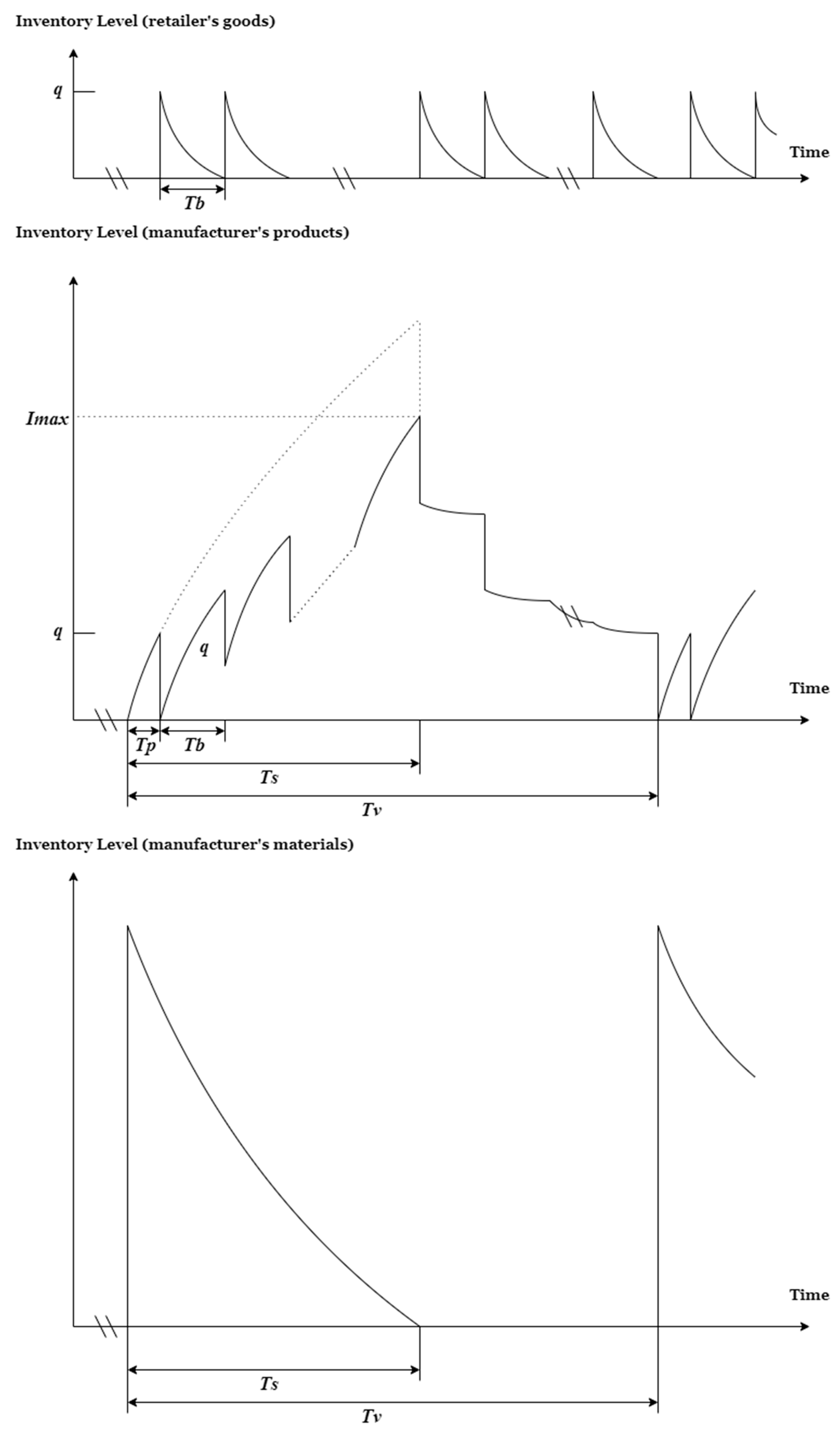
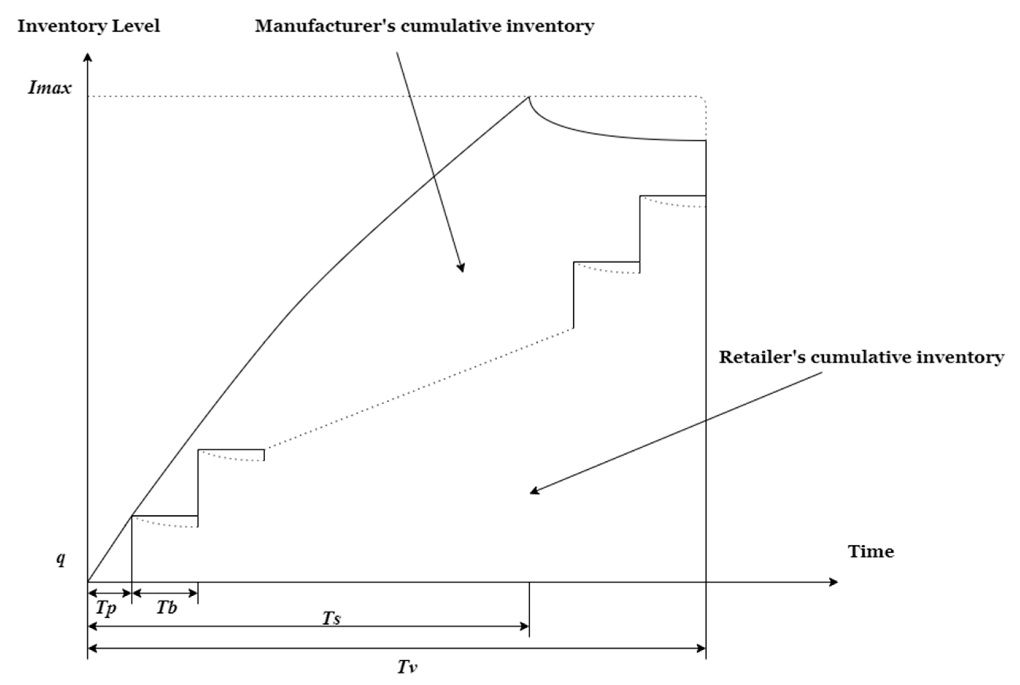
3. Notations and Assumptions

The notations and assumptions below were utilized to develop the multistage sustainable production–inventory model:

3.1. Notations

$P$	Manufacturer’s production rate
$A_R$	Retailer’s ordering cost of finished products per order
${\widehat{A}}_R$	Amount of fixed carbon emissions per order for the retailer
$A_M$	Manufacturer’s ordering cost of raw material per order
${\widehat{A}}_M$	Amount of fixed carbon emissions per order for the manufacturer
$r$	Amount of raw materials required to produce one unit of finished product
$S$	Manufacturer’s setup cost per production cycle
$\widehat{S}$	Amount of fixed carbon emissions per setup for the manufacturer
$c_1$	Manufacturer’s unit raw material cost
${\widehat{c}}_1$	Amount of associated carbon emissions per unit of raw material procurement for the manufacturer
$c_2$	Manufacturer’s unit production cost
${\widehat{c}}_2$	Amount of associated carbon emissions per unit of production for the manufacturer
$v$	Retailer’s unit purchase price at the manufacturer
$\widehat{v}$	Amount of associated carbon emissions per unit of purchase for the retailer
$h_b$	Retailer’s holding cost of finished goods per unit per unit time
${\widehat{h}}_b$	Amount of carbon emissions per unit of finished goods held per unit time for the retailer
$h_m$	Manufacturer’s holding cost of raw material per unit per unit time
${\widehat{h}}_m$	Amount of carbon emissions per unit of raw material held per unit time for the manufacturer
$h_v$	Manufacturer’s holding cost of finished goods per unit per unit time
${\widehat{h}}_v$	Amount of carbon emissions per unit of finished goods held per unit time for the manufacturer
$C_T$	Retailer’s fixed shipping cost per shipment
${\widehat{C}}_T$	Amount of fixed carbon emissions per shipment for the retailer
$C_t$	Retailer’s variable shipping cost per unit
${\widehat{C}}_t$	Amount of associated carbon emissions per unit shipped for the retailer
$C$	Carbon tax per unit of carbon emission
${\theta }_1$	Carbon deterioration rate of the raw material
${\theta }_2$	Deterioration rate of the finished goods
$p$	Retailer’s unit selling price
$D\left(p\right)$	Demand rate, which is dependent on the unit selling price $p$
$\varpi$	Technology investment for carbon emission reduction
$m\left(\varpi \right)$	Proportion of reduced carbon emissions as a function of $\varpi$
$Q$	Retailer’s order quantity
$n$	Number of shipments from the manufacturer to the retailer during a production cycle
$q$	Quantity shipped from the manufacturer to the retailer per shipment
$T_b$	Length of the retailer’s replenishment cycle
$T_v$	Length of the manufacturer’s production cycle
$T_s$	Length of the manufacturer’s production period per production cycle
$T_p$	Length of period for the manufacturer to manufacture and deliver the first batch of finished products to the retailer
$**$	The superscript represents the optimal equilibrium value.

3.2. Assumptions

• The sustainable multistage supply chain system considers a single manufacturer, single retailer, single material, and single commodity under carbon tax regulation.
• The demand rate $D\left(p\right)$ is a non-negative continous function of the selling price (Please refer to Yang et al. [36]).
• The manufacturer production rate is finite and greater than the demand rate, i.e., $P>D\left(p\right)$; otherwise, no inventory problems would occur.
• Operational activities, such as ordering, holding inventory of finished goods, shipping, and purchasing, are the source of carbon emissions produced by the retailer. On the manufacturer’s part, the source includes operations, such as purchase of materials, setting up, production, and holding inventories of raw material and finished goods (Please refer to Shaw et al. [18]).
• Based on Ghosh et al. [17], carbon tax is levied on the manner by which carbon is emitted—that is, it is in the form of a unit tax in the proposed model.
• Carbon emissions can be reduced by investments in technology, at a proportion defined by the reduced rate $m\left(\varpi \right)$, where $1<m\left(\varpi \right)<1$, and $m\left(\varpi \right)$ is an increasing function of $\varpi$.
• Both the manufacturer and retailer share in the technological investment to reduce carbon emission, according to capital investment proportions $\beta$ (retailer) and $1-\beta$ (manufacturer), where $0\le \beta \le 1$.
• Shortages are not allowed for either the manufacturer or the retailer to avoid losing customers (Chen et al. [4]).

4. Model Formulation and Solution

In the proposed multistage sustainable production–inventory model with carbon emission reduction investment and price-dependent demand employing the Stackelberg game decision-making approach under carbon tax regulation, three stages form the supply chain process: (a) raw material supply, (b) production delivery, and (c) order sales. Figure 1 presents a diagram of the production, delivery, and sales process of the supply chain system. In a single-manufacturer–single-retailer system, the manufacturer acts as the leader, whereas the retailer acts as the follower. Here, the retailer places $Q$ units per order with the manufacturer, and the manufacturer delivers the order in $n$ batches (with the freight cost shouldered by the retailer). First, the manufacturer fulfills the retailer’s order by purchasing raw materials from an original supplier. Next, when the production quantity reaches $q$ units for the first time (after a period $T_p$), the manufacturer begins shipping the materials to the retailer to comply with the just-in-time (JIT) inventory system. Successive shipments of $q$ quantities are then shipped in regular intervals (or after periods $T_b$). When the production rate exceeds the demand rate, the manufacturer may stop the production as soon as the quantity reaches $I_{max}$ (after a period $T_S$) but continues the regular shipments until the entire order is fulfilled. The inventory levels of the manufacturer’s materials and products and the retailer’s goods in a complete production cycle are presented in Figure 2.

Based on the above notations and assumptions, the retailer’s and manufacturer’s total profits per unit time with carbon tax regulation were established as follows.

4.1. Retailer’s Total Profit with Carbon Tax

The retailer’s inventory level of finished goods at time $t$ during the replenishment cycle changes due to a price-dependent demand and the deterioration of the finished goods, as represented by the differential equation:

$$d{I}_R\left(t\right)/dt+{\theta }_2{I}_R\left(t\right)=-D\left(p\right),0\le t\le T_b.$$

(1)

Assuming the boundary condition $I_R\left(T_b\right)=0$, Equation (1) transforms into:

$$I_R\left(t\right)=\frac{D\left(p\right)}{{\theta }_2}\left[e^{{\theta }_2\left(T_b-t\right)}-1\right],0\le t\le T_b,$$

(2)

where the quantity shipped by the manufacturer to the retailer per shipment $q$ can be described by:

$$q=I_R\left(0\right)=\frac{D\left(p\right)}{{\theta }_2}\left(e^{{\theta }_2{T}_b}-1\right)$$

(3)

The retailer’s total profit per unit time is determined by sales revenue, ordering cost, purchasing cost, transportation cost, holding cost, and carbon emission reduction investment, which are evaluated as follows:

(a)

The sales revenue per unit time is $PD\left(P\right)$

(b)

The ordering cost per unit time is $A_R/T_b$

(c)

The retailer’s purchasing cost per unit time is:

$$\frac{vq}{T_b}=\frac{vD\left(p\right)}{{\theta }_2{T}_b}\left(e^{{\theta }_2{T}_b}-1\right)$$

(d)

The retailer’s transportation cost consists of fixed and variable costs per unit time and is given by:

$$\frac{C_T+C_{t}q}{T_b}=\frac{C_T}{T_b}+\frac{C_{t}D\left(p\right)}{{\theta }_2{T}_b}\left(e^{{\theta }_2{T}_b}-1\right)$$

(e)

The retailer’s holding cost per unit time is:

$$\frac{h_b}{T_b}{{\displaystyle \int }}_0^{T_b}{I}_R\left(t\right)dt=\frac{h_b}{T_b}{{\displaystyle \int }}_0^{T_b}\frac{D\left(p\right)}{{\theta }_2}\left[e^{{\theta }_2\left(T_b-t\right)}-1\right]dt=\frac{h_{b}D\left(p\right)}{{\theta }_2^2{T}_b}\left(e^{{\theta }_2{T}_b}-{\theta }_2{T}_b-1\right)$$

(f)

The technological investment in carbon emission reduction is $\varpi$. Because the technology investment is shared between the retailer and manufacturer, with $\beta \left(0\le \beta \le 1\right)$ being the proportion of the retailer’s investment, the investment reduces the carbon emission per unit time for the retailer as indicated by $\mathit{\beta \varpi }$.

Considering the points above, the retailer’s total profit per unit time can be formulated as:

$$T{P}_b\left(p,T_b\right)=pD\left(p\right)-\frac{1}{T_b}\left[A_R+C_T+\frac{\left(C_t+v\right)D\left(p\right)}{{\theta }_2}\left(e^{{\theta }_2{T}_b}-1\right)+\frac{h_{b}D\left(p\right)}{{\theta }_2^2}\left(e^{{\theta }_2{T}_b}-{\theta }_2{T}_b-1\right)\right]-\beta \varpi$$

(4)

Subsequently, the amount of carbon emissions produced by the retailer per unit time is relative to the ordering, transportation, purchase, and holding inventory; thus, it can be reduced through investment in carbon emission technology. At a reduction rate of the total carbon emissions $m\left(\varpi \right)$, the amount of carbon emissions produced by the retailer per unit time is defined as:

$$E_b\left(p,T_b\right)=\frac{\left[1-m\left(\varpi \right)\right]}{T_b}\left[{\widehat{A}}_R+{\widehat{C}}_T+\frac{\left({\widehat{C}}_t+\widehat{v}\right)D\left(p\right)}{{\theta }_2}\left(e^{{\theta }_2{T}_b}-1\right)+\frac{{\widehat{h}}_{b}D\left(p\right)}{{\theta }_2^2}\left(e^{{\theta }_2{T}_b}-{\theta }_2{T}_b-1\right)\right].$$

(5)

With the carbon tax regulation, the retailer pays a C amount of money for each unit of carbon emitted [37]. Hence, the retailer’s total profit per unit time with carbon tax is represented by:

$$\begin{gathered} T{P}_{CTb}\left(p, T_b\right)=T{P}_b\left(p, T_b\right)-C{E}_b\left(p, T_b\right) \\ \begin{array}{cc}\hfill =pD\left(p\right)-\frac{1}{T_b}& {\displaystyle \{}\left(A_R+C_T\right)+\left[1-m\left(\varpi \right)\right]\left({\widehat{A}}_R+{\widehat{C}}_T\right)\hfill \\ & +\frac{\left\{\left(C_t+v\right)+\left[1-m\left(\varpi \right)\right]\left({\widehat{C}}_t+\widehat{v}\right)\right\}D\left(p\right)}{{\theta }_2}\left(e^{{\theta }_2{T}_b}-1\right)\hfill \\ & +\frac{\{h_b+\left[1-m\left(\varpi \right)\right]{\widehat{h}}_b\}D\left(p\right)}{{\theta }_2^2}\left(e^{{\theta }_2{T}_b}-{\theta }_2{T}_b-1\right){\displaystyle \}}-\beta \varpi .\hfill \end{array} \end{gathered}$$

(6)

4.2. Manufacturer’s Total Profit with Carbon Tax

Figure 2 presents the manufacturer’s inventory level of raw materials in a complete production cycle. In the cycle, upon receipt of the retailer’s order ($Q$ units), the manufacturer purchases raw materials from an original material supplier. Assuming that one unit of the finished product requires r units of raw materials and the materials deteriorate during storage, the manufacturer’s inventory level fluctuates, with respect to the use of materials for production and to the deterioration of the materials during the time interval $\left[0,T_s\right]$. As such, the inventory level changes at time t within $\left[0,T_s\right]$, which can be represented in the differential equation:

$$d{I}_M\left(t\right)/dt+{\theta }_1{I}_M\left(t\right)=-rP,0\le t\le T_s$$

(7)

Assuming the boundary condition $I_M\left(T_s\right)=0$, the manufacturer’s inventory level of materials per production cycle is given by:

$$I_M\left(t\right)=\frac{rP}{{\theta }_1}\left[e^{{\theta }_1\left(T_s-t\right)}-1\right],0\le t\le T_S,$$

(8)

from which the total amount of raw materials per production cycle $q_M$ is:

$$q_M=I_M\left(0\right)=\frac{rP}{{\theta }_1}\left(e^{{\theta }_1{T}_s}-1\right).$$

(9)

To comply with JIT, the manufacturer delivers products to the retailer immediately at the start of the production cycle while producing $q=Q/n$ units of the finished products. Moreover, regular shipments of fixed quantity ($q$units) are made in succession every $T_b$ until the n number of shipments per production cycle is fulfilled (Figure 2).

Accordingly, the manufacturer’s inventory level of finished goods changes due to the production and deterioration of items within $\left[0,T_s\right]$. Because the production rate exceeds the demand rate, the manufacturer stops the production after a certain inventory level $I_{max}$ is achieved and then gradually decreases with the deterioration of finished goods during $\left[T_s,T_v\right]$. On the other hand, the manufacturer delivers products to the retailer for n times throughout the time period $\left[0,T_v\right]$. The manufacturer’s and retailer’s cumulative inventory of finished goods is presented in Figure 3.

The manufacturer’s inventory level of finished goods at time t during the time interval $\left[0,T_s\right]$ is governed by the differential equation:

$$d{I}_p\left(t\right)/dt+{\theta }_2{I}_p\left(t\right)=P,0\le t\le T_s$$

(10)

Assuming $I_p\left(0\right)=0$, the manufacturer’s inventory level of finished goods becomes:

$$I_P\left(t\right)=\frac{P}{{\theta }_2}\left(1-e^{-{\theta }_{2}t}\right),0\le t\le T_S$$

(11)

After completing the first $q$ units at time $T_p$, the manufacturer immediately ships the products to the retailer. This is governed by the relation $I_P\left(T_p\right)=q=\frac{D\left(p\right)}{{\theta }_2}\left(e^{{\theta }_2{T}_b}-1\right)$ from Equation (3), implying that:

$$T_p=\frac{1}{{\theta }_2}\ln \left[\frac{P}{P-D\left(p\right)\left(e^{{\theta }_2{T}_b}-1\right)}\right]$$

(12)

Thus, at $\left[T_s,T_v\right]$, the manufacturer no longer produces, which results in a drop in the inventory level due to material deterioration. At a certain time t, the inventory level of the finished goods is governed by the rule:

$$d{I}_d\left(t\right)/dt+{\theta }_2{I}_d\left(t\right)=0,T_s\le t\le T_v$$

(13)

Assuming the boundary condition $I_d\left(T_v\right)=nq=\frac{nD\left(p\right)}{{\theta }_2}\left(e^{{\theta }_2{T}_b}-1\right)$, Equation (13) can be solved to determine the inventory level during the interval $\left[T_s,T_v\right]$, which is given by:

$$I_d\left(t\right)=\frac{nD\left(p\right)}{{\theta }_2}\left(e^{{\theta }_2{T}_b}-1\right)e^{{\theta }_2\left(T_v-t\right)},T_s\le t\le T_v$$

(14)

Manipulating Equations (11) and (14) and assuming $I_p\left(T_s\right)=I_d\left(T_s\right)$, the manufacturer’s production period per production cycle can be solved using the equation:

$$T_s=\frac{1}{{\theta }_2}\ln \left[\frac{P+nD\left(p\right)\left(e^{{\theta }_2{T}_b}-1\right)e^{{\theta }_2{T}_v}}{P}\right]$$

(15)

With respect to the manufacturer’s total profit per unit time, its components include the sales revenue, setup cost, ordering cost, material cost, production cost, defective item processing cost, and holding cost, which are evaluated as follows:

(a)

The manufacturer’s sales revenue per unit time is:

$$\frac{vQ}{\left(T_v+T_b\right)}=\frac{vnq}{\left(T_v+T_b\right)}=\frac{vnD\left(p\right)}{{\theta }_2\left(T_v+T_b\right)}\left(e^{{\theta }_2{T}_b}-1\right)$$

(b)

The manufacturer’s setup cost per unit time is $S/\left(T_v+T_b\right)$.

(c)

The manufacturer’s ordering cost for material per unit time is $A_M/\left(T_v+T_b\right)$.

(d)

The manufacturer’s material cost per unit time is:

$$\frac{c_1{q}_M}{\left(T_v+T_b\right)}=\frac{c_{1}rP}{{\theta }_1\left(T_v+T_b\right)}\left(e^{{\theta }_1{T}_s}-1\right)$$

(e)

The manufacturer’s production cost per unit time is:

$$\frac{c_{2}P{T}_s}{\left(T_v+T_b\right)}=\frac{c_{2}P}{{\theta }_2\left(T_v+T_b\right)}\ln \left[\frac{P+nD\left(p\right)\left(e^{{\theta }_2{T}_b}-1\right)e^{{\theta }_2{T}_v}}{P}\right]$$

(f)

The manufacturer’s holding cost is computed from the raw materials and the finished goods. The holding cost of the raw materials per unit time is:

$$\frac{h_m}{\left(T_v+T_b\right)}{{\displaystyle \int }}_0^{T_s}{I}_M\left(t\right)dt=\frac{h_{m}rP}{{\theta }_1^2\left(T_v+T_b\right)}(e^{{\theta }_1{T}_s}-{\theta }_1{T}_s-1).$$

With respect to the holding cost of the finished goods, the manufacturer’s total inventory per unit time is equal to the manufacturer’s cumulative inventory minus the retailer’s cumulative inventory (see Figure 3), which is given by ${{\displaystyle \int }}_0^{T_s}{I}_p\left(t\right)dt+{{\displaystyle \int }}_{T_s}^{T_v}{I}_d\left(t\right)dt-q{T}_b\left[1+2+\cdots +\left(n-1\right)\right]$. Thus, the holding cost of the finished goods is:

$$\begin{gathered} \frac{h_v}{\left(T_v+T_b\right)}\left\{{{\displaystyle \int }}_0^{T_s}{I}_p\left(t\right)dt+{{\displaystyle \int }}_{T_s}^{T_v}{I}_d\left(t\right)dt-q{T}_b\left[1+2+\cdots +\left(n-1\right)\right]\right\} \\ =\frac{h_v}{\left(T_v+T_b\right)}\{\frac{P}{{\theta }_2{}^2}\left(e^{-{\theta }_2{T}_s}+{\theta }_2{T}_s-1\right)+\frac{nD\left(p\right)}{{\theta }_2{}^2}\left(e^{{\theta }_2{T}_b}-1\right)\left[e^{{\theta }_2\left(T_v-T_s\right)}-1\right] \\ -\frac{n\left(n-1\right)D\left(p\right)T_b}{2{\theta }_2}\left(e^{{\theta }_2{T}_b}-1\right)\} \end{gathered}$$

(g)

As in the case of the retailer, the technological investment in carbon emission reduction is $\varpi$. Because the investment is shared between the two players, with the proportion of the manufacturer’s being at $1-\beta \left(0\le \beta \le 1\right)$, the investment reduces the carbon emission per unit time for the manufacturer by $\left(1-\beta \right)\varpi$.

Consequently, the manufacturer’s total profit per unit time is given by:

$$\begin{gathered} T{P}_v\left(T_v,T_s,n,\varpi \right)=\frac{1}{T_v+T_b}\{\frac{vnD\left(p\right)}{{\theta }_2}\left(e^{{\theta }_2{T}_b}-1\right)-S-A_M-\frac{c_{2}P}{{\theta }_2}ln\left[\frac{P+nD\left(p\right)\left(e^{{\theta }_2{T}_b}-1\right)e^{{\theta }_2{T}_v}}{P}\right] \\ -\frac{c_{1}rP}{{\theta }_1}\left(e^{{\theta }_1{T}_s}-1\right)-\frac{h_{m}rP}{{\theta }_1^2}\left(e^{{\theta }_1{T}_s}-{\theta }_1{T}_s-1\right)-h_v\{\frac{P}{{\theta }_2^2}\left(e^{-{\theta }_2{T}_s}+{\theta }_2{T}_s-1\right) \\ +\frac{nD\left(p\right)}{{\theta }_2{}^2}\left(e^{{\theta }_2{T}_b}-1\right)\left[e^{{\theta }_2\left(T_v-T_s\right)}-1\right]-\frac{n\left(n-1\right)D\left(p\right)T_b}{2{\theta }_2}\left(e^{{\theta }_2{T}_b}-1\right)\}\} \\ -\left(1-\beta \right)\varpi \end{gathered}$$

(16)

The amount of carbon emissions produced by the manufacturer per unit time can be calculated using the equation:

$$\begin{gathered} E_v\left( T_v,T_s,n,\varpi \right)=\frac{\left[1-m\left(\varpi \right)\right]}{T_v+T_b}\{\frac{{\widehat{c}}_{2}P}{{\theta }_2}ln\left[\frac{P+nD\left(p\right)\left(e^{{\theta }_2{T}_b}-1\right)e^{{\theta }_2{T}_v}}{P}\right]+\widehat{S}+{\widehat{A}}_M+\frac{{\widehat{c}}_{1}rP}{{\theta }_1}\left(e^{{\theta }_1{T}_s}-1\right) \\ +\frac{{\widehat{h}}_{m}rP}{{\theta }_1^2}\left(e^{{\theta }_1{T}_s}-{\theta }_1{T}_s-1\right)+{\widehat{h}}_v\{\frac{P}{{\theta }_2^2}\left(e^{-{\theta }_2{T}_s}+{\theta }_2{T}_s-1\right) \\ +\frac{nD\left(p\right)}{{\theta }_2{}^2}\left(e^{{\theta }_2{T}_b}-1\right)\left[e^{{\theta }_2\left(T_v-T_s\right)}-1\right]-\frac{n\left(n-1\right)D\left(p\right)T_b}{2{\theta }_2}\left(e^{{\theta }_2{T}_b}-1\right)\}\}. \end{gathered}$$

(17)

If carbon tax is applied, the manufacturer’s total profit per unit time is given by:

$$\begin{gathered} T{P}_{CTv}\left(T_v,T_s,n,\varpi \right)=T{P}_v\left(T_v,T_s,n,\varpi \right)-C{E}_v\left(T_v,T_s,n,\varpi \right) \\ =\frac{1}{T_v+T_b}\{\frac{vnD\left(p\right)}{{\theta }_2}\left(e^{{\theta }_2{T}_b}-1\right)-\left(S+A_M\right)-\left[1-m\left(\varpi \right)\right]C\left(\widehat{S}+{\widehat{A}}_M\right) \\ -\frac{\left\{c_2+\left[1-m\left(\varpi \right)\right]C{\widehat{c}}_2\right\}P}{{\theta }_2}\ln \left[\frac{P+nD\left(p\right)\left(e^{{\theta }_2{T}_b}-1\right)e^{{\theta }_2{T}_v}}{P}\right] \\ -\frac{\{c_1+\left[1-m\left(\varpi \right)\right]C{\widehat{c}}_1\}rP}{{\theta }_1}\left(e^{{\theta }_1{T}_s}-1\right)-\frac{h_m+\left[1-m\left(\varpi \right)\right]C{\widehat{h}}_{m}rP}{{\theta }_1^2} \\ \times \left(e^{{\theta }_1{T}_s}-{\theta }_1{T}_s-1\right)-h_v\{\frac{P}{{\theta }_2^2}\left(e^{-{\theta }_2{T}_s}+{\theta }_2{T}_s-1\right)+\frac{nD\left(p\right)}{{\theta }_2{}^2} \\ \times \left(e^{{\theta }_2{T}_b}-1\right)\left[e^{{\theta }_2\left(T_v-T_s\right)}-1\right]-\frac{n\left(n-1\right)D\left(p\right)T_b}{2{\theta }_2}\left(e^{{\theta }_2{T}_b}-1\right)\}\} \\ -\left(1-\beta \right)\varpi . \end{gathered}$$

(18)

Due to the fact that $T_v=T_p+\left(n-1\right)T_b$ in Equations (12) and (15), $T{P}_{CTv}\left(T_v,T_s,n,\varpi \right)$ can be reduced to $T{P}_{CTv}\left(n,\varpi \right)$.

4.3. Stackelberg Equilibrium

In this study, the aim was to evaluate the manufacturing, replenishment, and improvement in the carbon emissions produced by the manufacturer and the retailer under a carbon tax policy by applying the Stackelberg game decision-making strategy where the manufacturer is the leader and the retailer is the follower. Under Stackelberg equilibrium, the manufacturer (leader) first decides the optimal shipping and investment strategies, and the retailer (follower) then decides its ordering and pricing decisions based on the leader’s decisions. To achieve a Stackelberg equilibrium, the retailer (i.e., the follower) firstly finds its optimal value of $\left(p,T_b\right)$ to maximize its own profit for the value of $\left(n,\varpi \right)$ determined by the manufacturer (i.e., the leader). As to the retailer, the necessary conditions for $T{P}_{CTb}\left(p,T_b\right)$ to be maximum are $\partial T{P}_{CTb}\left(p, T_b\right)/\partial p=0\mathrm{and}\partial T{P}_{CTb}\left(p, T_b\right)/\partial T_b=0$, which give

$$\begin{array}{cc}\hfill D\left(p\right)+p{D}^{\prime }\left(p\right)& -\frac{D^{\prime }\left(p\right)}{T_b}\{\frac{\left(C_t+v\right)+\left[1-m\left(\varpi \right)\right]\left({\widehat{C}}_t+\widehat{v}\right)C}{{\theta }_2}\left(e^{{\theta }_2{T}_b}-1\right)\hfill \\ & +\frac{h_b+\left[1-m\left(\varpi \right)\right]{\widehat{h}}_{b}C}{{\theta }_2^2}\left(e^{{\theta }_2{T}_b}-{\theta }_2{T}_b-1\right)\}=0\hfill \end{array}$$

(19)

and

$$\begin{array}{cc}\hfill \left(A_R+C_T\right)+[1& -m\left(\varpi \right)]\left({\widehat{A}}_R+{\widehat{C}}_T\right)C\hfill \\ & -\frac{\left\{\left(C_t+v\right)+\left[1-m\left(\varpi \right)\right]\left({\widehat{C}}_t+\widehat{v}\right)C\right\}D\left(p\right)}{{\theta }_2}\left({\theta }_2{T}_b{e}^{{\theta }_2{T}_b}-e^{{\theta }_2{T}_b}+1\right)\hfill \\ & -\frac{h_b+\left[1-m\left(\varpi \right)\right]{\widehat{h}}_{b}CD\left(p\right)}{{\theta }_2^2}\left({\theta }_2{T}_b{e}^{{\theta }_2{T}_b}-e^{{\theta }_2{T}_b}+1\right)=0\hfill \end{array}$$

(20)

However, finding the closed-form solution of $\left(p,T_b\right)$ from Equations (19) and (20) is not easy. Instead, the retailer’s problem can be solved using the following search procedure: For any given $p$, it should be proven that the optimal value of $T_b$ not only exists but is also unique. Conversely, for any given value of $T_b$, a unique $p$ that maximizes the retailer’s total profit per unit time with carbon tax regulation exists.

Theorem 1.

For any given p, the retailer’s total profit per unit time of $T{P}_{CTb}\left(p,T_b\right)$ has a global maximum value at the point $T_b=T_b^{*}$, where $T_b^{*}\in \left(0,\infty \right)$ and satisfies Equation (20).

Proof. 

Let

$$\begin{gathered} F\left(T_b\right)=\left(A_R+C_T\right)+\left[1-m\left(\varpi \right)\right]\left({\widehat{A}}_R+{\widehat{C}}_T\right)C \\ -\frac{\left\{\left(C_t+v\right)+\left[1-m\left(\varpi \right)\right]\left({\widehat{C}}_t+\widehat{v}\right)C\right\}D\left(p\right)}{{\theta }_2}\left({\theta }_2{T}_b{e}^{{\theta }_2{T}_b}-e^{{\theta }_2{T}_b}+1\right) \\ -\frac{h_b+\left[1-m\left(\varpi \right)\right]{\widehat{h}}_{b}CD\left(p\right)}{{\theta }_2^2}\left({\theta }_2{T}_b{e}^{{\theta }_2{T}_b}-e^{{\theta }_2{T}_b}+1\right) \\ {T}_b\in \left(0,\infty \right) \end{gathered}$$

 □

Firstly, by taking the first derivative of $F\left(T_b\right)$ with respect to $T_b$,

$$\frac{dF\left(T_b\right)}{d{T}_b}=-\left\{\frac{\left(C_t+v\right)+\left[1-m\left(\varpi \right)\right]\left({\widehat{C}}_t+\widehat{v}\right)C}{{\theta }_2}+\frac{h_b+\left[1-m\left(\varpi \right)\right]{\widehat{h}}_{b}C}{{\theta }_2^2}\right\}D\left(p\right){\theta }_2^2{T}_b{e}^{{\theta }_2{T}_b}<0$$

implying that $F\left(T_b\right)$ is a strictly decreasing function of $T_b\in \left(0,\infty \right)$. Furthermore, $\underset{T_b\to 0}{\lim }F\left(T_b\right)=\left(A_R+C_T\right)+\left[1-m\left(\varpi \right)\right]\left({\widehat{A}}_R+{\widehat{C}}_T\right)C>0$ and $\underset{T_b\to \infty }{\lim }F\left(T_b\right)=-\infty$. By applying the Intermediate Value Theorem, a unique $T_b\in \left(0,\infty \right)$ exists, such that $F\left(T_b\right)=0$. Next, taking the second derivative of $T{P}_{CTb}\left(p,T_b\right)$ with respect to $T_b$ and then substituting $T_b=T_b^{*}$ into it,

$$\begin{gathered} {\frac{d^{2}T{P}_{CTb}\left(p,T_b\right)}{d{T}_b^2}|}_{T_b=T_b^{*}}=\frac{-D\left(p\right){\theta }_2^2{e}^{{\theta }_2{T}_b^{*}}}{T_b^{*}}\left\{\frac{\left(C_t+v\right)+\left[1-m\left(\varpi \right)\right]\left({\widehat{C}}_t+\widehat{v}\right)C}{{\theta }_2}+\frac{h_b+\left[1-m\left(\varpi \right)\right]{\widehat{h}}_{b}C}{{\theta }_2^2}\right\} \\ <0. \end{gathered}$$

Therefore, $T_b^{*}$ is the global maximum point of $T{P}_{CTb}\left(p,T_b\right)$ for any given $p$. This completes the proof.

Secondly, by taking the second derivative of $T{P}_{CTb}\left(p,T_b^{*}\right)$ with respect to $p$,

$$\begin{gathered} \frac{d^{2}T{P}_{CTb}\left(p,T_b^{*}\right)}{d{p}^2}=2D^{\prime }\left(p\right)+\frac{D^{″}\left(p\right)}{T_b}\{p{T}_b-\frac{\left(C_t+v\right)+\left[1-m\left(\varpi \right)\right]\left({\widehat{C}}_t+\widehat{v}\right)C}{{\theta }_2}\left(e^{{\theta }_2{T}_b}-1\right) \\ +\frac{h_b+\left[1-m\left(\varpi \right)\right]{\widehat{h}}_{b}C}{{\theta }_2^2}\left(e^{{\theta }_2{T}_b}-{\theta }_2{T}_b-1\right)\} \end{gathered}$$

where $D^{\prime }\left(p\right)$ and $D^{″}\left(p\right)$ denote the first- and second-order derivatives of $D\left(p\right)$ with respect to $p$, respectively. It is obvious that $d^{2}T{P}_{CTb}\left(p,T_b^{*}\right)/d{p}^2<0$ because $D^{\prime }\left(p\right)<0$ and $D^{″}\left(p\right)\le 0$. Consequently, $T{P}_{CTb}\left(p,T_b^{*}\right)$ is a concave function of $p$ for a given $T_b^{*}$, and hence, a unique value of $p$ exists, say $p^{*}$, which maximizes $T{P}_{CTb}\left(p,T_b^{*}\right)$ where the solution for $p^{*}$ can be obtained using Equation (19).

As the leader, the manufacturer can observe the retailer’s optimal response to any given value of $\left(n,\varpi \right)$. By substituting the retailer’s optimal solution as a function of the manufacturer’s policies, the latter can select the optimal policies maximizing the profit. That is, substituting $\left(p,T_b\right)=\left(p^{*},T_b^{*}\right)$ into Equation (18), the manufacturer’s total profit per unit time $T{P}_{CTv}\left(n,\varpi \right)$ can be modified to a new function of $\left(n,\varpi \right)$ given by:

$$\begin{array}{cc}\hfill T{P}_{CTv}(n,\varpi |p=p^{*},& T_b=T_b^{*})\hfill \\ & =\frac{1}{T_v\left(T_b^{*}\right)+T_b^{*}}\{\frac{vnD\left(p^{*}\right)}{{\theta }_2}\left\{e^{{\theta }_2{T}_b^{*}}-1\right\}-\left(S+A_M\right)-\left[1-m\left(\varpi \right)\right]C\left(\widehat{S}+{\widehat{A}}_M\right)\hfill \\ & -\frac{\left\{c_2+\left[1-m\left(\varpi \right)\right]C{\widehat{c}}_2\right\}P}{{\theta }_2}\ln \left[\frac{P+nD\left(p^{*}\right)\left\{e^{{\theta }_2{T}_b^{*}}-1\right\}{e}^{{\theta }_2{T}_v\left(T_b^{*}\right)}}{P}\right]\hfill \\ & -\frac{\{c_1+\left[1-m\left(\varpi \right)\right]C{\widehat{c}}_1\}rP}{{\theta }_1}\left\{e^{{\theta }_1{T}_s\left(T_b^{*}\right)}-1\right\}\hfill \\ & -\frac{h_m+\left[1-m\left(\varpi \right)\right]C{\widehat{h}}_{m}rP}{{\theta }_1^2}\left\{e^{{\theta }_1{T}_s\left(T_b^{*}\right)}-{\theta }_1{T}_s\left(T_b^{*}\right)-1\right\}\hfill \\ & -h_v\{\frac{P}{{\theta }_2^2}\left\{e^{-{\theta }_2{T}_s\left(T_b^{*}\right)}+{\theta }_2{T}_s\left(T_b^{*}\right)-1\right\}\hfill \\ & +\frac{nD\left(p^{*}\right)}{{\theta }_2{}^2}\left\{e^{{\theta }_2{T}_b^{*}}-1\right\}\left\{e^{{\theta }_2\left(T_v\left(T_b^{*}\right)-T_s\left(T_b^{*}\right)\right)}-1\right\}\hfill \\ & -\frac{n\left(n-1\right)D\left(p^{*}\right)T_b^{*}}{2{\theta }_2}\left\{e^{{\theta }_2{T}_b^{*}}-1\right\}\left\}\right\}-\left(1-\beta \right)\varpi .\hfill \end{array}$$

Due to the model’s complexity and $n$ being an integer, finding the close form of $\left(n,\varpi \right)$ and directly checking the concavity of the manufacturer’s profit function are difficult. Alternatively, a simple algorithm (Algorithm 1) can be used to obtain the equilibrium solutions for the manufacturer and retailer under a Stackelberg equilibrium. This algorithm helps to solve the interactive decision problem between a single manufacturer and single retailer where the manufacturer is a leader and the retailer is a follower, as well as a nonlinear integer programming problem faced with the manufacturer (the leader).

Algorithm 1. Equilibrium Solution for Stackelberg Game.

Step 1. Solve Equations (19) and (20) to find the optimal values of $p$ and $T_b$ (say $p\left(\varpi \right)$ and $T_b\left(\varpi \right)$, which are functions of $\varpi$), and then substitute their values into Equation (18) to obtain $T{P}_{CTv}\left(n,\varpi |p=p\left(\varpi \right),T_b=T_b\left(\varpi \right)\right)$. Step 2. Let $n=1$. Step 3. Find the value of $\varpi$ (say ${\varpi }_{\left(n\right)}$) by setting $\partial T{P}_{CTv}\left(n,\varpi |p=p\left(\varpi \right),T_b=T_b\left(\varpi \right)\right)/\partial \varpi =0$. Step 4. Substitute ${\varpi }_{\left(n\right)}$ into Equation (18) to obtain $T{P}_{CTv}\left(n,{\varpi }_{\left(n\right)}|p=p\left({\varpi }_{\left(n\right)}\right),T_b=T_b\left({\varpi }_{\left(n\right)}\right)\right)$. Step 5. Set $n=n+1$, and repeat Step 3 to get $T{P}_{CTv}\left(n+1,{\varpi }_{\left(n+1\right)}|p=p\left({\varpi }_{\left(n+1\right)}\right),T_b=T_b\left({\varpi }_{\left(n+1\right)}\right)\right)$. Step 6. If $T{P}_{CTv}\left(n+1,{\varpi }_{\left(n+1\right)}|p=p\left({\varpi }_{\left(n+1\right)}\right),T_b=T_b\left({\varpi }_{\left(n+1\right)}\right)\right)<T{P}_{CTv}\left(n,{\varpi }_{\left(n\right)}|p=p\left({\varpi }_{\left(n\right)}\right),T_b=T_b\left({\varpi }_{\left(n\right)}\right)\right)$, then $T{P}_{CTv}\left(n^{**},{\varpi }^{**}|p=p\left({\varpi }^{**}\right)\mathrm{and}{T}_b=T_b\left({\varpi }^{**}\right)\right)=T{P}_{CTv}\left(n,{\varpi }_{\left(n\right)}|p=p\left({\varpi }_{\left(n\right)}\right),T_b=T_b\left({\varpi }_{\left(n\right)}\right)\right).$ Hence, $\left(n^{**},{\varpi }^{**}\right)=\left(n,{\varpi }_{\left(n\right)}\right)$ is the optimal solution for the manufacturer. Otherwise, return to Step 5. Step 7. Substitute $\left(n^{**},{\varpi }^{**}\right)$ into Equations (19) and (20) and solve them to find the optimal equilibrium values of $p^{**}=p\left({\varpi }^{**}\right)$ and $T_b^{**}=T_b\left({\varpi }^{**}\right)$.

Once the equilibrium solution $\left(n^{**},{\varpi }^{**},p^{**},T_b^{**}\right)$ is obtained, it becomes easy to find the manufacturer’s optimal shipping quantity $q^{**}=\frac{n^{**}D\left(p^{**}\right)}{{\theta }_2}\left(e^{{\theta }_2{T}_b^{**}}-1\right)$, the retailer’s optimal order quantity $Q^{**}=n^{**}{q}^{**}=\frac{n^{**}D\left(p^{**}\right)}{{\theta }_2}\left(e^{{\theta }_2{T}_b^{**}}-1\right)$, and the amount of carbon emissions produced by the retailer $E_b\left(p^{**},T_b^{**}\right)$ and the manufacturer $E_v\left(n^{**},{\varpi }^{**}\right)$. Furthermore, the corresponding maximum profits can be calculated as $T{P}_{CTb}\left(p^{**},T_b^{**}\right)$ and $T{P}_{CTv}\left(n^{**},{\varpi }^{**}\right)$.

5. Numerical Examples

In this section, we use several numerical examples by referring to previous literature (such as [17,22,36]) and try to apply reasonable data to obtained the results from the previous section and perform sensitivity analysis for the parameters considered in the proposed model:

Example 1.

Consider an inventory situation where$P=5000$units/year,$A_R=\$200$/order,$A_M=\$300$/order,$S=\$500$setup,$c_1=\$3$/unit,$c_2=\$10$/unit,$v=\$50$/unit,$h_b=\$0.5$/unit/year,$h_v=\$0.3$/unit/year,$h_m=\$0.3$/unit/year,$C_T=\$50$/ship,$C_t=\$3$/unit,${\theta }_1=0.05$,${\theta }_2=0.1$,$r=1$/unit,${\widehat{A}}_R=30$kg/order,${\widehat{A}}_M=50$kg/order,$\widehat{S}=100$kg/setup,${\widehat{c}}_1=0.3$kg/unit,${\widehat{c}}_2=0.5$kg/unit,$\widehat{v}=1$kg/unit,${\widehat{h}}_b=0.05$kg/unit/year,${\widehat{h}}_v=0.03$kg/unit/year,${\widehat{h}}_m=0.01$kg/unit/year,${\widehat{C}}_T=3$kg/ship,${\widehat{C}}_t=0.05$/unit,$C=\$0.5$/unit,$\beta =0.5$, and$D\left(p\right)=\left(a-bp\right)$units/year, with$a=1000$and$b=8.$Based on the above more realistic parameters, the purpose of this example is to show the manufacturer’s optimal production, shipping and investing polices and the retailer’s pricing and ordering polices when Stackelberg equilibrium is achieved. The solution procedure of the proposed model is shown as in

Table 2. Solution procedure of Example 1.

$\mathit{n}$	$\mathit{\varpi }{ }^{**}$	$\mathit{p}{ }^{**}$	$\mathit{q}{ }^{**}$	$\mathit{T}\mathit{P}{ }_{\mathit{C}\mathit{T}\mathit{v}}^{**}$	$\mathit{T}\mathit{P}{ }_{\mathit{C}\mathit{T}\mathit{b}}^{**}$
1	43.7111	90.0119	162.355	8531.01	9307.73
2	40.7474	90.0137	162.376	9280.55	9308.12
3	39.5397	90.0145	162.385	9375.44	9308.23←
4	38.9014	90.0149	162.391	9290.00	9308.28
5	38.5576	90.0152	162.393	9123.64	9308.30

Note: “←” denotes the optimal equilibrium solution generated by the proposed model.

. Applying the above algorithm, the manufacturer’s optimal numbers of shipment$n^{**}=3$, shipping quantity$q^{**}=162.385$, and technology investment for reducing carbon emissions${\varpi }^{*}=39.5397$, and the retailer’s optimal selling price per unit$p^{**}=90.0145$and order quantity$Q^{**}=487.155$, when achieving a Stackelberg equilibrium with the carbon tax regulation. Furthermore, the manufacturer’s total profit$T{P}_{CTv}^{**}$is $9375.44, whereas the retailer’s total profit $T{P}_{CTb}^{**}$ is $9308.23.

Example 2.

To explore the impact of changes in carbon emissions from various operating activities or carbon tax on the optimal equilibrium solutions, this example outlines the effects of changes in carbon parameters${\widehat{A}}_R$,$\widehat{v}$,${\widehat{h}}_b$,${\widehat{C}}_T$,${\widehat{C}}_t$,${\widehat{A}}_M$,$\widehat{S}$,${\widehat{c}}_1$,${\widehat{c}}_2$,${\widehat{h}}_v$,${\widehat{h}}_m$, and$C$on the optimal solutions. The sensitivity analysis is performed by changing each of the parameters by +20%, +10%, −10%, and −20%, taking one parameter at a time and keeping the remaining parameters unchanged. Changes in carbon emission-related parameters are relatively insensitive to the optimal equilibrium solutions or profits. The computational results are presented in

Table 3. Impacts of carbon emission parameters on the optimal equilibrium solutions.

Parameter		${\mathit{\varpi }}^{**}$	${\mathit{p}}^{**}$	${\mathit{q}}^{**}$	${\mathit{n}}^{**}$	${\mathit{Q}}^{**}$	$\mathit{T}{\mathit{P}}_{\mathit{C}\mathit{T}\mathit{v}}^{**}$	$\mathit{T}{\mathit{P}}_{\mathit{C}\mathit{T}\mathit{b}}^{**}$	${\mathit{E}}_{\mathit{v}}^{**}$	${\mathit{E}}_{\mathit{b}}^{**}$
${\widehat{A}}_R$	24	39.5662	90.0110	161.711	3	485.133	9375.31	9312.03	202.025	252.476
	27	39.5524	90.0128	162.049	3	486.147	9375.38	9310.13	201.863	256.221
	30	39.5397	90.0145	162.385	3	487.155	9375.44	9308.23	201.702	259.951
	33	39.5282	90.0162	162.721	3	488.163	9375.49	9306.34	201.541	263.664
	36	39.5179	90.0179	163.057	3	489.171	9375.54	9304.45	201.379	267.362
$\widehat{v}$	0.8	38.1841	89.9787	162.581	3	487.743	9385.64	9328.94	202.744	220.000
	0.9	38.8734	89.9966	162.483	3	487.449	9380.53	9318.56	202.207	240.061
	1.0	39.5397	90.0145	162.385	3	487.155	9375.44	9308.23	201.702	259.951
	1.1	40.1846	90.0323	162.289	3	486.867	9370.35	9297.94	201.225	279.770
	1.2	40.8093	90.0501	162.193	3	486.579	9365.28	9287.69	200.773	299.522
${\widehat{h}}_b$	0.040	39.5192	90.0142	162.439	3	487.317	9375.59	9308.52	201.692	259.386
	0.045	39.5294	90.0144	162.412	3	487.236	9375.51	9308.38	201.697	259.668
	0.050	39.5397	90.0145	162.385	3	487.155	9375.44	9308.23	201.702	259.951
	0.055	39.5500	90.0146	162.359	3	487.077	9375.36	9308.09	201.707	260.233
	0.060	39.5603	90.0147	162.332	3	486.996	9375.29	9307.94	201.712	260.516
${\widehat{C}}_T$	2.4	39.5422	90.0141	162.318	3	486.954	9375.4249	9308.6097	201.734	259.206
	2.7	39.5409	90.0143	162.352	3	487.056	9375.4307	9308.4202	201.718	259.579
	3.0	39.5397	90.0145	162.385	3	487.155	9375.4364	9308.2308	201.702	259.951
	3.3	39.5385	90.0146	162.419	3	487.257	9375.4421	9308.0414	201.686	260.323
	3.6	39.5373	90.0148	162.453	3	487.359	9375.4477	9307.8521	201.670	260.695
${\widehat{C}}_t$	0.040	39.4741	90.0127	162.395	3	487.185	9375.95	9309.26	201.751	257.965
	0.045	39.5069	90.0136	162.390	3	487.170	9375.69	9308.75	201.726	258.958
	0.050	39.5397	90.0145	162.385	3	487.155	9375.44	9308.23	201.702	259.951
	0.055	39.5725	90.0154	162.380	3	487.140	9375.18	9307.72	201.677	260.943
	0.060	39.6052	90.0163	162.376	3	487.128	9374.93	9307.20	201.653	261.936
${\widehat{A}}_M$	40	39.2757	90.0147	162.387	3	487.161	9377.50	9308.25	197.738	260.173
	45	39.4082	90.0146	162.386	3	487.158	9376.47	9308.24	199.720	260.061
	50	39.5397	90.0145	162.385	3	487.155	9375.44	9308.23	201.702	259.951
	55	39.6704	90.0144	162.384	3	487.152	9374.40	9308.22	203.683	259.842
	60	39.8003	90.0143	162.383	3	487.149	9373.37	9308.21	205.663	259.735
$\widehat{S}$	80	39.0082	90.0148	162.390	3	487.170	9379.57	9308.33	180.122	261.259
	90	39.2757	90.0147	162.387	3	487.161	9377.50	9308.28	190.922	260.580
	100	39.5397	90.0145	162.385	3	487.155	9375.44	9308.23	201.702	259.951
	110	39.8003	90.0143	162.383	3	487.149	9373.37	9308.17	212.463	259.366
	120	40.0575	90.0141	162.381	3	487.143	9371.31	9308.10	223.207	258.820
${\widehat{c}}_1$	0.24	38.6463	90.0151	162.393	3	487.179	9382.21	9308.29	188.729	260.714
	0.27	39.0980	90.0148	162.389	3	487.167	9378.82	9308.26	195.219	260.324
	0.30	39.5397	90.0145	162.385	3	487.155	9375.44	9308.23	201.702	259.951
	0.33	39.9719	90.0142	162.382	3	487.146	9372.06	9308.19	208.178	259.594
	0.36	40.3949	90.0139	162.379	3	487.137	9368.68	9308.16	214.648	259.252
${\widehat{c}}_2$	0.40	38.0320	90.0155	162.398	3	487.194	9386.70	9308.33	180.122	261.256
	0.45	38.8001	90.0150	162.391	3	487.173	9381.06	9308.28	190.922	260.580
	0.50	39.5397	90.0145	162.385	3	487.155	9375.44	9308.23	201.702	259.951
	0.55	40.2530	90.0140	162.380	3	487.140	9369.82	9308.17	212.463	259.366
	0.60	40.9416	90.0135	162.374	3	487.122	9364.22	9308.10	223.207	258.820
${\widehat{h}}_v$	0.024	40.0644	90.0141	162.381	3	487.143	9371.40	9308.19	209.432	259.518
	0.027	39.8038	90.0143	162.383	3	487.149	9373.42	9308.21	205.568	259.732
	0.030	39.5397	90.0145	162.385	3	487.155	9375.44	9308.23	201.702	259.951
	0.033	39.2721	90.0147	162.387	3	487.161	9377.46	9308.25	197.833	260.176
	0.036	39.0008	90.0148	162.390	3	487.170	9379.48	9308.27	193.961	260.407
${\widehat{h}}_m$	0.008	39.5381	90.0144737	162.385333	3	487.15600	9375.4487	9308.23093	201.678	259.9522
	0.009	39.5389	90.0144731	162.385327	3	487.15598	9375.4425	9308.23088	201.690	259.9516
	0.010	39.5397	90.0144726	162.385321	3	487.15596	9375.4364	9308.23081	201.702	259.9509
	0.011	39.5405	90.0144720	162.385314	3	487.15594	9375.4303	9308.23075	201.714	259.9502
	0.012	39.5413	90.0144715	162.385308	3	487.15592	9375.4242	9308.23068	201.725	259.9495
$C$	0.40	35.1241	89.9748	161.921	3	485.763	9406.59	9334.79	205.398	264.492
	0.45	37.4561	89.9946	162.154	3	486.462	9390.94	9321.44	203.368	261.988
	0.50	39.5397	90.0145	162.385	3	487.155	9375.44	9308.23	201.702	259.951
	0.55	41.4224	90.0343	162.616	3	487.848	9360.05	9295.13	200.300	258.252
	0.60	43.1392	90.0542	162.846	3	488.538	9344.76	9282.12	199.097	256.808

, showing these observations.

1. 

Except for carbon taxes, changes in carbon emission-related parameters are relatively insensitive to the optimal equilibrium solutions or profits. Nevertheless, for the sustainable development of the enterprise, it is necessary to take carbon emission parameters into consideration of the proposed model.

2. 

The optimal equilibrium technology investment for carbon emission reduction increases with an increase in the values of the carbon emission parameters, except for the amounts of fixed carbon emissions per order or per shipment for the retailer and the amount of carbon emission to hold finished goods inventory for the manufacturer.

3. 

The retailer may increase the optimal equilibrium selling price to respond to an increase in the carbon emission parameters, amount of carbon emission to hold finished goods inventory for the manufacturer, and carbon tax. When the manufacturer’s other carbon parameters increase, the retailer’s optimal equilibrium selling price decreases.

4. 

The manufacturer’s optimal equilibrium shipping quantity and the retailer’s optimal equilibrium order quantity decrease with an increase in the value of the carbon emission parameters, except for the amounts of fixed carbon emissions per order or per shipment for the retailer, amount of carbon emission to hold finished goods inventory for the manufacturer, and carbon tax.

5. 

Increases in the values of carbon emission parameters negatively impact the manufacturer’s total profit, except for the amounts of fixed carbon emissions per order or per shipment for the retailer and amount of carbon emission to hold finished goods inventory for the manufacturer.

6. 

Increases in the amount of carbon emission to hold finished goods inventory for the manufacturer positively affect the retailer’s total profit.

7. 

The optimal amount of carbon emissions produced by the manufacturer increases with increases in the values of the carbon emissions parameters, except for the amount of carbon emission to hold finished goods inventory. Otherwise, it decreases as the values of the retailer’s carbon emission parameters increase, except for the amount of carbon emission to hold finished goods inventory. Moreover, a higher carbon tax helps the manufacturer reduce carbon emissions.

8. 

The optimal amount of carbon emissions produced by the retailer increases with an increase in the values of the carbon emission parameters. Conversely, it decreases with an increase in the manufacturer’s carbon emission parameters, except for the amount of carbon emission to hold finished goods inventory. A higher carbon tax also helps the retailer reduce carbon emissions.

Example 3.

A sensitivity analysis revealing the effects of changes in the retailer’s and manufacturer’s parameters on the optimal equilibrium solutions. The data used are the same as in Example 1, and the computational results are presented in

Table 4. Sensitivity analysis of the retailer’s parameters in Example 1.

Parameter		${\mathit{\varpi }}^{**}$	${\mathit{p}}^{**}$	${\mathit{q}}^{**}$	${\mathit{n}}^{**}$	${\mathit{Q}}^{**}$	$\mathit{T}{\mathit{P}}_{\mathit{C}\mathit{T}\mathit{v}}^{**}$	$\mathit{T}{\mathit{P}}_{\mathit{C}\mathit{T}\mathit{b}}^{**}$	${\mathit{E}}_{\mathit{v}}^{**}$	${\mathit{E}}_{\mathit{b}}^{**}$
$a$	800	35.3989	77.7273	130.445	3	391.335	5882.60	3580.46	138.451	176.232
	900	37.5738	83.8582	147.356	3	442.068	7636.10	6126.56	170.639	218.658
	1000	39.5397	90.0145	162.385	3	487.155	9375.44	9308.23	201.702	259.951
	1100	41.3220	96.1974	176.058	3	528.174	11102.8	13122.7	231.941	300.469
	1200	42.9478	102.394	188.692	3	566.076	12819.2	17568.1	261.530	340.420
$b$	6.4	39.6797	105.581	174.471	3	523.413	10893.6	15912.1	229.316	296.896
	7.2	39.6054	96.9278	168.549	3	505.647	10136.4	12175.5	215.587	278.496
	8.0	39.5397	90.0145	162.385	3	487.155	9375.44	9308.23	201.702	259.951
	8.8	39.4855	84.3678	155.946	3	467.838	8610.30	7073.72	187.642	241.237
	9.6	39.4468	79.6732	149.189	3	447.567	7840.46	5314.35	173.382	222.325
$A_R$	160	39.6948	89.9478	149.295	3	447.885	9369.53	9382.07	208.624	263.166
	180	39.6232	89.9818	155.972	3	467.916	9373.50	9344.38	204.974	261.444
	200	39.5397	90.0145	162.385	3	487.155	9375.44	9308.23	201.702	259.951
	220	39.4491	90.0459	168.564	3	505.692	9375.75	9273.45	198.739	258.643
	240	39.3545	90.0764	174.533	3	523.599	9374.75	9239.90	196.033	257.486
$h_b$	0.40	39.5115	90.0073	163.893	3	491.679	9379.67	9316.31	201.057	259.732
	0.45	39.5257	90.0109	163.134	3	489.402	9377.55	9312.26	201.381	259.842
	0.50	39.5397	90.0145	162.385	3	487.155	9375.44	9308.23	201.702	259.951
	0.55	39.5537	90.0180	161.647	3	484.941	9373.32	9304.22	202.021	260.060
	0.60	39.5675	90.0216	160.918	3	482.754	9371.20	9300.22	202.338	260.169
$C_T$	40	39.5826	89.9983	159.210	3	477.630	9374.69	9326.12	203.296	260.672
	45	39.5614	90.0064	160.805	3	482.415	9375.12	9317.13	202.489	260.305
	50	39.5397	90.0145	162.385	3	487.155	9375.44	9308.23	201.702	259.951
	55	39.5176	90.0224	163.951	3	491.853	9375.65	9299.41	200.934	259.608
	60	39.4951	90.0303	165.502	3	496.506	9375.77	9280.67	200.185	259.276
$C_t$	2.4	39.6131	89.7066	163.940	3	491.820	9461.10	9481.66	202.798	261.785
	2.7	39.5765	89.8605	163.161	3	489.483	9418.27	9394.75	202.251	260.868
	3.0	39.5397	90.0145	162.385	3	487.155	9375.44	9308.23	201.702	259.951
	3.3	39.5029	90.1684	161.614	3	484.842	9332.59	9222.09	201.151	259.032
	3.6	39.4659	90.3224	160.848	3	482.544	9289.74	9136.33	200.598	258.113
${\theta }_2$	0.08	38.0601	89.9355	179.198	3	537.594	9467.89	9397.08	180.752	257.375
	0.09	38.8805	89.9759	170.160	3	510.480	9420.31	9351.53	192.197	258.631
	0.10	39.5397	90.0145	162.385	3	487.155	9375.44	9308.23	201.702	259.951
	0.11	40.0882	90.0514	155.605	3	466.815	9332.77	9266.89	209.827	261.295
	0.12	40.5569	90.0870	149.623	3	448.869	9291.96	9227.28	216.927	262.641

and

Table 5. Sensitivity analysis for the manufacturer’s parameters in Example 1.

c		${\mathit{\varpi }}^{**}$	${\mathit{p}}^{**}$	${\mathit{q}}^{**}$	${\mathit{n}}^{**}$	${\mathit{Q}}^{**}$	$\mathit{T}{\mathit{P}}_{\mathit{C}\mathit{T}\mathit{v}}^{**}$	$\mathit{T}{\mathit{P}}_{\mathit{C}\mathit{T}\mathit{b}}^{**}$	${\mathit{E}}_{\mathit{v}}^{**}$	${\mathit{E}}_{\mathit{b}}^{**}$
$P$	4000	39.4248	90.01455	162.3862	3	487.1586	9332.01	9308.240	201.022	260.047
	4500	39.4886	90.01451	162.3857	3	487.1571	9356.09	9308.235	201.399	259.994
	5000	39.5397	90.01447	162.3853	3	487.1559	9375.44	9308.231	201.702	259.951
	5500	39.5817	90.01444	162.3850	3	487.1550	9391.32	9308.227	201.950	259.916
	6000	39.6167	90.01442	162.3847	3	487.1541	9404.59	9308.224	202.158	259.887
$v$	40	38.8036	84.8913	191.002	3	573.006	7569.39	12397.80	220.210	291.848
	45	39.1700	87.4511	175.825	3	527.775	8575.03	10800.10	211.237	275.984
	50	39.5397	90.0145	162.385	3	487.155	9375.44	9308.23	201.702	259.951
	55	39.9188	92.5823	150.043	3	450.129	9970.42	7922.15	191.639	243.726
	60	40.3132	95.1559	138.640	3	415.920	10359.20	6641.76	181.064	227.287
$A_M$	240	39.6324	90.01441	162.3846	3	487.1538	9410.21	9308.223	201.642	259.874
	270	39.5861	90.01444	162.3850	3	487.1550	9392.82	9308.227	201.672	259.912
	300	39.5397	90.01447	162.3853	3	487.1559	9375.44	9308.231	201.702	259.951
	330	39.4933	90.01450	162.3857	3	487.1571	9358.05	9308.234	201.732	259.990
	360	39.4467	90.01454	162.3861	3	487.1583	9340.66	9308.238	201.762	260.029
$S$	400	39.6939	90.01437	162.3841	3	487.1523	9433.40	9308.218	201.603	259.823
	450	39.6170	90.01444	162.3847	3	487.1541	9404.42	9308.225	201.652	259.886
	500	39.5397	90.01447	162.3853	3	487.1559	9375.44	9308.231	201.702	259.951
	550	39.4622	90.01453	162.3859	3	487.1577	9346.46	9308.239	201.752	260.016
	600	39.3843	90.01458	162.3866	3	487.1598	9317.48	9308.243	201.802	260.081
$c_1$	2.4	39.6150	90.01442	162.3847	3	487.1541	9565.14	9308.225	201.653	259.888
	2.7	39.5774	90.01445	162.3850	3	487.1550	9470.29	9308.228	201.678	259.919
	3.0	39.5397	90.01447	162.3853	3	487.1559	9375.44	9308.231	201.702	259.951
	3.3	39.5020	90.01449	162.3856	3	487.1568	9280.58	9308.234	201.726	259.982
	3.6	39.4641	90.01452	162.3859	3	487.1577	9185.73	9308.237	201.751	260.014
$c_2$	8	39.7928	90.01430	162.383	3	487.149	10006.07	9308.21	201.539	259.741
	9	39.6666	90.01439	162.384	3	487.152	9690.76	9308.22	201.620	259.845
	10	39.5397	90.01447	162.385	3	487.155	9375.44	9308.23	201.702	259.951
	11	39.4120	90.01456	162.386	3	487.158	9060.12	9308.24	201.785	260.058
	12	39.2834	90.01465	162.387	3	487.161	8744.80	9308.25	201.868	260.166
$h_v$	0.24	39.5166	90.014488	162.3855	3	487.1565	9385.66	9308.2326	201.717	259.970
	0.27	39.5282	90.014481	162.3854	3	487.1562	9380.55	9308.2317	201.709	259.961
	0.30	39.5397	90.014473	162.3853	3	487.1559	9375.44	9308.2308	201.702	259.951
	0.33	39.5513	90.014465	162.3852	3	487.1556	9370.32	9308.2299	201.694	259.941
	0.36	39.5628	90.014457	162.3851	3	487.1553	9365.21	9308.2290	201.687	259.932
$h_m$	0.24	39.5378	90.0144739	162.385335	3	487.156005	9376.47	9308.23096	201.7031	259.9525
	0.27	39.5388	90.0144733	162.385328	3	487.155984	9375.95	9308.23088	201.7025	259.9517
	0.30	39.5397	90.0144726	162.385321	3	487.155963	9375.44	9308.23081	201.7019	259.9509
	0.33	39.5407	90.0144719	162.385313	3	487.155939	9374.92	9308.23073	201.7012	259.9501
	0.36	39.5416	90.0144713	162.385305	3	487.155915	9374.41	9308.23066	201.7006	259.9493
${\theta }_1$	0.040	39.5363	90.014475	162.38535	3	487.15605	9375.97	9308.2311	201.667	259.954
	0.045	39.5380	90.014474	162.38533	3	487.15599	9375.70	9308.2309	201.685	259.952
	0.050	39.5397	90.014473	162.38532	3	487.15596	9375.43	9308.2308	201.702	259.951
	0.055	39.5414	90.014471	162.38531	3	487.15593	9375.17	9308.2307	201.719	259.949
	0.060	39.5431	90.014470	162.38529	3	487.15587	9374.90	9308.2305	201.736	259.948
$r$	0.8	38.7214	90.0150	162.392	3	487.176	9572.96	9308.29	188.657	260.164
	0.9	39.1347	90.0148	162.389	3	487.167	9474.19	9308.26	195.183	260.293
	1.0	39.5397	90.0145	162.385	3	487.155	9375.44	9308.23	201.702	259.951
	1.1	39.9367	90.0142	162.382	3	487.146	9276.68	9308.20	208.213	259.623
	1.2	40.3259	90.0139	162.379	3	487.137	9177.93	9308.16	214.718	259.307

. Table 4 presents the sensitivity analysis with respect to the retailer’s parameters, from which these observations can be made:

1. 

For the demand parameters $a$ and $b$, an increase in the value of $a$ causes increases in ${\varpi }^{*}$, $p^{*}$, $q^{*}$, $Q^{*}$, $T{P}_{CTv}^{*}$, $T{P}_{CTb}^{*}$, $E_v^{*}$, and $E_b^{*}$. Contrarily, an increase in the value of $b$ decreases ${\varpi }^{*}$, $p^{*}$, $q^{*}$, $Q^{*}$, $T{P}_{CTv}^{*}$, $T{P}_{CTb}^{*}$, $E_v^{*}$, and $E_b^{*}$. The results show that autonomous consumption has positive effects whereas induced consumption has negative effects on the manufacturer’s and retailer’s optimal equilibrium policies. In addition, all manufacturer’s and retailer’s total profits and carbon emissions increase as autonomous consumption increases or induced consumption decreases.

2. 

An increase in the retailer’s order cost or fixed shipping cost corresponds to an increase in the manufacturer’s optimal equilibrium shipping quantity and the retailer’s optimal equilibrium order quantity but a decrease in the manufacturer’s optimal equilibrium technology investment for carbon emission reduction. Furthermore, the retailer’s order cost or fixed shipping cost has positive effects on the manufacturer’s total profit but negative effects on the retailer’s total profit. With regard to the amount of carbon emissions from both the manufacturer and retailer, it decreases with higher retailer’s order cost or fixed shipping cost.

3. 

Higher retailer’s holding cost or deterioration rate of finished goods implies a corresponding decrease in the manufacturer’s optimal equilibrium shipping quantity and the retailer’s optimal equilibrium order quantity, which results in a drop in the total profits of both players. This is very intuitive because the retailer does not want to keep too much inventory when the holding cost or deterioration rate is high.

4. 

Moreover, any increases in the retailer’s variable shipping cost lessens the manufacturer’s optimal equilibrium technology investment for carbon emission reduction, shipping quantity, the retailer’s optimal order quantity, the total profits of the manufacturer and the retailer, and the carbon emissions from the manufacturer and the retailer. Furthermore, the retailer’s selling price increases with higher retailer’s variable shipping cost.

5. 

Overall, changes in autonomous or induced consumption is relatively sensitive to the optimal equilibrium solutions, profits or carbon emissions for the manufacturer and the retailer. Conversely, changes in retailer’s other parameters are less sensitive to the optimal equilibrium solutions (especially the technology investment for carbon emission reduction and selling price).

For Table 5, which presents the sensitivity analyses of the manufacturer’s parameters, the following observations can be made:

1. 

Higher manufacturer productivity leads to an increase in optimal equilibrium technology investment for carbon emission reduction but decreases the manufacturer’s optimal equilibrium shipping quantity and retailer’s equilibrium optimal order quantity. Furthermore, the manufacturer’s productivity has a positive effect on the manufacturer’s total profit and carbon emissions but a negative effect on the retailer’s total profit and carbon emissions.

2. 

As with the increases in the manufacturer’s unit sales price, it raises the manufacturer’s optimal equilibrium technology investment for reducing carbon emissions and total profit, as well as the retailer’s optimal equilibrium selling price, but lowers the manufacturer’s optimal equilibrium shipping quantity and the retailer’s optimal equilibrium order quantity, which results in less retailer’s total profit with carbon emissions from the manufacturer and the retailer.

3. 

The manufacturer’s higher ordering cost of raw material lowers the manufacturer’s optimal equilibrium technology investment for reducing carbon emissions and total profit but increases the manufacturer’s optimal equilibrium shipping quantity, retailer’s optimal equilibrium order quantity and total profit, and carbon emissions from the manufacturer and retailer. The manufacturer’s setup cost, unit raw material cost, and unit production cost have the same impact trends on the results as the manufacturer’s ordering cost of raw material.

4. 

Increases in the manufacturer’s holding cost of raw material or finished goods results in higher manufacturer’s optimal equilibrium technology investment for reducing carbon emissions but lower manufacturer’s optimal equilibrium shipping quantity, retailer’s optimal equilibrium selling price, and order quantity that correspondingly decrease the total profits of the manufacturer and the retailer, as well as the carbon emissions from the manufacturer and retailer.

5. 

As to the deterioration rate of raw material, the impact on the optimal equilibrium solutions is the same as the deterioration rate of finished goods, except on the retailer’s selling price. Faster deterioration rate of finished good positively impacts the retailer’s optimal equilibrium selling price, whereas the deterioration rate of the raw material decreases the retailer’s optimal equilibrium selling price.

6. 

An increase in the amount of raw materials for the finished goods lessens the manufacturer’s optimal equilibrium technology investment and shipping quantity and the retailer’s optimal equilibrium selling price and order quantity, resulting in lower total profits of both players. Meanwhile, the manufacturer’s carbon emissions increase whereas that of the retailer’s decrease as the amount of raw materials for the finished goods increases.

7. 

It is obvious that changes in manufacturer’s parameters except for its unit sales price are relatively insensitive to the optimal equilibrium solutions. Especially in the retailer’s optimal equilibrium selling price, the degree of impact is very small.

6. Conclusions

This study explored the practicality of a sustainable production–inventory model considering carbon tax policy and collaborative investment in carbon emission reduction technology. Raw material inventory stage and price-dependent demand were also considered suitable for the model in a real-life situation. Moreover, the model was based on a manufacturer Stackelberg game where the manufacturer is the leader and the retailer is the follower. The manufacturer’s optimal production, shipping, and carbon emission technology investment strategies, along with the retailer’s optimal pricing and replenishment strategies, under the Stackelberg game, were mathematically analyzed using a proposed algorithm. Some main results of managerial and instructive cases were also obtained from the sensitivity analyses:

• From a macro perspective, it can be concluded that increased carbon tax does help the manufacturer and retailer reduce carbon emissions. However, this may inspire the government’s carbon reduction policy. In addition, a change in the carbon tax has a relatively significant impact on manufacturer’s optimal equilibrium technology investment for reducing carbon emissions.
• For companies, the most intuitive conclusion is that the optimal equilibrium technology investment for carbon emission reduction will increase with higher values of most carbon emission parameters; however, such increases will negatively affect both the manufacturer’s and retailer’s total profits. However, changes in carbon emission parameters are relatively insensitive to the optimal equilibrium solutions or profits. Nevertheless, for the sustainable development of the enterprise, it is necessary to take carbon emission parameters into consideration of the proposed model.
• From the retailer’s perspective, the retailer may raise the optimal equilibrium selling price to respond to increases in the values of the carbon emission parameters or carbon tax. The retailer’s carbon reduction technology investment may seem to be subsidized from selling prices. Moreover, the retailer’s optimal equilibrium order quantity decreases with higher values of most carbon emission parameters, whereas the retailer’s order cost or fixed shipping cost positively impacts the manufacturer’s total profit but lessens the retailer’s total profit. Greater retailer’s holding cost or deterioration rate of finished goods causes the optimal equilibrium order quantity to decrease, resulting in less total profits of both players. Obviously, the retailer tends to decrease inventory when holding cost or deterioration rate is high.
• From the manufacturer’s perspective, an increase in the unit sales price will raise the optimal equilibrium technology investment for reducing carbon emissions, total profit, and retailer’s optimal equilibrium selling price. Contrarily, the retailer’s optimal equilibrium order quantity decreases, resulting in less total profit. Furthermore, it is found that changes in manufacturer’s parameters except for its unit sales price are relatively insensitive to the optimal equilibrium solutions, especially for the retailer.
• As to the impact of changes in market demand, autonomous consumption positively affects both the manufacturer’s and retailer’s optimal equilibrium policies, whereas induced consumption does the opposite. Furthermore, an increase in autonomous consumption or a decrease in induced consumption results in higher manufacturer’s and retailer’s total profits and carbon emissions.

There are some limitations in this study. For example, the proposed model is assumed that the manufacturer is the leader and the retailer is the follower. In practice, the retailer of supply chain systems may be a leader, such as Wal-Mart. This situation may be considered in the future research. Furthermore, this study only considers the production–inventory model under the carbon tax policy and other carbon emission reduction policies, i.e., carbon cap-and-trade, carbon offset, or total carbon control can be extended based on the proposed model. Finally, the model proposed in this study can be extended to different types of variable demand, such as the inventory-dependent or credit-linked ones, single-manufacturer-and-multiple-retailers system, and allowing shortage.

References

- Feng, W.; Ji, G.; Pardalos, P.M. Effects of government regulations on Manufacturer’s behaviors under carbon emission reduction. Environ. Sci. Pollut. Res. 2019, 26, 17918–17926. [Google Scholar] [CrossRef] [PubMed]
- Marklund, J.; Berling, P. Green Inventory Management. In Sustainable Supply Chains; Springer: Berlin, Germany, 2017; pp. 189–218. [Google Scholar]
- Benjaafar, S.; Li, Y.; Daskin, M. Carbon footprint and the management of supply chain: Insights from simple models. IEEE Trans. Autom. Sci. Eng. 2013, 10, 99–116. [Google Scholar] [CrossRef]
- Chen, X.; Benjaafar, S.; Elomri, A. The carbon-constrained EOQ. Oper. Res. Lett. 2013, 41, 172–179. [Google Scholar] [CrossRef]
- Datta, T.K.; Nath, P.; Dutta Choudhury, K. A hybrid carbon policy inventory model with emission source-based green investments. Opsearch 2020, 57, 202–220. [Google Scholar] [CrossRef]
- Huang, S.; Wen, Z.; Chen, J.; Chen, J.; Cui, N. Optimal technology investment under emission trading policy. J. Syst. Sci. Syst. Eng. 2020, 29, 143–162. [Google Scholar] [CrossRef]
- Emmons, H.; Gilbert, S.M. The role of returns policies in pricing and inventory decisions for catalogue goods. Manag. Sci. 1998, 44, 276–283. [Google Scholar] [CrossRef]
- Hua, G.; Cheng, T.C.E.; Wang, S. Managing carbon footprints in inventory management. Int. J. Prod. Econ. 2011, 132, 178–185. [Google Scholar] [CrossRef]
- Battini, D.; Persona, A.; Sgarbossa, F. A sustainable EOQ model: Theoretical formulation and applications. Int. J. Prod. Econ. 2014, 149, 145–153. [Google Scholar] [CrossRef]
- Hovelaque, V.; Bironneau, L. The carbon-constrained EOQ model with carbon emission dependent demand. Int. J. Prod. Econ. 2015, 164, 285–291. [Google Scholar] [CrossRef]
- Liao, H.; Deng, Q. A carbon-constrained EOQ model with uncertain demand for remanufactured products. J. Clean. Prod. 2018, 199, 334–347. [Google Scholar] [CrossRef]
- Tao, Z.; Xu, J. Carbon-Regulated EOQ Models with Consumers’ Low-Carbon Awareness. Sustainability 2019, 11, 1004. [Google Scholar] [CrossRef]
- Daryanto, Y.; Wee, H.M.; Widyadana, G.A. Low carbon supply chain coordination for imperfect quality deteriorating items. Mathematics 2019, 7, 234. [Google Scholar] [CrossRef]
- Jiang, Y.; Li, B.; Qu, X.; Cheng, Y. A green vendor-managed inventory analysis in supply chains under carbon emissions trading mechanism. Clean Technol. Environ. Policy 2016, 18, 1369–1380. [Google Scholar] [CrossRef]
- Chen, X.; Gong, W.; Wang, F. Managing carbon footprints under the Trade Credit. Sustainability 2017, 9, 1235. [Google Scholar] [CrossRef]
- Ghosh, A.; Jha, J.K.; Sarmah, S.P. Optimal lot-sizing under strict carbon cap policy considering stochastic demand. Appl. Math. Model. 2017, 44, 688–704. [Google Scholar] [CrossRef]
- Ghosh, A.; Sarmah, S.P.; Jha, J.K. Collaborative model for a two-echelon supply chain with uncertain demand under carbon tax policy. Sādhanā 2018, 43, 144. [Google Scholar] [CrossRef]
- Shaw, B.K.; Sangal, I.; Sarkar, B. Joint effects of carbon emission, deterioration, and multi-stage inspection policy in an integrated inventory model. In Optimization and Inventory Management; Springer: Singapore, 2020; pp. 195–208. [Google Scholar]
- Wee, H.M.; Daryanto, Y. Imperfect quality item inventory models considering carbon emissions. In Optimization and Inventory Management; Springer: Singapore, 2020; pp. 137–159. [Google Scholar]
- Xu, C.; Liu, X.; Wu, C.; Yuan, B. Optimal inventory control strategies for deteriorating items with a general time-varying demand under carbon emission regulations. Energies 2020, 13, 999. [Google Scholar] [CrossRef]
- Panda, S.; Saha, S.; Basu, M. An EOQ model for perishable products with discounted selling price and stock dependent demand. Cent. Eur. J. Oper. Res. 2009, 17, 31. [Google Scholar] [CrossRef]
- Ruidas, S.; Seikh, M.R.; Nayak, P.K. An EPQ model with stock and selling price dependent demand and variable production rate in interval environment. Int. J. Syst. Assur. Eng. Manag. 2020, 11, 385–399. [Google Scholar] [CrossRef]
- Sahoo, A.K.; Indrajitsingha, S.K.; Samanta, P.N.; Misra, U.K. Selling price dependent demand with allowable shortages model under partially backlogged-deteriorating items. Int. J. Appl. Comput. 2019, 5, 104. [Google Scholar] [CrossRef]
- Li, R.; Teng, J.; Zheng, Y. Optimal credit term, order quantity and selling price for perishable products when demand depends on selling price, expiration date, and credit period. Ann. Oper. Res. 2019, 280, 377–405. [Google Scholar] [CrossRef]
- Rahman, M.S.; Duary, A.; Shaikh, A.A.; Bhunia, A.K. An application of parametric approach for interval differential equation in inventory model for deteriorating items with selling-price-dependent demand. Neural. Comput. Applic. 2020. [Google Scholar] [CrossRef]
- Sinha, S.; Modak, N.M.; Sana, S.S. An entropic order quantity inventory model for quality assessment considering price sensitive demand. Opsearch 2020, 57, 88–103. [Google Scholar] [CrossRef]
- Jabbarzadeh, A.; Aliabadi, L.; Yazdanparast, R. Optimal payment time and replenishment decisions for retailer’s inventory system under trade credit and carbon emission constraints. Oper. Res. Int. J. 2019. [Google Scholar] [CrossRef]
- Nash, J. Non-Cooperative Games. Ann. Math. 1951, 54, 286–295. [Google Scholar] [CrossRef]
- Breton, M.; Alj, A.; Haurie, A. Sequential Stackelberg equilibria in two-person games. J. Optim. Theory Appl. 1988, 59, 71–97. [Google Scholar] [CrossRef]
- Hsiao, J.M.; Lin, C. A buyer-vendor EOQ model with changeable lead-time in supply chain. Int. J. Adv. Manuf. Technol. 2005, 26, 917–921. [Google Scholar] [CrossRef]
- Liou, Y.C.; Schaible, S.; Yao, J.C. A Stackelberg Equilibrium model for supply chain inventory management. Perspectives on operations research. In Perspectives on Operations Research; Springer: Berlin, Germany, 2006; pp. 319–337. [Google Scholar]
- Chern, M.S.; Chan, Y.L.; Teng, J.T.; Goyal, S.K. Nash equilibrium solution in a vendor–buyer supply chain model with permissible delay in payments. Comput. Ind. Eng. 2014, 70, 116–123. [Google Scholar] [CrossRef]
- Jaggi, C.K.; Gupta, M.; Kausar, A.; Tiwari, S. Inventory and credit decisions for deteriorating items with displayed stock dependent demand in two-echelon supply chain using Stackelberg and Nash equilibrium solution. Ann. Oper. Res. 2019, 274, 309–329. [Google Scholar] [CrossRef]
- Tao, Z. Two-stage supply-chain optimization considering consumer low-carbon awareness under cap-and-trade regulation. Sustainability 2019, 11, 5727. [Google Scholar] [CrossRef]
- Zhang, Y.; Rong, F.; Wang, Z. Research on cold chain logistic service pricing-based on tripartite Stackelberg game. Neural Comput. Appl. 2020, 32, 213–222. [Google Scholar] [CrossRef]
- Yang, C.T.; Ouyang, L.Y.; Yen, H.F.; Lee, K.L. Joint pricing and ordering policies for deteriorating item with retail price-dependent demand in response to announced supply price increase. J. Ind. Manag. Optim. 2013, 9, 437–454. [Google Scholar] [CrossRef]
- Arslan, M.C.; Turkay, M. EOQ revisited with sustainability considerations. Found. Comput. Decis. Sci. 2013, 38, 223–249. [Google Scholar] [CrossRef]