Stochastic Predictive Energy Management of Multi-Microgrid Systems

Abstract

Next-generation power systems will require innovative control strategies to exploit existing and potential capabilities of developing renewable-based microgrids. Cooperation of interconnected microgrids has been introduced recently as a promising solution to improve the operational and economic performance of distribution networks. In this paper, a hierarchical control structure is proposed for the integrated operation management of a multi-microgrid system. A central energy management entity at the highest control level is responsible for designing a reference trajectory for exchanging power between the multi-microgrid system and the main grid. At the second level, the local energy management system of individual microgrids adopts a two-stage stochastic model predictive control strategy to manage the local operation by following the scheduled power trajectories. An optimal solution strategy is then applied to the local controllers as operating set-points to be implemented in the system. To distribute the penalty costs resulted from any real-time power deviation systematically and fairly, a novel methodology based on the line flow sensitivity factors is proposed. Simulation and experimental analyses are carried out to evaluate the effectiveness of the proposed approach. According to the simulation results, by adopting the proposed operation management strategy, a reduction of about 47% in the average unplanned daily power exchange of the multi-microgrid system with the main grid can be achieved.

1. Introduction

In recent years, the multi-microgrid (MMG) concept has emerged to improve the operational and economic performance of distribution networks [1,2]. Coordinating the operation of interconnected microgrids (IMGs) will result in more efficient energy usage and less frequent power exchange with the main grid (upstream network). Moreover, distribution system reliability will be enhanced by microgrids (MGs) involvement in supporting activities including sharing surplus power with the adjacent MGs. However, to exploit these potential benefits, developing an efficient energy management system (EMS) for the entire MMG network is required [3]. The most important issues in establishing appropriate models and control strategies are related to the complexity that is resulted from interaction of multiple MGs as well as the uncertainties that are caused by the intermittent nature of the renewable energy (RE)-based distributed energy resources (DERs) and variability of loads. An overview of the integration challenges of REs as well as smart grid control and reliability issues can be found in [4,5].

The development of efficient EMSs for IMGs has drawn the attention of many researchers. Especially, centralized energy management approaches have been widely studied during the last years. In [6], a two-stage scenario-based programming approach is developed in the centralized form to manage the operation of IMGs in a cooperative manner. In [7], model predictive control (MPC) is adopted to coordinate the operation of a renewable-based MMG system. However, no uncertainty management strategy is used. Accommodating the intermittent nature of renewable energy sources (RESs) production and load fluctuations robust techniques are used in [8,9]. In all of the reviewed papers, a central controller is responsible for devising the operation strategy of the whole system considering the internal dynamics of individual MGs and interacting parts. Although adopting this optimization approach could result in an optimal solution, the problem may not be always computationally tractable especially when the number of system players (e.g., MGs) increases.

Accordingly, distributed and hierarchical approaches have been developed in which decisions are made at different control levels. Although the final solution of distributed approaches will be sub-optimal compared to the centralized strategies, a substantial reduction in computational time will be acquired. Multi-agent systems [10,11], game theory [12,13], decentralized optimization techniques based on Alternating Direction Method of Multipliers (ADMM) [14], and distributed MPC [15,16,17] are among the most common methodologies that have been used to decompose the energy management problem of a network of IMGs into several smaller optimization problems. In [18], power transfer between multiple AC microgrids is scheduled by using distributed cooperative control. Two inter-cluster and intra-cluster schemes are proposed to manage power sharing and regulate DER’s voltage and frequency, respectively. In [19], smart MGs are modeled as a team of cooperative agents. Decentralized MPC is used to manage the energy level of storage devices and power exchange of MGs around pre-defined reference levels. In [20], a two-level hierarchical EMS is proposed for an MMG system connected to the main grid. Karush–Kuhn–Tucker optimality conditions are used to decompose the problem into smaller subproblems. In [2], a cooperative distributed MPC is proposed to achieve an economic performance of MMG systems. Supply and demand uncertainties are handled through chance constraints. However, MGs can not exchange power directly and the distribution system operator (DSO) plays an intermediary role. In [21], line agents are responsible for determining optimal amount of power to be transferred through connecting lines of cooperating MGs. The distributed robust technique is utilized to manage the uncertainty of generation and consumption. In [22], a hierarchical MPC methodology is proposed for energy management of MG clusters while taking into account different sources of uncertainties. In [23], an EMS based on chance-constrained MPC is proposed in which the cooperation of different MGs is modeled using a joint probabilistic constraint. In [24], the energy exchange of MMG systems with the main grid is studied from the perspective of the DSO. Reducing the demand-side peak-to-average ratio (PAR) and maximizing the profit from selling energy to the MMGs is the main goal of the DSO. Authors in [25] present a decentralized-distributed adaptive robust optimization method to address the distributed scheduling of AC/DC hybrid MMG systems considering accidental communication failures. An approximate reinforcement learning (RL) methodology is used in [26] for bi-level power management of networked MGs considering the limited knowledge of MGs behavior. The RL-based learning method is used to discover the relationship between the retail price and the exchanged power of MGs. Recent review studies on energy management and control of MMG networks can be found in [10,27,28].

According to the current literature, the majority of the studies in this area concern development of the high-level controllers. The common assumption is the existence of efficient local controllers that are capable of appropriately following the scheduled set points. In other words, no analysis is conducted to indicate the applicability of the developed controllers to be incorporated in the full control hierarchy, which can guarantee power system technical requirements. Moreover, there are only a few experimental results in the context of multiple IMGs [29,30]. Besides, the potential of the two-stage stochastic MPC in operation management of MMG systems has not been considered. Finally, considering the significant role of the MMG system in the next-generation power systems, designing systematic and fair cost allocation methodologies to motivate MGs participation in the cooperative energy management strategies is of vital importance.

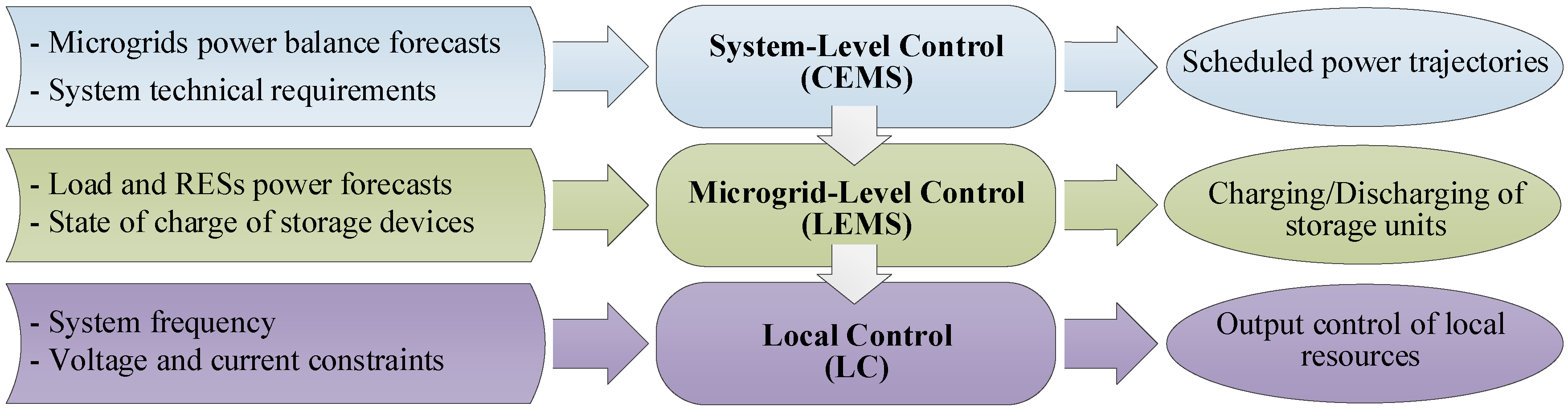
In this regard, a hierarchical EMS is developed to tackle complexities in the integrated operation management of interconnected RE-based MGs in this paper. MGs in a neighborhood area desire to keep the power exchange level of the MMG system with the main grid around a reference trajectory. Considering the hierarchical structure of MGs control [31], the proposed methodology includes three control levels. The central energy management system (CEMS) at the system-level, is responsible for coordinating the operation of MGs and determining day-ahead optimal trajectory for power transactions with the main grid considering system technical requirements. During the operation day, in a 60-min scheduling cycle, local EMSs (LEMSs) at the MG-level are responsible for managing the charging/discharging process of storage devices based on the power references received from CEMS. Two-stage stochastic programming with recourse variables is adopted to mitigate the uncertainty of non-controllable generators production including wind turbine (WT) and PVs as well as the variability of loads. Finally, local controllers (LCs) are designed to follow the provided set points through LEMS of each MG. To distribute any penalty cost resulted from real-time power deviation systematically and fairly, a new method based on the line flow sensitivity factors is proposed in which penalty cost is allocated by following the MGs contribution in the power deviation. The effectiveness of the proposed approach is verified by hardware-in-the-loop (HIL) simulation study.

The main contributions of this paper can be summarized as follows:

• Modeling integrated energy management of an MMG system in a hierarchical framework;
• Proposing an efficient control strategy using MPC and two-stage stochastic programming with recourse;
• Developing a novel methodology for cost allocation among MGs using the line flow sensitivity factors.

The rest of this paper is organized as follows. Problem formulation is presented in Section 2. Two-stage stochastic programming with recourse and stochastic MPC are represented in Section 3 and Section 4, respectively. The proposed cost allocation procedure is introduced in Section 5. Section 6 and Section 7 are related to simulation and experimental results, respectively. Finally, Section 8 concludes the paper.

2. Problem Formulation

Adopting the dynamical system approach, each subsystem i can be represented as a stack variable with associated inflows and outflows. The inflow is related to the net MG production including the aggregated power generation of WTs ($P_{WT,r}^i\left(t\right)$) and PV units ($P_{PV,r}^i\left(t\right)$) as well as the power consumption ($L_i\left(t\right)$) as represented below.

$$\begin{array}{c}I{F}_i\left(t\right)=\sum _{r=1}^{N_{WT}^i}{P}_{WT,r}^i\left(t\right)+\sum _{r=1}^{N_{PV}^i}{P}_{PV,r}^i\left(t\right)-L_i\left(t\right),\end{array}$$

(1)

In (1), $P_{WT,r}^i\left(t\right)$ and $P_{PV,r}^i\left(t\right)$ represent the output power of the rth renewable unit in the ith MG at hour t. Besides, $N_{WT}^i$ and $N_{PV}^i$ are related to the number of WTs and PVs in the ith MG, respectively. On the other hand, according to the following equation, the outflow of the ith MG is the total power that is transferred from it to the neighboring MGs and the main grid where $N_i$ is the set of the ith MG neighbors including the main grid.

$$\begin{array}{c}O{F}_i\left(t\right)=\sum _{j\in N_i}{P}_{ij}\left(t\right).\end{array}$$

(2)

Assume that $I{F}_i\left(t\right)$ represents the net power balance of the ith subsystem which could be forecasted based on the historical data during the scheduling horizon T. MGs provide the CEMS with the day-ahead predicted values of $I{F}_i\left(t\right)$ with 1-hour time resolutions. Utilizing this abstracted form of information, each MG is modeled through its net power balance from the CEMS point of view, disregarding further details and complexities. Afterward, system-wide power flow analyses are conducted by CEMS to specify the amount of power to be transferred through power lines considering voltage and frequency constraints as well as system losses. Thus, the system is expected to be in balance based on the day-ahead predicted values, which means $I{F}_i\left(t\right)=O{F}_i\left(t\right),i=1,...,M-1,t=1,...,T$. Here, M is the total number of subsystems including the main grid with the assumption that the highest index is assigned to the upstream network.

After deciding day-ahead scheduling, the entire MMG system will be represented to the main grid as an aggregated load or generation unit through its net energy content (see (3)).

$$\begin{array}{c}{I}_M\left(t\right)=\sum _{i=1}^{M-1}O{F}_i\left(t\right).\end{array}$$

(3)

Considering day-ahead power scheduling, IMGs are required to exchange power with the main grid according to the pre-specified trajectory of $I_M\left(t\right)$. However, the intrinsic uncertainty of RESs production and the variability of loads as well as the forecasting errors will result in uncertain behavior of MGs’ real-time power balance quantities. It is assumed that any real-time power deviation will be technically compensated by the main grid to guarantee the stability of the system. However, a large penalty cost will be imposed on the MGs. Consequently, MGs are required to devise operation strategies to compensate for the uncertainty locally at the MGs level. In this paper, to reduce the computational complexity, it is proposed that a local variable named power mismatch can be defined for the individual MGs as follows, for which the desired value is zero.

$$\begin{array}{c}{\delta }_{mis,i}\left(t\right)={\widehat{OF}}_i\left(t\right)-O{F}_i\left(t\right).\end{array}$$

(4)

In other words, it is desired that the realized outflow of each MG (${\widehat{OF}}_i\left(t\right)$) follows the estimated trajectory for the outflow of the MG ($O{F}_i\left(t\right)$). However, accounting for the inherent uncertainty of the MGs, this constraint cannot be fully guaranteed before the realization of the uncertain parameters. Thus, it is assumed that each MG is equipped with an energy storage system (ESS), which can be used as an appropriate tool to mitigate the uncertainty. The cost function of each MG is to minimize the operation cost of ESS unit as represented in the following.

$$min{c}_i\left|P_{b,i}\left(t\right)\right|.$$

(5)

In (5), $c_i\left(\frac{\$}{kW}\right)$ represents operational cost of the ESS in the ith MG and $P_{b,i}\left(t\right)$ is the amount of charging/discharging power, which is assumed to be positive/negative during charging/discharging intervals.

The LEMS of each MG is responsible to efficiently devise charging/discharging strategies of ESSs in the associated subsystem. Considering the uncertain nature of generation and demand parameters, LEMS tries to keep the possible power mismatch between realized and predicted trajectories of the MG outflow around zero while minimizing the ESS operational cost. Consequently, the control problem of each MG can be considered as a decentralized optimization problem with the following constraints in which (10) is a random constraint.

$$\begin{array}{c}s.t.SO{C}_i(t+1)=SO{C}_i\left(t\right)+\frac{P_{b,i}\left(t\right)}{E_{b,i}}\Delta ,\end{array}$$

(6)

$$\begin{array}{c}{P}_{b,i}^{min}\le P_{b,i}\left(t\right)\le P_{b,i}^{max},\end{array}$$

(7)

$$\begin{array}{c}SO{C}_i^{min}\le SO{C}_i\left(t\right)\le SO{C}_i^{max},\end{array}$$

(8)

$$\begin{array}{c}{\widehat{OF}}_i\left(t\right)=\sum _{r=1}^{N_{WT}^i}{\widehat{P}}_{WT,r}^i\left(t\right)+\sum _{r=1}^{N_{PV}^i}{\widehat{P}}_{PV,r}^i\left(t\right)-{\widehat{L}}_i\left(t\right)-P_{b,i}\left(t\right),\end{array}$$

(9)

$$\begin{array}{c}{\delta }_{mis,i}\left(t\right)=0.\end{array}$$

(10)

In (6), $SO{C}_i$ represents state of charge of the ESS in the ith MG and $E_{b,i}$ is its nominal capacity. Besides, $\Delta$ refers to the time length between two consecutive steps, which is assumed to be equal to 1h in this study. In (9), ${\widehat{P}}_{WT,r}^i\left(t\right)$, ${\widehat{P}}_{PV,r}^i\left(t\right)$, and ${\widehat{L}}_i\left(t\right)$ refer to the realized power values of the rth WT and PV units and the total power consumption in the ith MG at time slot t, respectively.

Taking into account the dynamical equation of the storage devices, successive time steps will be related to each other. Accounting for the system’s dynamics and accommodating the stochastic nature of the tracking constraint, a two-stage stochastic MPC approach is adopted to achieve the desired solution strategy. The optimal operating set points designed at this level are followed by the local controllers of each MG. Figure 1 illustrates the proposed hierarchical control structure along with the required input data and associated outputs of each control layer.

3. Two-Stage Stochastic Programming with Recourse

In the two-stage stochastic programming with recourse variables, decision variables include the first and the second-stage variables. The first-stage decision variables are determined before the realization of uncertainty while the second-stage variables are set after uncertain parameters are realized and considered as recourse variables (actions). Taking into account the second-stage variables for compensating any real-time infeasibility, the first-stage decision variables are determined with the allowance of constraint violation as a result of changing random parameters [32,33]. In other words, in this model, the constraints which include random parameters are modeled as soft constraints. To have a more quantitative point of view, consider the optimization problem illustrated in the following.

$$\begin{array}{c}min{C}^{T}x,\end{array}$$

(11)

$$\begin{array}{c}Ax=b,\end{array}$$

(12)

$$\begin{array}{c}Tx+H\mu =0,\end{array}$$

(13)

$$\begin{array}{c}x\in X.\end{array}$$

(14)

In (11)–(14), $x\in R^{n_1}$ represents the first-stage decision variables and $\mu \in R^r$ contains the uncertain parameters. In (12), A and b belong to the $R^{m_1\times n_1}$ and $R^{m_1}$, respectively. While the constraint represented in (12) is a deterministic constraint, the random constraint of (13) includes both deterministic and random parameters where $T\in R^{m_2\times n_1}$ and $H\in R^{m_2\times r}$ are coefficient matrices.

Since the only information about the uncertain parameters is their past behavior which could be incorporated to extract some statistical characteristics, these kinds of constraints could not be guaranteed to hold before the realization of random variables. In the two-stage stochastic programming, some slack variables ${\gamma }^{+}$ and ${\gamma }^{-}$ are introduced into the model as the second-stage decision variables as represented below.

$$\begin{array}{c}Tx+H\mu \le {\gamma }^{+},\end{array}$$

(15)

$$\begin{array}{c}-(Tx+H\mu )\le {\gamma }^{-}.\end{array}$$

(16)

In (15) and (16), ${\gamma }^{+}$ and ${\gamma }^{-}$ are slack variables, which represent corrective actions for compensating real-time infeasibilities. To deal with the violated random constraints, a second-stage or penalty function is included in the objective function. In general, the penalty function is considered in the form of $q^{+}{\gamma }^{+}+q^{-}{\gamma }^{-}$ in which $q^{+}$ and $q^{-}$ are penalty coefficients.

However, since the penalty function could only be evaluated after the realization of uncertain parameters, the second-stage cost could be replaced with an appropriate measure of risk. Thus, the first-stage decision variables should be selected in a process that encompasses possible realizations of $\mu$ represented by a finite set of scenarios. Considering the expected value for evaluating the probable penalty cost of different realizations of the uncertain variables and assuming finite discrete probability distribution for $\mu$, the two-stage stochastic optimization problem can be stated as follows.

$$\begin{array}{c}\underset{x,\gamma }{m}in{C}^{T}x+\sum _{j=1}^S{\pi }_j(q^{+}{\gamma }_j^{+}+q^{-}{\gamma }_j^{-}),\end{array}$$

(17)

$$\begin{array}{c}s.t.Ax=b,\end{array}$$

(18)

$$\begin{array}{c}Tx+H{\mu }_j\le {\gamma }_j^{+},\end{array}$$

(19)

$$\begin{array}{c}-(Tx+H{\mu }_j)\le {\gamma }_j^{-},\end{array}$$

(20)

$$\begin{array}{c}x\in X,{\gamma }_j^{+},{\gamma }_j^{-}\ge 0,j=1,...,S.\end{array}$$

(21)

In (17)–(21), S represents the number of scenarios and ${\pi }_j$ shows related discrete probability of the jth scenario. Thus, in a two-stage programming problem, the objective is to decide the first-stage decision variables such that the total cost including the operation cost and expected penalty cost resulted from real-time constraint violation is minimized. Although increasing the number of scenarios will result in improving quality of the solution, a long computational time might be required. Consequently, the solution quality should be traded against tractability of the problem.

4. Two-Stage Stochastic Model Predictive Control Formulation

In this section, the operation management problem of IMGs is formulated in the framework of two-stage stochastic MPC with recourse. In MPC, based on a dynamical model of the system under consideration, an optimal control sequence is derived over the desired control horizon. Intrinsic robust characteristics of MPC due to the rolling horizon strategy as well as its capability to account for operational and time-coupling constraints, make it a consistent solution strategy for power system applications.

Based on the two-stage stochastic approach that has been outlined in the previous section, the operation management problem of MGs can be represented as follows:

$$\begin{array}{c}\hfill \underset{\begin{array}{c}{P}_{b,i}(t,...,t+H_u-1),\\ {\gamma }_{i,j}^{+},{\gamma }_{i,j}^{-}(t,...,t+H_p-1)\end{array}}{min}\sum _{k=0}^{H_u-1}{c}_i{P}_{b,i}(t+k)+\\ \hfill \sum _{k=0}^{H_P-1}\sum _{j=1}^S{\pi }_{i,j}(q_i^{+}{\gamma }_{i,j}^{+}(t+k)+q_i^{-}{\gamma }_{i,j}^{-}(t+k)),\end{array}$$

(22)

$$\begin{array}{c}\hfill s.t.SO{C}_i(t+k+1)=SO{C}_i(t+k)+\frac{P_{b,i}(t+k)}{E_{b,i}}\Delta ,\end{array}$$

(23)

$$\begin{array}{c}\hfill P_{b,i}^{min}\le P_{b,i}(t+k)\le P_{b,i}^{max},\end{array}$$

(24)

$$\begin{array}{c}\hfill SO{C}_i^{min}\le SO{C}_i(t+k)\le SO{C}_i^{max},\end{array}$$

(25)

$$\begin{array}{c}\hfill {\delta }_{mis,i,j}(t+k)\le {\gamma }_{i,j}^{+}(t+k),\end{array}$$

(26)

$$\begin{array}{c}\hfill -{\delta }_{mis,i,j}(t+k)\le {\gamma }_{i,j}^{-}(t+k),\end{array}$$

(27)

$$\begin{array}{c}\hfill {\gamma }_{i,j}^{+}(t+k),{\gamma }_{i,j}^{-}(t+k)\ge 0,\\ \hfill k=0,...,H_p,j=1,...,S.\end{array}$$

(28)

In (22)–(28), $H_P$ and $H_u$ refer to the prediction and control horizons, respectively. In addition, ${\pi }_{i,j}$ represents the occurrence probability of the jth scenario in the ith MG and ${\gamma }_{i,j}^{-}(t+k)$ and ${\gamma }_{i,j}^{+}(t+k)$ are the recourse actions to take if the jth scenario occurs in the ith MG at time instant $t+k$ while staying in t. Furthermore, ${\delta }_{mis,i,j}(t+k)$ is the possible scenario of the uncertain parameter ${\delta }_{mis}$ at the time-step $t+k$ in the jth scenario and the ith MG.

At 60-min time intervals, the LEMS of each MG measures the level of stored energy in the battery and solves the optimization problem (22)–(28) to obtain the optimal control sequence $P_{b,i}(t,...,t+H_u-1)$ and recourse variables ${\gamma }_{i,j}(t,...,t+H_p-1)$. The first sample of the optimal control sequence is applied to the local controllers and the control and prediction horizons are shifted. Consequently, at each time step there are $H_u+2\times S\times H_p$ decision variables and $2\times (H_u+(2S+1)H_p)$ constraints for each MG.

5. Efficient Cost Allocation Strategy

In this paper, it is assumed that MGs in a neighborhood area desire to represent the whole MMG system as a predictable entity to the main grid. In other words, the final goal is to minimize the net value of unexpected power transactions with the main grid. According to (3), the net exchanged energy of the MMG network with the main grid is equal to the summation of the flow of lines that connect MGs to the main grid. It is assumed that the network of MGs will be penalized according to the real-time power deviation from the scheduled plan as represented in (29) where $PCost$ stands for the penalty cost and $\lambda$ represents the cost factor ($\frac{\$}{kWh}$) imposed to the MMG system for one kWh energy deviation.

$$PCost=({\widehat{I}}_M\left(t\right)-I_M\left(t\right))\lambda .$$

(29)

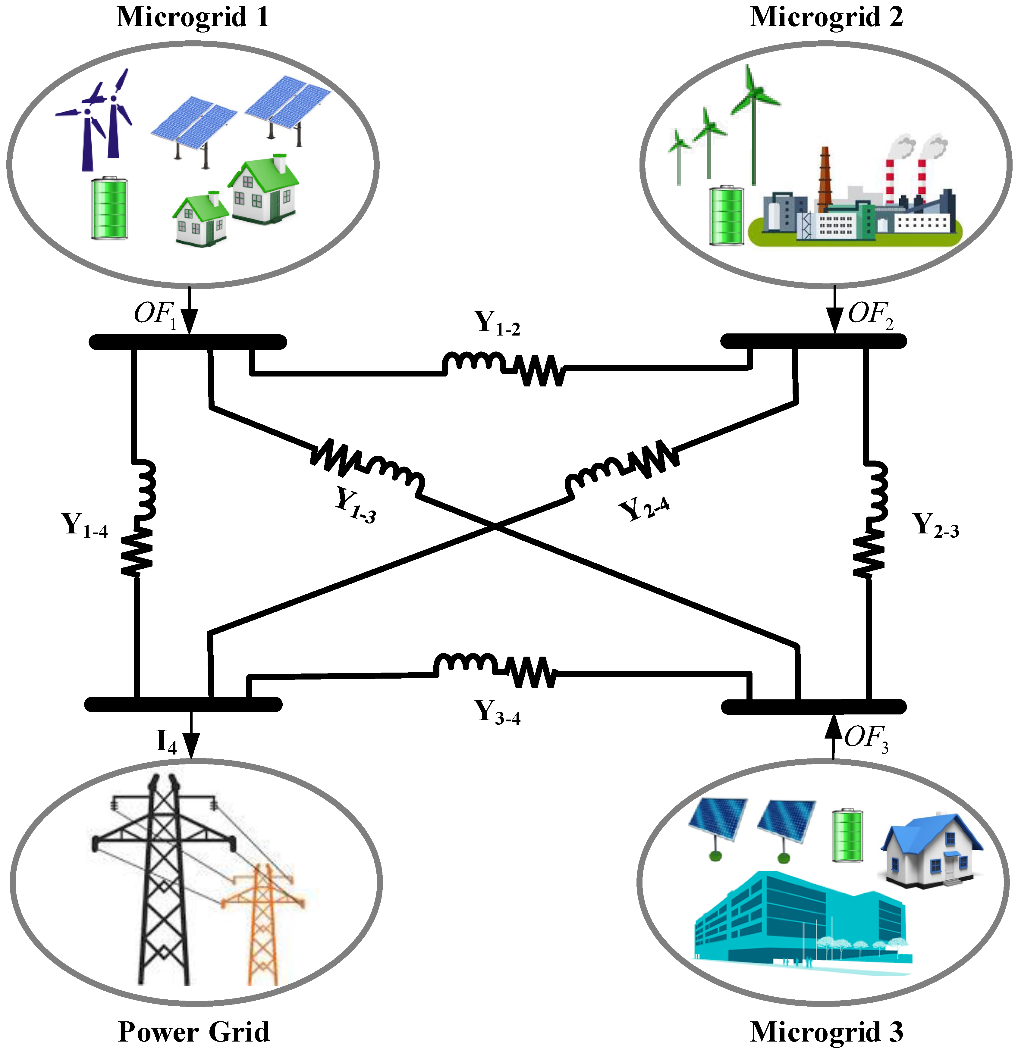
In this paper, it is proposed that the final penalty cost could be distributed among MGs ($\lambda ={\sum }_{i=1}^{M-1}{\lambda }_i$) by following their participation level. In other words, one should calculate the effect of power deviation in different MGs in the change of $I_M\left(t\right)$ from the reference value. Considering an exemplary system diagram for $M=4$ as represented in Figure 2, changes in $I_M\left(t\right)$ is equal to the summation of the line flow changes in different lines that connect the MGs to the main grid as shown below.

$$\Delta I_M\left(t\right)=\Delta f_{1-M}+\Delta f_{2-M}+...+\Delta f_{(M-1)-M}.$$

(30)

In (30), $\Delta f_{n-m}$ represents the change in power flow of the line $n-m$, which connects the nth bus to the mth bus. According to [34], it is assumed that any power changes $\Delta P_i$ at the ith bus of the system will be compensated through an exact opposite change in the reference bus, which is assumed to be the main grid in this study while the power generation in other buses remains fixed. Since power changes in the generation of different MGs do not have the same effect on the power flow of the intended line, the line flow sensitivity factors are used to measure different MGs effect and to share the penalty cost fairly.

Difference between the expected line power flow ($f_{n-m}\left(t\right)$) and the realized line power flow (${\widehat{f}}_{n-m}\left(t\right)$) can be represented as follows:

$$\Delta f_{n-m}\left(t\right)={\widehat{f}}_{n-m}\left(t\right)-f_{n-m}\left(t\right).$$

(31)

Considering the effects of power changes in different MGs on the line $n-m$ and defining ${\alpha }_{(n-m),i}$ as the sensitivity of line $n-m$ power flow to a change of $\Delta P_i$ in the ith MG, $\Delta f_{n-m}\left(t\right)$ could be written as below.

$$\Delta f_{n-m}\left(t\right)=\sum _{i=1}^{M-1}{\alpha }_{(n-m),i}\Delta P_i\left(t\right).$$

(32)

Utilizing (30), the change in power flow of the reference line concerning different MGs can be calculated as follows:

$$\Delta I_M\left(t\right)=\sum _{i=1}^{M-1}\Delta f_{M-i}\left(t\right),$$

(33)

$$\Delta I_M\left(t\right)=\sum _{i=1}^{M-1}{\alpha }_{(M-i),1}\Delta P_1\left(t\right)+...+\sum _{i=1}^{M-1}{\alpha }_{(M-i),M-1}\Delta P_{M-1}\left(t\right).$$

(34)

According to (35), the change in the flow of a line can be written using the phase angle change in the two buses n and m where the line is connected [34]. In (35), $x_{n-m}$ represents the line reactance. Moreover, using the linear power flow equations, the phase angles and power change of buses are related according to (36) where $\left[X\right]$ is derived from the admittance matrix [34].

$$\Delta f_{n-m}=\frac{1}{x_{n-m}}(\Delta {\theta }_n-\Delta {\theta }_m),$$

(35)

$$\Delta \theta =\left[X\right]\Delta P.$$

(36)

Hence, the line flow sensitivity factors are derived as follows:

$${\alpha }_{(n-m),i}=\frac{d{f}_{n-m}}{d{P}_i}=\frac{d}{d{P}_i}\left[\frac{1}{x_{n-m}}({\theta }_n-{\theta }_m)\right]=\frac{1}{x_{n-m}}(X_{n-i}-X_{m-i}).$$

(37)

It should be noted that if the lth bus is the reference bus, then $X_{l-i}=0$, $X_{i-l}=0$. Utilizing (34) and (37), the penalty cost coefficient of each MG can be considered as the normalized value of the line flow sensitivity factors.

$${\lambda }_i=s_i\lambda i=1,...,M-1,$$

(38)

$$s_i=\frac{{\sum }_{j=1}^{M-1}{\alpha }_{(M-j),i}}{{\sum }_{i=1}^{M-1}{\sum }_{j=1}^{M-1}{\alpha }_{(M-j),i}}.$$

(39)

6. Simulation Results

In this section, to evaluate the effectiveness of the proposed approach, simulation analyses are carried out in a test system. The model is established in MATLAB/Simulink. The nominal voltage and frequency of the system are set to $230\sqrt{2}V$ and $50Hz$, respectively. Matlab SimPower Systems is used to model the electrical system. The line impedance information is represented in

Table 1. Electrical system parameters.

Parameter	Symbol	Value
Frequency	f	50 Hz
Nominal Voltage	$V_{nom}$	$230\sqrt{2}$ V
Line Impedance 1,2	$Z_{1,2}$	$R_{1,2}=0.4\mathsf{\Omega },L_{1,2}=1mH$
Line Impedance 1,3	$Z_{1,3}$	$R_{1,3}=0.4\mathsf{\Omega },L_{1,3}=1mH$
Line Impedance 1,4	$Z_{1,4}$	$R_{1,4}=0.4\mathsf{\Omega },L_{1,4}=1mH$
Line Impedance 2,3	$Z_{2,3}$	$R_{2,3}=1\mathsf{\Omega },L_{2,3}=1.7mH$
Line Impedance 2,4	$Z_{2,4}$	$R_{2,4}=1\mathsf{\Omega },L_{2,4}=1.7mH$
Line Impedance 3,4	$Z_{3,4}$	$R_{3,4}=0.7\mathsf{\Omega },L_{3,4}=1.5mH$

.

The simulated system consists of three RE-based MGs that are equipped with battery-based ESSs in size of 350, 300, and 400 kWh, respectively. The initial level of SOC is set to $50\%$ of the nominal capacity, while the min and max SOC values are set to $20\%$ and $80\%$ of the battery nominal capacity, respectively. It is assumed that all MGs and the main grid are electrically connected and information can be exchanged among them to support bidirectional updates.

Table 2. Microgrids predicted aggregated load and RES generation [kW].

Time	MG1		MG2		MG3
	Load	RES	Load	RES	Load	RES
1	325.41	652.80	413.47	760.42	467.00	359.89
2	315.89	631.53	420.94	694.97	513.10	400.74
3	305.94	670.42	404.83	711.06	488.73	389.68
4	328.25	657.64	402.87	730.79	459.35	349.43
5	298.78	645.01	394.30	658.62	518.69	367.01
6	289.99	698.07	419.86	711.28	520.67	392.32
7	371.30	715.65	642.44	512.46	557.44	320.55
8	319.77	697.66	659.42	501.98	534.30	294.19
9	386.68	707.28	653.47	503.81	550.19	306.45
10	356.98	702.46	664.93	486.61	569.18	277.41
11	384.05	704.59	651.17	517.88	583.81	245.93
12	356.03	711.82	556.17	478.74	554.48	302.29
13	676.98	384.82	757.75	629.77	501.27	726.15
14	658.53	380.01	813.84	667.83	509.18	779.33
15	662.82	409.00	822.97	691.93	502.54	793.49
16	673.47	447.01	873.42	639.89	522.83	740.57
17	695.24	392.21	856.33	636.95	482.18	779.76
18	634.44	374.56	863.13	659.76	553.41	773.70
19	642.73	444.40	481.51	827.67	589.91	815.31
20	640.24	438.28	485.10	825.10	579.74	849.97
21	707.33	442.10	494.15	807.44	617.15	857.15
22	696.34	462.22	505.31	784.81	597.57	863.76
23	706.75	447.06	519.88	816.46	588.93	867.62
24	693.25	435.43	496.73	798.70	611.38	867.52

represents the predicted aggregated load profile of each MG during the optimization horizon and the forecast data for aggregated RESs production. To generate discrete random scenarios representing the uncertain nature of RESs production and consumer demand, Monte Carlo algorithm is used. Random scenarios are generated from normal distributions where the mean values are set to predicted data and standard deviations is assumed to 5% of the mean values for all MGs. Besides, $H_P=H_u=3$ h and $T=24$ h. The cost function is evaluated for a representative case where $c_i=0.2\frac{\$}{kW}$ and $\lambda =2\frac{\$}{kWh}$. 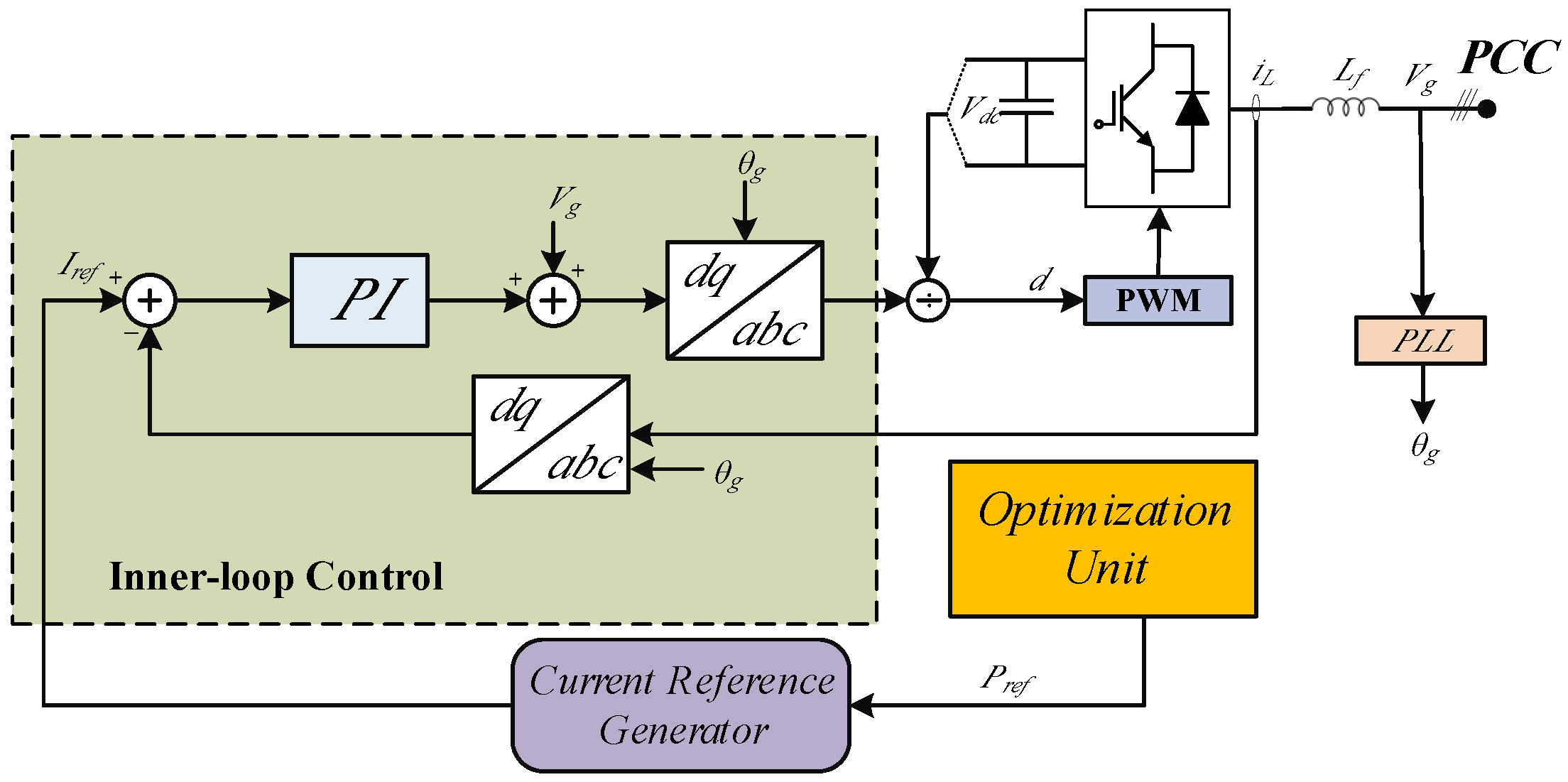Power flow analysis is conducted by CEMS using MATLAB SimPower System to specify the amount of power to be transferred through power lines. All electrical system requirements including voltage and frequency constraints, line capacity, and system losses are considered for deriving optimal power flows. A local PI controller as represented in Figure 3 is designed that controls each inverter output in current control mode. 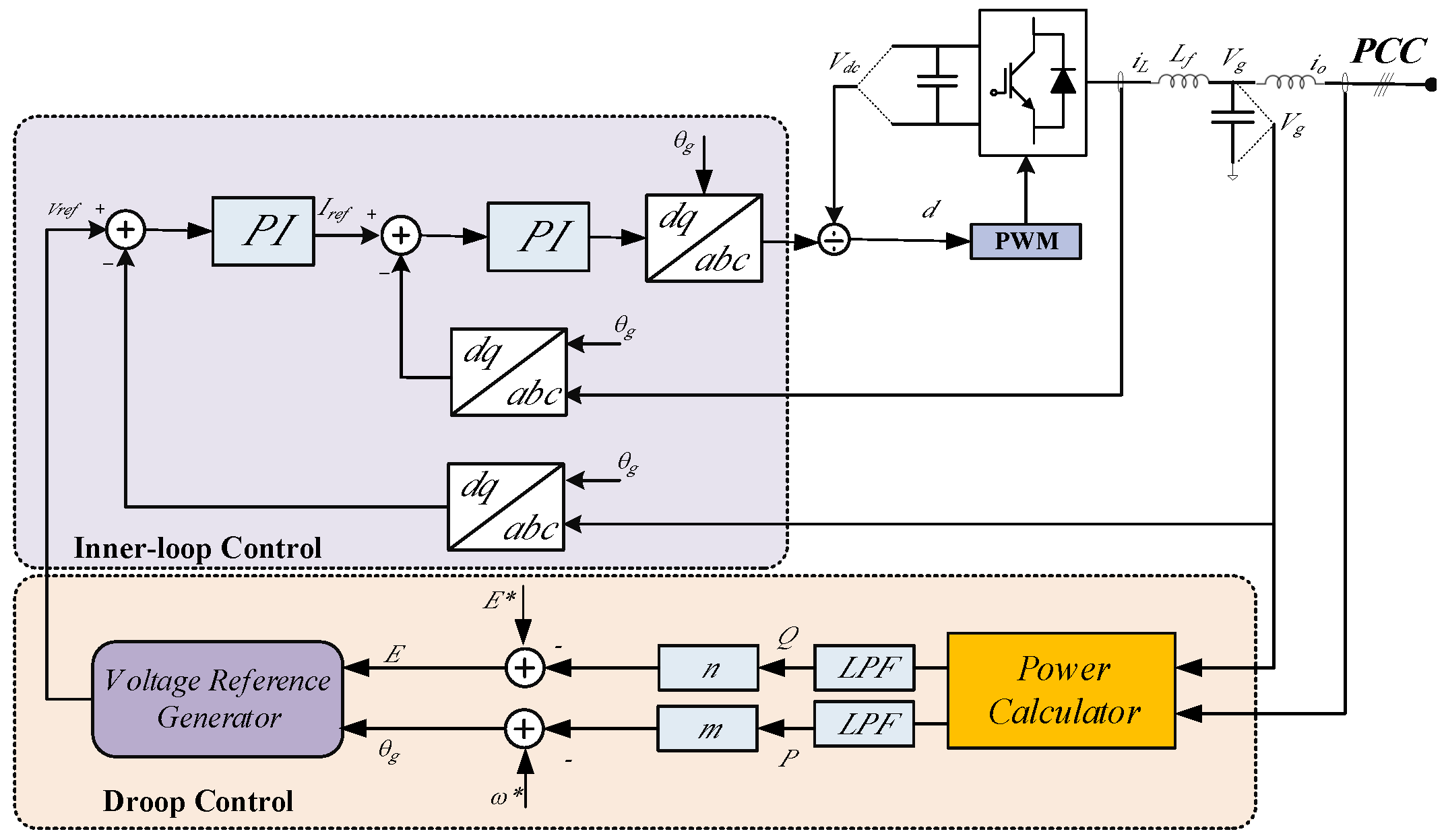The current proportional and integral terms are set to $K_{pI}=20$ and $K_{iI}=50\left[s^{-1}\right]$, respectively. For simulation purposes, the main grid is modeled using an inverter, which is controlled in voltage control mode as illustrated in Figure 4. For the experimental tests this part will be replaced by grid simulator. The current and voltage proportional and integral terms are set to $K_{pI}=15$, $K_{pV}=20$, $K_{iI}=50\left[s^{-1}\right]$, and $K_{iV}=50\left[s^{-1}\right]$, respectively. Using the proposed strategy for penalty cost allocation, the penalty coefficients have been calculated: $s_1=0.3184$, $s_2=0.3518$, $s_3=0.3299$.

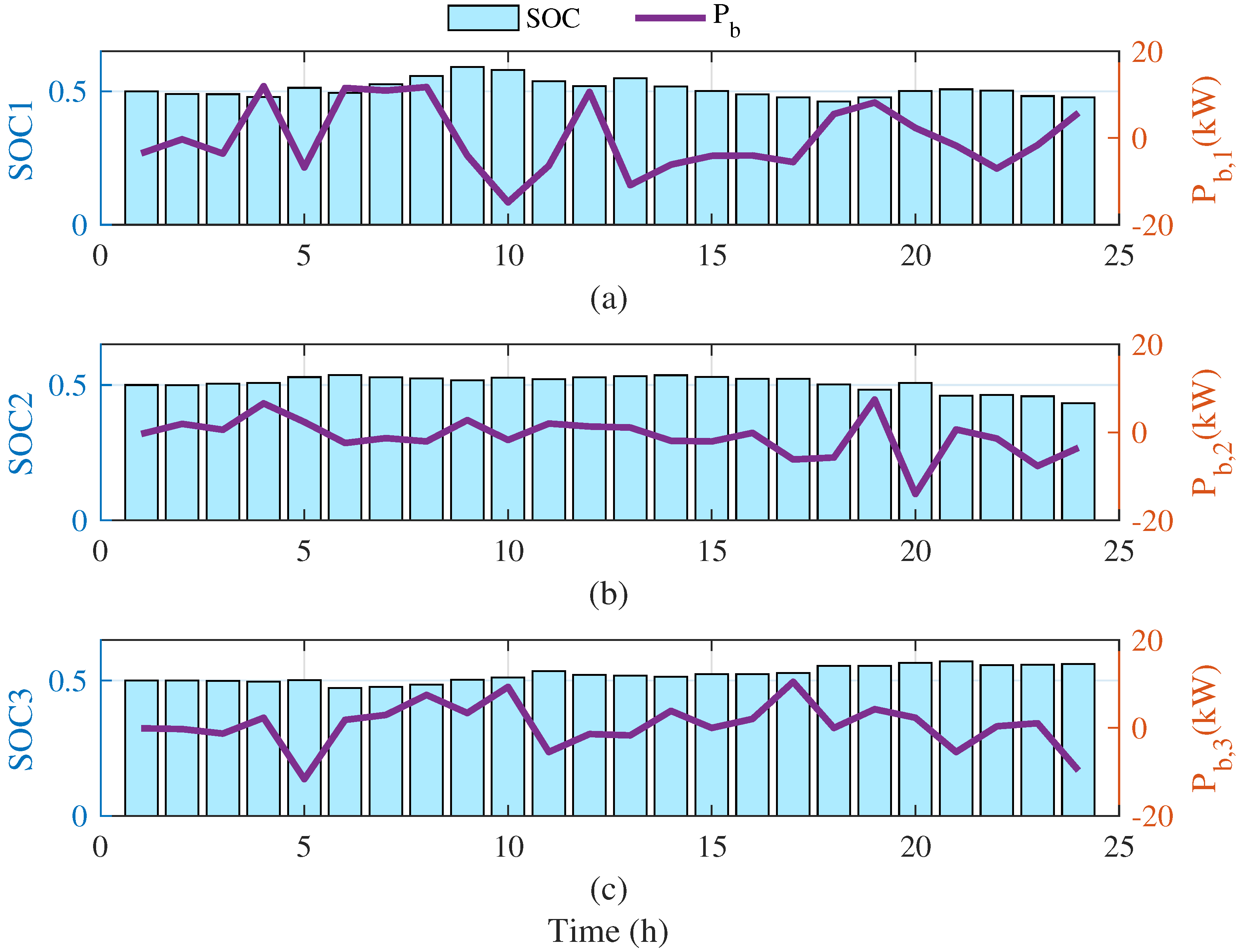
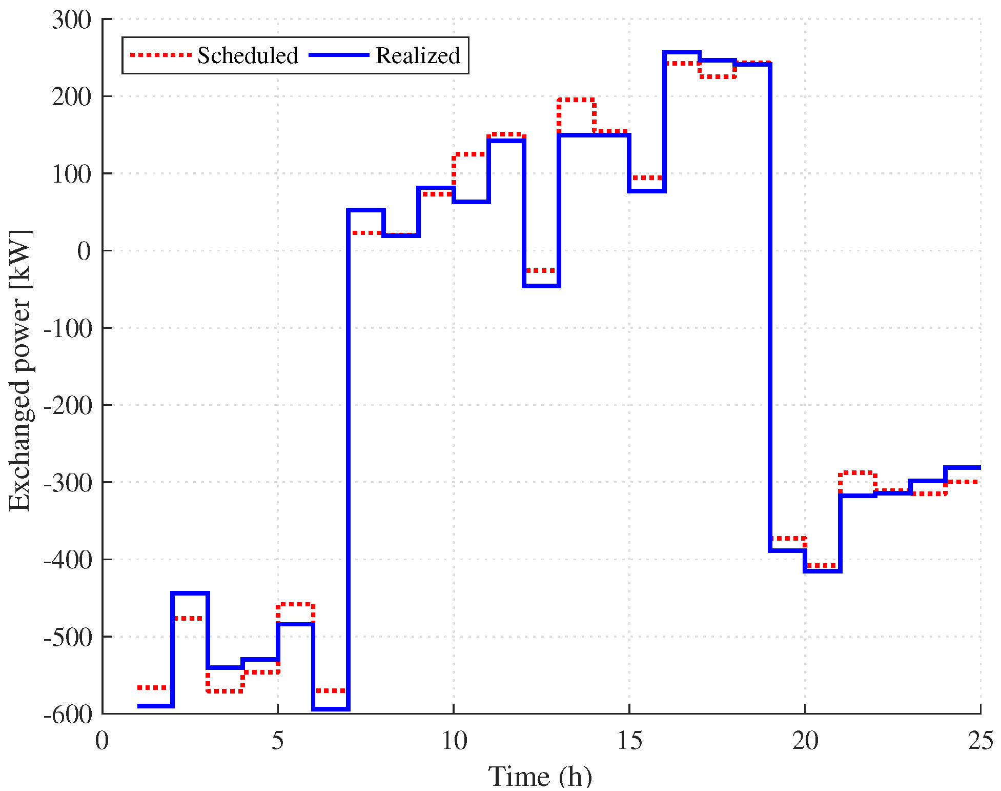
Figure 5 shows the daily ESSs scheduling for the MGs including the normalized SOC and charging/discharging power of the batteries, respectively. Scheduled and realized exchanged power between the MMG system and the utility is also plotted in Figure 6. As it can be noted, the proposed EMS has a good tracking performance in following the power reference trajectories.

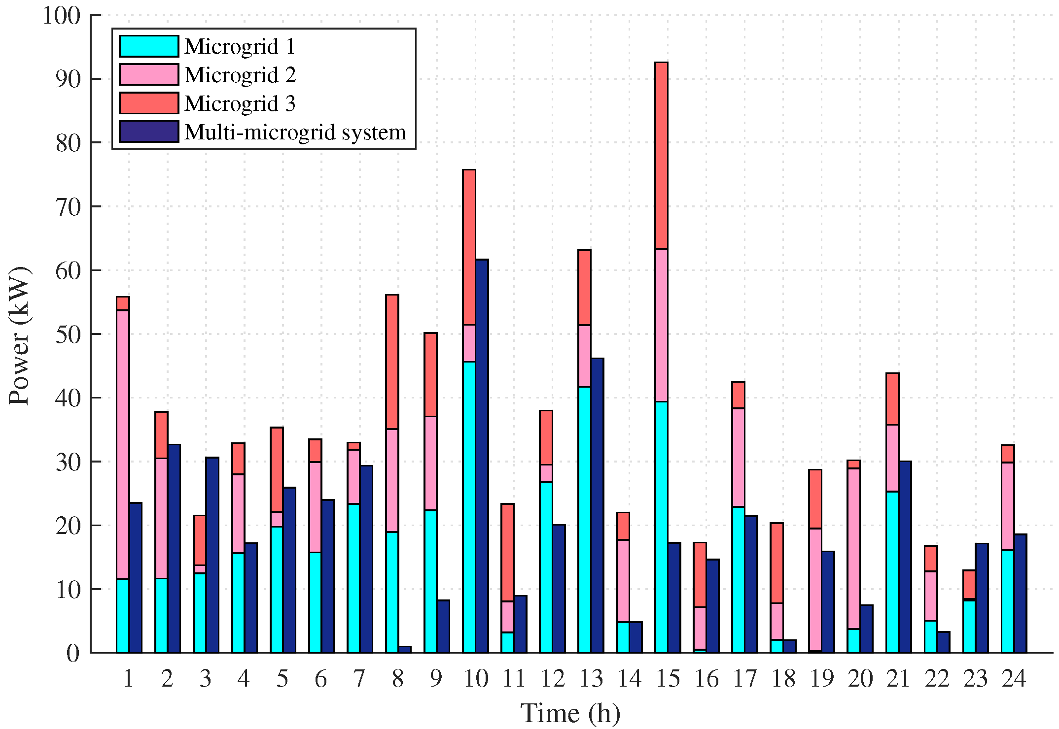
To evaluate the effects of the proposed approach on the unscheduled power exchange level of the MGs with the main grid, a single operation mode is assumed. In this mode, each MG is only allowed to exchange power with the main grid. As can be seen in Figure 7, the sum of power deviations of individual MGs is considerably higher than one related to the MMG system and a reduction of about 47% in the average unplanned daily power exchange of the IMGs with the main grid can be achieved. This can be considered as an advantage of the proposed strategy in reducing power system unscheduled power transactions. The penalty cost of MGs in both operating modes is tabulated in

Table 3. Penalty cost of MGs in different cases [$].

Operation Mode	MG 1	MG 2	MG 3	MMG
Single	794.01	589.82	448.17	1831.99
Coordinated	306.87	339.06	317.96	963.79

. According to the table, through coordinating the operation of MGs the penalty cost of each MG and the whole system will be reduced.

7. Experimental Results

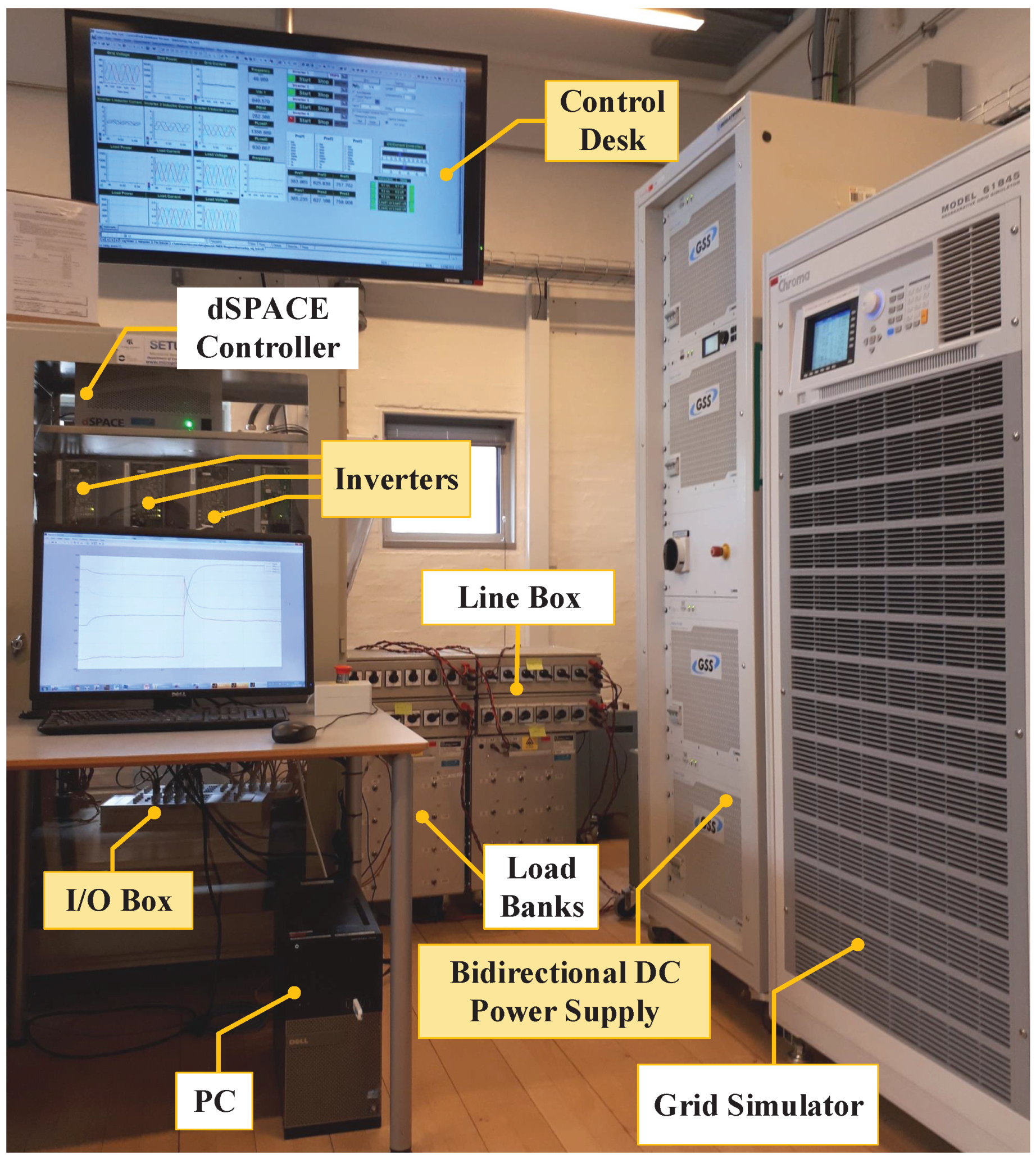
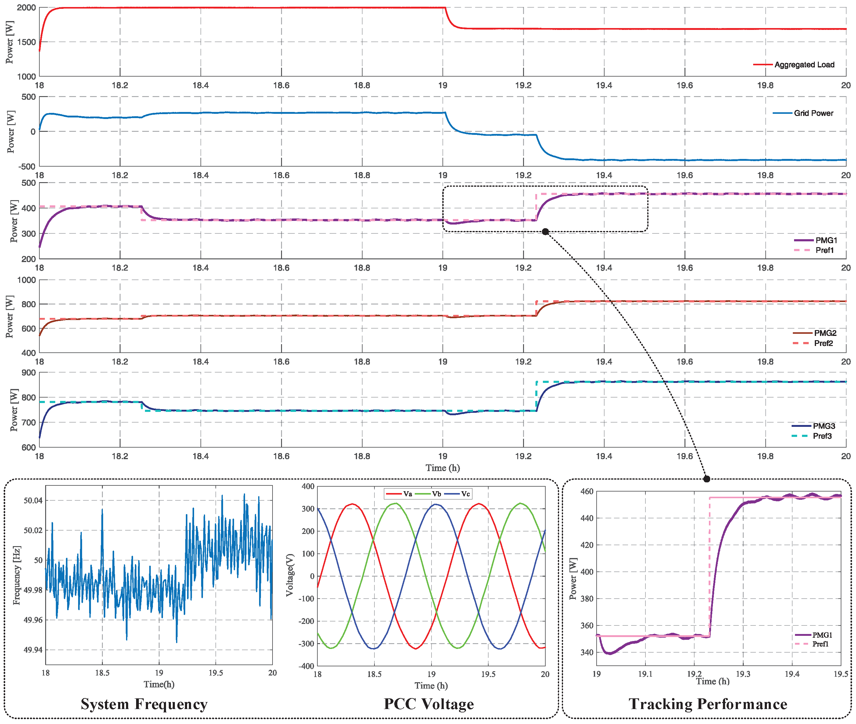
The test system has been implemented at the AC Microgrid Research Laboratory at Aalborg University as represented in Figure 8 [35]. A real-time platform (dSPACE 1006) is used for real-time simulation. As it can be noted, the setup includes three inverters (2.2 kW, $FC302$) fed through a stiff bidirectional DC source (0–800 VDC, 0–50 A, 64 kW), a regenerative grid simulator (45 kVA|330 V L-N) as well as line models, and load boxes. Due to the technical limitations, each MG is modeled by a single inverter. However, as the paper aims to show the capability of the MGs to follow reference trajectories, it will not raise any issue. It should be noted that generation/consumption profiles and the time slot have been scaled down such that 1000 W:1 W and 3600 s:20 s. Experimental tests are exemplary carried out in the time interval 18:00–20:00. Figure 9 represents the tracking performance of the local controllers. As can be seen, a good tracking performance has been achieved during the test interval. Moreover, taking into account the time scaling factor, the transient time of MGs is about 6s which approves the efficiency of the proposed approach in calculating and implementing optimal operation strategy and makes it applicable for real EMS. System frequency and voltage profile at PCC are also denoted in Figure 9. As can be seen in this figure, the system frequency has been kept within an acceptable range and a three-phase balanced output voltage regulation has been achieved.

8. Conclusions

In this paper, a novel control structure for integrated operation management of IMGs was proposed. The main goal was to represent the MMG system as a predictable entity to the main grid. To that end, a decentralized tracking control problem was designed for each MG and a two-stage stochastic MPC approach was adopted to derive the solution strategy. In the proposed scheme, any power deviation of the MMG system from the scheduled trajectory will be penalized. Considering the significant role of the MMG system in the next-generation power systems, designing systematic and fair cost allocation methodologies to motivate MGs participation in the cooperative energy management strategies is of vital importance. In this sense, a novel methodology for allocating the penalty cost among MGs using the line flow sensitivity factors was proposed. Analyzing other systematic cost allocation strategies is under study by the authors. Experimental results demonstrated the capabilities of the proposed approach to be incorporated as an efficient high-level controller in practical applications. According to the obtained results, adopting the proposed operation management strategy, a reduction of about 47% in the average unplanned daily power exchange of the IMGs with the main grid can be achieved. The reduction of unplanned power exchange with the main grid will result in a more predictable power exchange of the MMG system with the main grid as well as less penalty cost. From the viewpoint of the main grid, since the unscheduled power exchanges can be seen as disturbances, reducing it will result in lowering the complexity of power management of the main grid and more efficient reserve management strategies. Future studies of the authors are related to integrating learning-based methodologies in the EMS of MMG systems. Learning the behavior of MGs under different operating conditions will help develop more efficient EMSs in a less uncertain environment. Besides, recent advances in real-time monitoring and situational awareness of MGs will be deployed for early detection of system behavior changes from the predefined trajectories to activate the required responsive actions.