Article

Pipelined Dynamic Scheduling of Big Data Streams

by
Stavros Souravlas
1,2,* and
Sofia Anastasiadou
2
1
Department of Applied Informatics, School of Information Sciences, University of Macedonia Thessaloniki, 54616 Thessaloniki, Greece
2
Department of Early Childhood Education, Faculty of Education, University of Western Macedonia, 21, 53100 Florina, Greece
*
Author to whom correspondence should be addressed.
Appl. Sci. 2020, 10(14), 4796; https://doi.org/10.3390/app10144796
Submission received: 18 June 2020 / Revised: 4 July 2020 / Accepted: 5 July 2020 / Published: 13 July 2020
(This article belongs to the Section Computing and Artificial Intelligence)

Abstract

:
We are currently living in the big data era, in which it has become more necessary than ever to develop “smart” schedulers. It is common knowledge that the default Storm scheduler, as well as a large number of static schemes, has presented certain deficiencies. One of the most important of these deficiencies is the weakness in handling cases in which system changes occur. In such a scenario, some type of re-scheduling is necessary to keep the system working in the most efficient way. In this paper, we present a pipeline-based dynamic modular arithmetic-based scheduler (PMOD scheduler), which can be used to re-schedule the streams distributed among a set of nodes and their tasks, when the system parameters (number of tasks, executors or nodes) change. The PMOD scheduler organizes all the required operations in a pipeline scheme, thus reducing the overall processing time.

1. Introduction

Managing the large data volumes that arrive continuously can often exceed the capabilities of individual machines. Stream data processing requires continuous calculation without interruption and places high reliability requirements on resources. In this regard, it is important to develop efficient task-scheduling algorithms that reduce costs, improve resource utilization and increase the platform stability of Cloud services. Naturally, responsive schedules are required to keep pace with the transmission of massive data for large-scale tasks, and this aggravates the difficulty of the workflow scheduling problem [1,2]. An important challenge presents itself when the system parameters (especially the number of available nodes and executing tasks) need to change during runtime. This is a quite natural scenario, considering the fact that an application may require more resources from the Cloud when they are available or, in the reverse scenario, some resources (such as nodes) may become temporarily unavailable while an application is running.
Several data stream processing systems (DSPSs) that take advantage of the inherent characteristics of parallel and distributed computing, such as Apache Storm [3], Spark Streaming [4], Samza [5] and Flink [6], have specifically emerged to address the challenges of processing high-volume, real-time data. Specifically, the default Storm scheduler has become the point of reference for most researchers, who compare their proposed schemes against this simplistic scheduling algorithm. The main drawbacks of the Storm scheduler are as follows:
  • It does not offer optimality in terms of throughput;
  • It does not take into account the resource (memory, CPU, bandwidth) requirements/availability when scheduling;
  • It is unable to handle cases in which system changes incur.
In this work, we propose a pipelined modular arithmetic-based approach (the PMOD scheduler), which is based on the idea of each node receiving tuples for processing only from one other node at a time. The PMOD scheduler is proven to have some important advantages such as almost perfect load balancing, which is very important in today’s Cloud systems [7], minimized buffer requirements and higher throughput. The PMOD organizes all the required operations (tuple transfer, tuple processing and tuple packing, which will be discussed in Section 5) in a pipeline fashion, thus decreasing the overall execution time compared to other known schemes, as the experimental results show.
The remainder of this work is organized as follows: Section 2 briefly summarizes some important dynamic scheduling approaches and describes the methodology on which their scheduling strategy is based. Section 3 gives a brief motivating example so that the reader can better understand the motivation behind a dynamic strategy. Section 4 describes the necessary mathematical background. Section 5 presents the PMOD scheduler. In Section 6, we present our comparison results, and Section 7 concludes the paper and offers perspectives for future work.

2. Related Work

In this paragraph, we describe some of the most important dynamic strategies found in the literature. Before this, we make a short reference to the static big data scheduling strategies. The static strategies work offline and try to assign the tasks to the most suitable nodes in order to minimize the communication latencies between tasks that need to co-operate during the execution of an application. A number of static strategies are topology-aware, such as those listed in [8,9,10], while others are based on resource handling (resource-aware), such as those in [11,12] or [13]. Finally, other recent works employ the idea of linear programming; for example, this is evident in [14,15,16,17].
In this paragraph, we focus on dynamic big-data scheduling strategies. The dynamic strategies monitor performance parameters during runtime and update tasks’ placement. Decisions are made online. However, issues such as re-balancing can be proven to be highly time-consuming; e.g., ≈200 s in Storm [11] (recent works have tried to develop techniques for rapid re-balancing [18,19]). Moreover, several existing works employ the CPU without considering memory constraints [18,20], and this can lead to memory overflow.
A dynamic scheme should be able to handle system changes (number of tasks or nodes) that occur after monitoring and during runtime. Additionally, it should be able to adopt data parallelism and scale out the number of parallel instances for an operator that is overloaded [11]. Many dynamic works employ task migrations, which are required to reduce resource utilization imbalances between nodes. This is a costly procedure, and it is not employed in our work. Below, we briefly describe some of the most important works presented in the literature.
Aniello et al. [8] developed a dynamic online scheduler that produced assignments that reduced the inter-node and inter-slot traffic on the basis of the communication patterns among executors observed at runtime. The goal of an online scheduler is to allocate executors to nodes in order to impose limitations on the number of workers each topology has to run on, the number of slots available for each worker node and the computational power available on each node. There are two phases in this implementation: in the first phase, the pairs of communicating executors of each topology are put in descending order based on the rate of exchanged tuples. For each of these pairs, if both the executors have not been assigned yet, they are assigned to the least loaded worker. Otherwise, to choose the best worker, a set is generated by putting the least loaded worker together with the workers where either executor of the pair is assigned and the assignment decision is based on the criterion of the lowest inter-worker traffic. The latency of processing an event is below 20–30% and the inter-node traffic below 20% with respect to the default Storm scheduler in both tested topologies.
Fu et al. [18] designed and implemented the DRS (dynamic resource scheduler). Their algorithm takes into account the number of operators in an application and the maximum number of available processors that can be allocated to them and tries to find an optimal assignment of processors that results in the minimum expected total sojourn time. They estimated the total sojourn time of an input by modeling the system as an open queuing network (OQN). The performance model is built based on a combination of one of Erlang’s models and the Jackson network. The system monitors the actual total sojourn time and checks if the performance falls or whether the system can fulfill the constraint with fewer resources, rescheduling if necessary. It repeatedly adds one processor to the operator with the maximum marginal benefit, until the estimated total sojourn time is no larger than a real-time constraint parameter. DRS uses Storm’s streaming processing logic and demonstrates robust performance, suggesting the best resource allocation configuration, even when the underlying conditions of the queuing theory that it uses are not fully satisfied. In general, the overheads of DRS are less than milliseconds in most of the cases tested, resulting in a small impact on the system’s latency.
Meng-Meng et al. [21] proposed a dynamic task scheduling approach that considers links between tasks and reduces traffic between nodes by assigning tasks that communicate with each other to the same node or adjacent nodes. The topology is obtained by recording the workload of nodes and communication traffic through switches a priori. They used a matrix model to describe the real-time task scheduling problem. Their processing procedure tries to reduce traffic between nodes through switches, cut off bandwidth pressure and balance the workload of nodes by selecting the appropriate host node when a trigger (either node-driven or task-driven) occurs. They evaluated their algorithm by deploying their own stream processing platform and compared their solution with algorithms built in Storm and S4 using the load balance and communication traffic through switches as indicators. As the number of jobs running in these platforms increased, the load balance improved. Moreover, less stream data flowing through switches were detected, and this traffic was reduced, relieving the bandwidth pressure of the cluster. This scheduler is based on similar ideas to that presented in our work and will be used for comparisons, as will be explained in the experimental results section.
T-Storm, developed by Xu et al. [20], is another attempt to minimize inter-node and inter-process traffic. Workload and traffic load information are collected at runtime by load monitors to estimate the future load using a machine learning prediction method. A schedule generator periodically reads the above information from the database, sorts the executors in descending order of their traffic load and assigns executors to slots. Executors from one topology are assigned in the same slot to reduce inter-process traffic. The total executor workload should not exceed the workers’ capacity, and the number of executors per slot is calculated with the help of a control parameter. T-Storm consolidates workers and worker nodes to achieve better performance with even fewer worker nodes, enables the hot-swapping of scheduling algorithms and adjusts scheduling parameters on the fly. T-Storm’s evaluation shows that it can achieve an over 84% and 27% speed-up of average processing time on lightly and heavily loaded topologies, respectively, with 30% fewer worker nodes compared to Storm.
System overload is also a matter of interest for Liu et al. [22]. They proposed a dynamic assignment scheduling (DAS) algorithm for big data stream processing in mobile Internet services. The authors generated a structure called the stream query graph (SQG) based on the operators and the relations between the corresponding input and output. SQG is a direct acyclic graph, and an edge between two nodes represents a task queue. The edge weight is the number of tasks in the queue. The minimum-weight edge is selected to send tuples, and a buffer list is set to store some tuples before the next scheduling. The scheduling strategy of DAS is updated continuously by every logic machine separately. By splitting the general scheduling problem into a common sub-problem for every operator, the overhead is reduced and accuracy is improved.
Generally, elasticity is a matter of crucial importance in online environments, as the input rate can vary drastically in streaming applications, and operators’ replication degrees need to be configured to maintain system performance. Unfortunately, most of the available solutions require users to manually tune the number of replicas per operator, but users usually have limited knowledge about the runtime behavior of the system. Several approaches (e.g., [19,23]) have attempted to deal with replication runtime decisions in stream processing.
Dynamic techniques, while advantageous, can lead to local optima for individual tasks without regard to the global efficiency of the dataflow. This introduces latency and cost overheads. The application’s reconfiguration and re-balancing, quite often consisting of migrations, may also be time-consuming. In our work, we eliminate local optima for tasks and we present a dynamic scheme with a perfect load balance between task. Moreover, task migration—a very costly procedure—is completely avoided. The buffering memory required is reduced because of the “one-to-one” communication between the system’s nodes imposed by our work.

3. A Motivating Example

Let us consider a cluster of N = 6 nodes and an application topology such as the one in Figure 1, in which the interconnection between the components is shown. In this figure, there are four bolts and one spout, each of which have t = 4 threads. Each thread executes one task, so we can refer to tasks and threads interchangeably hereafter.
Our offline (static) strategy [1] uses a set of matrix transformation based on linear algebra theory that aims (1) to produce a series of communication steps such that each node communicates to exactly one other node at a time, and (2) to place the tasks in the most suitable (in terms of distance) nodes, so that their communication (as defined by the application topology) is implemented with the minimum communication latency. In short, our strategy initially defines the initial matrix, M i n i t , as a table that stores the tasks assigned to each node by the default round-robin Storm scheduler. This table can have two forms: in the first form, the tasks are indicated as letters, and in the second, they have been replaced by numbers.
M i n i t = N 0 N 1 N 2 N 3 N 4 N 5 Q R S T A B C D E F G H I J K L M N O P Ω Ω Ω Ω N 0 N 1 N 2 N 3 N 4 N 5 0 1 2 3 4 5 6 7 8 9 10 11 12 13 14 15 16 17 18 19
The tasks indicated by Ω are added by our model as “dummies” and are used to avoid empty values in M i n i t . In the numbered representation, the dummy tasks are circled. A dummy task plays no role in the actual processing. The scheduler performs a series of well-defined matrix transformations and uses a refinement phase to produce the final matrix M f i n . The refinement phase is used to allocate the tasks to the proper nodes, meaning that intercommunication latencies caused by the communication between tasks are reduced. Each row of this matrix indicates a communication step between the node labeled at the top of each column and the node index found in the specific row. For the example of Figure 1 the corresponding M f i n is
M f i n = N 0 N 1 N 2 N 3 N 4 N 5 0 1 2 5 3 4 1 0 5 2 4 3 3 4 0 1 2 5 4 3 1 0 5 2
and the communications defined by the first row are as follows: node 0 transfers tuples to node 0 (internal communication between the tasks residing in node 0), node 1 to node 1 (internal communication between the tasks residing in node 1), node 2 to node 2 (internal communication between the tasks residing in node 2), node 3 to node 5, node 4 to node 3 and node 5 to node 4. Internal task communications are preferred whenever possible, as they add no extra communication latencies.
Moreover, M f i n can be used to define the task allocations in each node. In this example, the equivalent task allocation matrix is
M f i n = N 0 N 1 N 2 N 3 N 4 N 5 Q A E Ω I M B R Ω F N J K O S C G Ω P L D T Ω H
which indicates that, for the specified application topology, the communication latencies are reduced by placing tasks Q,B,K and P to node N 0 , tasks A,R,O and L to node N 1 , etc.
Generally, the static approach does its best to find an optimal solution for a task allocation and scheduling problem. Specifically, the following tasks are addressed:
  • It reduces the buffering space required by each task, and the system’s throughput therefore increases (most of the tuples are processed as soon as they arrive at the processing node);
  • Load balancing is achieved (each node receives from only one node at each communication step, and thus lower communication latencies are achieved (no links are overloaded—instead, all links are equally loaded); and
  • The scheduling procedure has a log complexity.
However, there are cases in which the replication factor F (that is, the number of tasks run at each node) needs to increase by a percentage (for example, a 25% increase in the number of tasks per node will produce a problem with N = 6 and r = 5 ). In a different scenario, the number of nodes may need to change if a node crashes or if more nodes should be added to accommodate an application’s resource needs. In such scenarios, the scheduler has to make a fast online decision for re-allocating the tasks and re-scheduling them among the system’s nodes, meaning that the throughput increases and the overall latencies are reduced. In this paper, we propose a fast pipelined scheme that can be efficiently used for such dynamic scenarios. This scheme is described in Section 5; before this, we need to present its mathematical background.

4. Mathematical Background

In this paragraph, we present the mathematical notations required to implement the PMOD scheduler. The main idea behind what follows is not to re-allocate the tasks (this is not an efficient solution to follow as the program runs), but instead to organize all the communications in “homogeneous” groups in terms of communicating pairs, which will be used to achieve a schedule with reduced memory consumption and thus a higher achievable throughput and balanced load among all the nodes.
First, let us define an equation that describes the round-robin placement of r consecutive tasks into a set of nodes.
n = i / t mod N ,
where N is the number of nodes in the initial distribution, n is the node where task i is placed and t is the number of tasks. From Equation (2), for some integer L, we obtain
i / t = L N + n .
Now, if we set an integer x such that x = i mod t , 0 x < t , Equation (3) becomes
i = ( L N + n ) t + x
Equation (4) describes the initial task distribution. We use R ( i , n , L , x ) to symbolize this distribution. In a similar manner, we can derive an equation that describes the new distribution, according to the system changes. Assume that the number of nodes changes from N to Q; thus, Q is the number of nodes in the new distribution, q is the node where task j will be placed and s is the new number of tasks. Thus, we obtain
j = ( M Q + q ) s + y
where the integers M , y are defined in a similar manner to L and x in Equation (4). For y, we have 0 y < s . We use R ( j , q , M , y ) to symbolize a distribution that would occur in the case of the system changes described before. However, as stated at the beginning of this section, our aim is not to perform a task redistribution but to define sets of homogeneous communications that will rapidly produce an efficient communication schedule with reduced latencies. The idea is to equate the two distributions defined in Equations (4) and (5) and generate a linear Diophantine equation as follows:
R = R ( L N + n ) t + x = ( M Q + q ) s + y
 or
n t q s + ( x y ) = M Q s L N t
Such linear Diophantine equations are solved using the extended Eucidean algorithm in logarithmic time, which is perfectly suitable for our scheduler.
Now, we set G = g c d ( N t , Q s ) , making L N t M Q s a multiple of g. This means that there is an integer λ , such that L N t M Q s = λ g . If we also set z = x y , then (7) is rewritten as
λ g z = n t q s
From modular arithmetic, we are aware that, for linear Diophantine equations, a pair of processors ( p , q ) belongs to a communication class k if
( p t q s ) m o d g = k
Proposition 1 will make use of the definition of a class and Equation (7) to show the homogeneity of the processor pairs found in each class.  
Proposition 1.
All processor pairs that belong to a class are proven to be homogeneous in terms of the number of solutions that they produce for Equation (8).
Proof. 
We divide both parts of Equation (8) with g to obtain
( λ g z ) mod g = ( n t q s ) mod g
( λ g mod g ) ( z mod g ) = ( n t q s ) mod g
( 0 z ) mod g = ( n t q s ) mod g
z mod g = ( n t q s ) mod g .
Since z = x y , it is obvious that z = y x . Therefore, we derive the equation
( y x ) mod g = ( n t q s ) mod g o r ( y x ) m o d g = k
Equation (10) states that for every class k (and thus for its members—a set of communicating pairs), there is a constant number of combinations of x and y values, which we name c (recall that x and y are limited by t and s respectively), that produce k when we get their modulo to g. This proves Proposition 1. □
The main characteristics of classes [24,25,26] are summarized as follows:
  • The maximum number of classes that exist in a redistribution problem is g;
  • There may be two or more classes with the same value of c. This means that our communication schedule, which requires each node to send or receive tuples only from one node at a time, can freely mix elements from two or more such classes, which can also be considered homogeneous between them.
We now illustrate the ideas described in this paragraph with an example. Assume that, initially, we have N = 6 nodes with t = 4 tasks per node, and based on system monitoring, the replication factor F increases by 25%, necessitating the use of s = 5 tasks per node, while the number of nodes remains at six; that is, Q = 6 . We also have g = 6 . Then, Table 1, shows the communicating pairs that belong to each of the six classes. These pairs have been computed using Equation (9). Furthermore, from Equation (10), we have computed the c values for each class. The table that contains all this information is named the class Ttble (CT).
Note that classes 0 and 1 have the same c values. Moreover, we cannot rely separately on these classes to produce a communication schedule in which each node receives tuples from only one node, as there are communicating pairs with the same receiving node index; for example, ( 0 , 0 ) and ( 3 , 0 ) in class 0 or ( 0 , 1 ) and ( 3 , 1 ) in class 1. Similarly, the other four classes can be considered homogeneous with c = 3 . The next subsection will show how we use the classes to produce a pipelined scheduling scheme.

5. The PMOD Scheduler

The PMOD scheduler aims at dividing the overall tuple transmission into a set of communication steps, without re-positioning the tasks, so that the following characteristics are achieved.
1.
Each node receives tuples from only one other node. In other words, each node’s tasks receive tuples previously processed by the tasks of only one other node. The communicating tasks are defined by the application’s topology.
2.
Load balancing is achieved.
3.
The overall communication schedule is simple and fast, as it has to be implemented during runtime.
In the big data literature, the latency of communication between two nodes is generally defined by their index difference. For two nodes n i and n j , the communication latency increases as the difference | i j | becomes larger. In our example, if the tasks from node 5 need to send tuples to the tasks of node 0 or vice versa, we have the maximum possible latency of = | 5 0 | or = | 0 5 | = 5 time units. In our context, we use the term “time units” as a unit that measures the inter-node communication latencies. To organize the overall communication in a pipeline fashion, we first need to transform the class table (CT) into a table that defines the communication steps between different nodes. This is described in the following subsection, along with the theoretical approach of the communication cost.

5.1. Transforming the Class Table into a Scheduling Matrix

This transformation requires two steps.   
Step 1: Transform CT to a Single Index Matrix   
The first step transforms the CT to a single-index matrix ( S I M ). Each row of S I M describes a communication step based entirely on a single class. The communicating pairs of each class k reside in row k of the CT. We simply pick each communicating node pair ( n , q ) found in row k and place the value of q in column n of S I M . In our example, the CT will be transformed into the following S I M  matrix.
S I M = Communicating Step N 0 N 1 N 2 N 3 N 4 N 5 0 0 2 4 0 2 4 1 1 3 5 1 3 5 2 2 4 0 2 4 0 3 3 5 1 3 5 1 4 4 0 2 4 0 2 5 5 1 3 5 1 3
Step 2: Mix Class Elements to Define Communicating Steps  
Our scheduler requires that each communicating step requires Q communications. If each class includes α communications towards different destinations, we have to mix elements between Q / α homogeneous classes, α 2 . To mix class elements, we simply interchange α elements of homogeneous classes that reside in corresponding columns. In our example, α = 3 ; thus, we interchange three elements in columns N 3 N 5 of the homogeneous classes 0; 1, 2 and 3; and 4 and 5. This will produce the following scheduling matrix, ( S M ) :
S M = Communicating Step N 0 N 1 N 2 N 3 N 4 N 5 Communication Cost 0 0 2 4 1 3 5 2 1 1 3 5 0 2 4 3 2 2 4 0 3 5 1 4 3 3 5 1 2 4 0 5 4 4 0 2 5 1 3 4 5 5 1 3 4 0 2 5 23
The communication cost for each step is computed based on the maximum cost, max , found between the the communicating pairs. For example, in step 0, there is a communication between nodes 2 and 4 and between nodes 3 and 1. Thus, m a x = | 2 4 | = | 3 1 | = 2 . The remaining values are | 0 0 | = 0 , | 1 2 | = 1 , | 4 3 | = 1 and | 5 5 | = 0 (internal communication between tasks residing in node 5). Since all the communications start simultaneously, the latency of this step is dictated by max , so it equals 2. Similarly, we obtain all the costs for the other communication steps. Thus, the total communication cost for all the steps is the sum of the communication costs of the six communication steps, which is 23. Our third scheduling step aims to reduce this cost. The following proposition gives the theoretical approximation of the communication costs that exist within the S M .
Proposition 2.
The total cost of the communications, C S M , which are defined in the S M can be approximated by the following equation:
C S M = 2 ( Q 1 ) + 2 ( Q 2 ) + χ 1 ( Q 3 ) + χ 2 ( Q 4 ) + + χ ν ( Q 1 )
Proof. 
By mixing class elements (Step 2), we guarantee that all the communications are performed between different source and target nodes (see the S M matrix). We know that, in a set of Q 2 communications, the latency values q , q [ 0 , , Q 1 ] , and the number of communicating pairs that are characterized by q are as shown in Table 2:
For example, with  Q = 6 , there are two pairs with a cost of Q 1 = 5 ((5,0) and (0,5)) and six pairs with a cost of 0 (internal node communications; (0,0), (1,1), (2,2), (3,3), (4,4), and (5,5)). Additionally, there are 10 pairs with a cost of 1, eight pairs with a cost of 2, six pairs with a cost of 3 and four pairs with a cost of 4. Because of the way the S M is generated (different source and target indices per communication step), these pairs are, on average, equally distributed in the initial scheduling matrix. Specifically, each row of the S M has α elements from Q / α classes. The average latency is computed as follows: there are two node pairs with a maximum latency of Q 1 . Without loss of generality, we can assume that they are distributed in two rows of S M , producing a total latency of 2 ( Q 1 ) time units. These two pairs determine the overall latency of the communication steps defined in these rows, as they have the maximum latency. Similarly, the four elements with a cost of Q 2 are, on average, distributed in four (provided that Q 4 ) rows, and we determine the cost of four halves out of these four rows (in the average case, the latencies of half of these pairs are “absorbed” by the maximum latencies of Q 1 ; in other words, two of the pairs with a cost of Q 2 are in the same row as the pairs with a maximum cost of Q 1 ). Thus, we have an added latency from these steps equal to 2 ( Q 2 ) . There remain Q 4 rows to be examined. Continuing in this manner, the six elements with a cost of Q 3 are, on average, distributed in six rows (provided that Q 6 ) and we determine the latencies of 6 2 = 3 (provided that Q 4 3 ; otherwise, they determine the latencies of < 3 rows) out of these six rows (in the average case, the latencies of half of these pairs are “absorbed” by the larger latencies of Q 1 and Q 2 ; in other words, three of the pairs with a cost of Q 3 are in the same row as the pairs with larger costs of Q 1 and Q 2 ). Working similarly, we find that, on average, the total latency of the steps defined by the S M can be computed by Equation (11). □
Let us return to our example to see how Equation (11) applies:
C S M = 2 ( Q 1 ) + 2 ( Q 2 ) + χ 1 ( Q 3 ) + χ 2 ( Q 4 ) + + χ ν ( Q 1 ) = 2 × 5 + 2 × 4 + 1 × 3 + 1 × 2 = 23
where χ 1 = χ 2 = 1 .   
The next subsection describes how the S M will be used to implement the pipelined scheduling.

5.2. Pipelined Scheduling

Our pipelined approach divides the overall scheduling into three stages: (a) the transferring stage, (b) processing stage and (c) packing stage. The transferring stage is the stage at which data streams are forwarded according to the communicating steps defined by the S M . The maximum communication cost step is u and the remaining costs are < u . The transferring stage employs all the hardware necessary to forward the streams among the system’s nodes. The processing stage is the stage at which the streams are processed by the nodes. Here, we assume that all processing is implemented in constant time v, as we assume that all the streams are of equal size. The processing stage involves all the hardware installed in the system’s nodes, which is used for processing (processors, RAM, etc.). Finally, the packing stage is the stage at which the resulting processed streams are put into buffers in order to be forwarded to the next nodes for further processing. The hardware involved is each node’s buffer; this is the fastest stage. We assume that the packing time, w, is equal for all the streams being processed.
In the analysis that follows, we will examine two cases:
u > v > w
v > u > w
(A) Some communication steps are more expensive compared to the stream processing; u > v > w .  
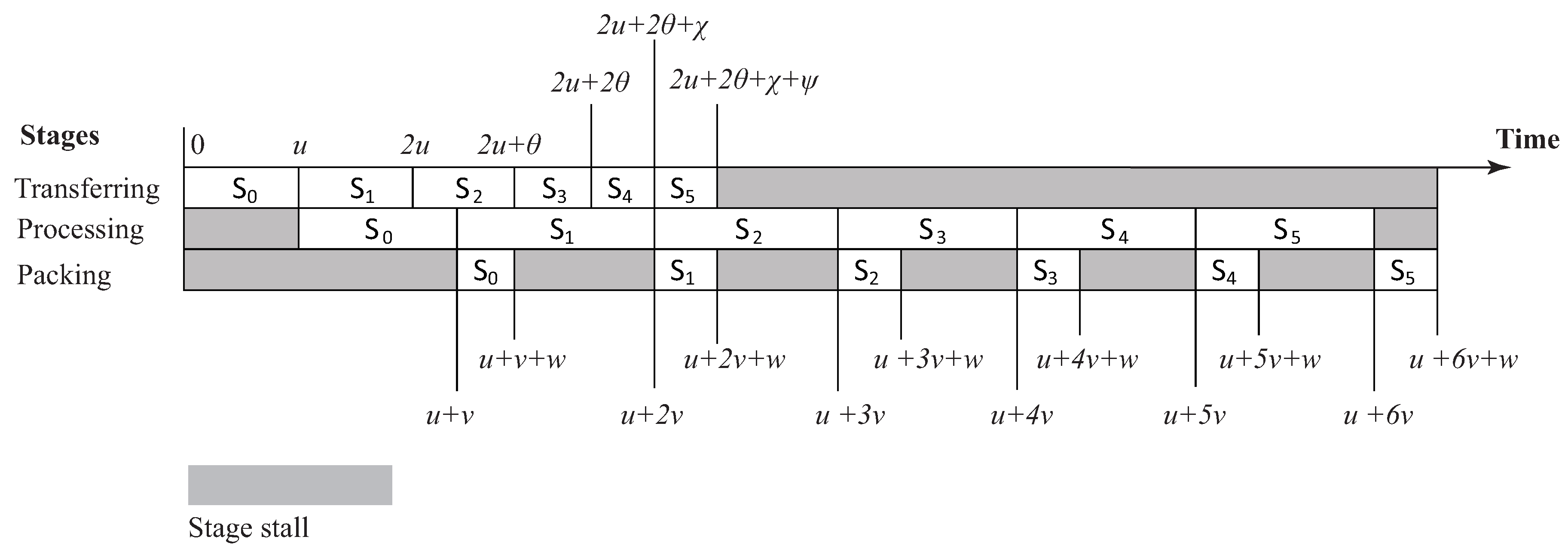
In this first case, we assume that the maximum cost of transfer, u, is larger than the processing cost v. The packing cost is always considered the minimum among the three costs. As indicated by the S M , which was presented is Section 5.1, the transferring costs are not the same for the communicating steps. Here, we describe a general case in which some of the communication steps are more expensive than their processing, while others are not; that is, their processing stage is more expensive. We will use Figure 2 to describe this case. The time is shown in the horizontal axis; some time values have been placed in the bottom of the figure due to space limitations. The horizontal axis shows the three pipeline stages. The grey areas indicate pipeline stage stalls; that is, a stage has no work to do and waits until it becomes busy again. For example, the processing stage cannot be active between times 0 and u, as no data streams have arrived to the proper processing nodes.
Notice that there are two communicating steps, S 0 , S 1 , with a maximum cost of u, which is always the case. Since u > v , one can easily see that the streams corresponding to these steps would be transferred in 2 u time, while their processing will have finished at time 2 u + v . The next two steps, S 2 , S 3 , require a time of θ , where θ < u , but  θ > v . Thus, their cost is still larger compared to the cost of the processing stage. This means that their transfer would be completed at times 2 u + θ and 2 u + 2 θ , respectively, while their processing will have finished at times 2 u + θ + v and 2 u + 2 θ + v , respectively. So far, it can be observed that the processing times are somehow “absorbed” by the transferring times. However, this is not the case for the communication steps, S 4 , S 5 , which require χ and ψ time, where  v > χ > ψ . Therefore, one can notice that the transfer stage for S 4 and the processing stage for S 3 start at time 2 u + 2 θ , but the streams of S 4 would be transferred by 2 u + 2 θ + χ , while the processing of S 3 , which started simultaneously, ends later, at time 2 u + 2 θ + v . Finally, the streams of S 5 will be transferred by 2 u + 2 θ + χ + ψ , and during that time, the processing of S 4 streams takes place. The overall processing terminates at time 2 u + 2 θ + χ + ψ + v . As can be observed, the packing times are totally “absorbed” (overlapped with the times required by the other stages), with the packing of S 5 being the only exception. This adds another w time to the total cost, T C , which gives us
T C = 2 u + 2 θ + χ + ψ + v + w 2 u + [ ( N 2 ) θ ] + v + w
where N is the number of communication steps. We can see that the maximum T C with pipelining is achieved if there are two communication steps of the maximum cost (this is always the case) and all the remaining N 2 steps have a cost of θ (the second largest cost).
Without pipelining, the total cost T C W would be
T C W = 2 ( u + v + w ) + 2 ( θ + v + w ) + ( χ + v + w ) + ( ψ + v + w ) > T C
even for the worst-case scenario for T C .
In the worst-case scenario just described, the TCW is bounded by 2 ( u + v + w ) + [ ( N 2 ) ( θ + v + w ) ] .
Before proceeding to the next case, let us discuss a straightforward case, in which all the communication steps are more expensive compared to processing. This means that u > θ > χ > ψ > v . In such a scenario, the total cost, T C , depends entirely on the first stage (there is a complete overlap with the times required for processing and packing). This makes the total cost somehow smaller compared to the one computed in Equation (14):
T C = 2 u + 2 θ + χ + ψ 2 u + ( N 2 ) θ
and, of course, this is again an improvement compared to the T C W . Further improvement could be achieved if we could find a mechanism that can further reduce the transferring stage times; that is, reducing the communication times of the steps defined by the S M . This will be discussed in Section 7.
(B) The processing stage is always more expensive compared to the transferring stage; v > u > w
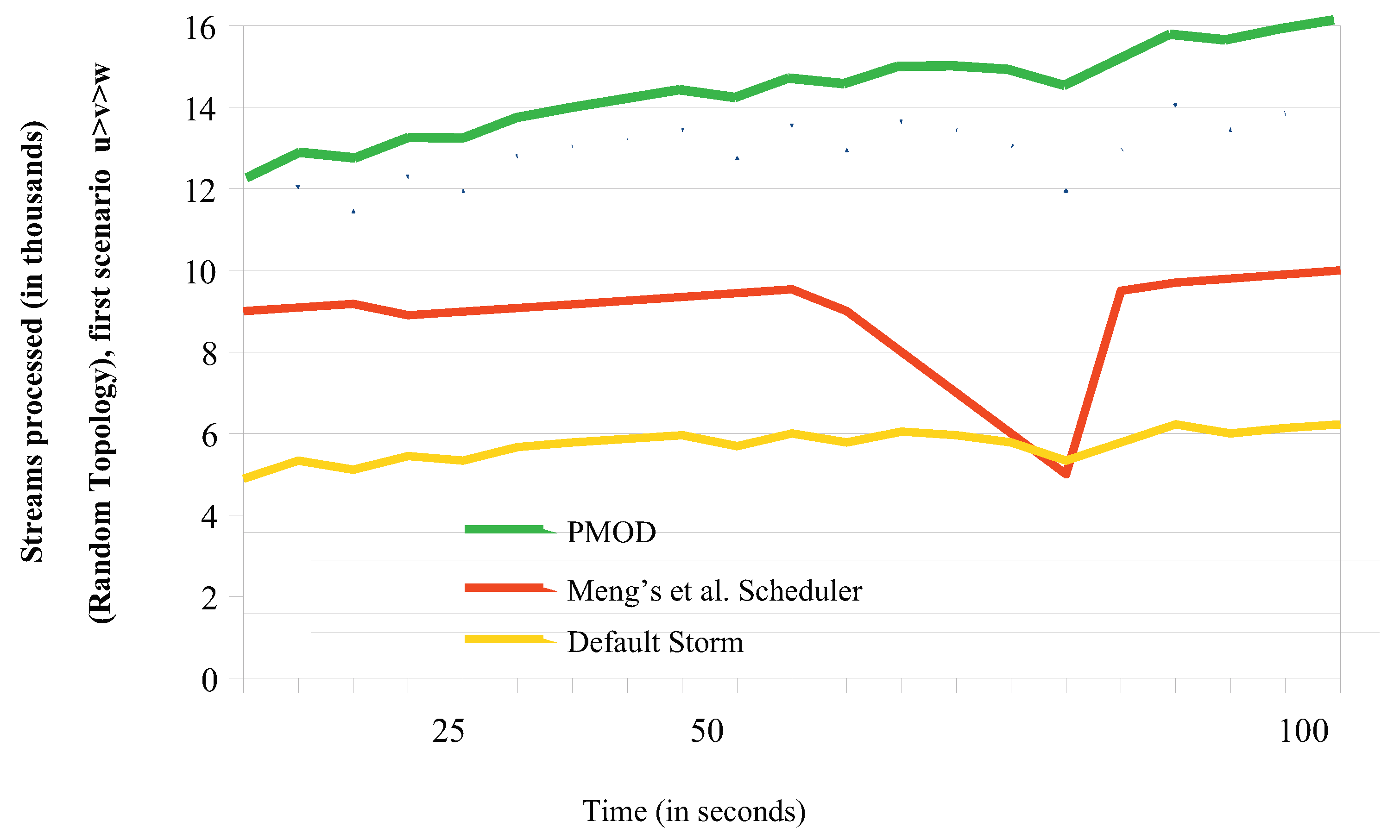
In this scenario (see Figure 3), we assume that the data streams require such an exhausting processing procedure that the processing time overcomes the transferring time; that is, v > u > w . From Figure 3, it is obvious that all of the transferring time and almost all of the packing time overlaps with the processing time. Clearly, the total cost, T C , is
T C = u + 6 v + w or   generally T C = u + N v + w ,
where N is the number of communicating steps.
In this case, further improvements can be made only on an application basis, as the total cost is determined by stream processing. For example, if pipelining can be used to process an application’s data, we can achieve improvements at the processing stage, thus improving the total cost. However, the implementation of a scheduling scheme that is optimal for all the applications is an NP-hard problem.

5.3. Putting the Ideas Together

In this paragraph, we combine all of the ideas discussed in this section to present the method of implementing the PMOD scheduler (see Algorithm 1). Initially, the system parameters N , t are set and read (line 2), and the two distributions, the initial R and the next R , are defined (line 3). Then, the communication classes are computed based on the parameters of R , R . To  define the communication steps, the scheduler implements the two communication steps described in detail in Section 5.1 so that the class table is transformed into a scheduling matrix (lines 5–10). Then, the application DAG (line 12) is read and the proper communications between the spouts/bolts are defined (application specific).
To pipeline the overall processing, the system’s hardware is set to execute three different procedures simultaneously (line 13): implementing the communications defined in one step, processing the data associated to a communicating step and packing the newly processed data for future transfer/processing. The system starts from step k = 0 , as defined by the scheduler. The communications between the node pairs defined in this step are implemented. Now, if  k = 0 , stage S2 has no work to do (line 21); the same holds for stage S3 (line 22). Then, k is incremented by one (line 23), so the three stages are set to work again. Stage 1 implements communication step 1, and stage S2 ( k = 1 > 0 ) implements the processing of the data associated with the previous stage S1 (step 0). The last stage, S2, remains idle, since k < 2 . Once k is incremented again, stage S1 will work on the transmission of data associated with communication step 2, while stage S2 will process the data associated with communication step 1 and stage S2 will pack the data associated with communication step 0. This procedure continues until all the communications have been implemented. If more streams are left unprocessed, k is set back to 0 (the program moves back to line 15) and the repeat block is executed once again.
The complexity of the PMOD scheduler is clearly linear, as it depends on the number of transformations required to change the CT into a single index matrix (SIM) and then the SIM into the scheduling matrix, S M . As the number of these transformations is determined by the number of nodes in the system, PMOD’s complexity is O ( N ) .
Algorithm 1: MOD Scheduler
input: An application graph organized in spouts/bolts of t tasks
    A cluster of N nodes
    Changes in t or N or both, during runtime
output: A dynamic pipelined scheduler, P M O D , with reduced overall cost
1 begin
2   Read parameter changes, that is, new values of t and N
3   Define the distributions R ( i , n , L , x ) and R ( j , q , M , y )
4   Solve Equation (9) to Find all the classes k and produce the Class Table (CT)
5   //Step 1: Transform CT into a Single Index Matrix (SIM)
6   For each node pair ( n , q ) in row k,
7     place the q value to columnn n
8   end For;
9   // Step 2: Mix Class Elements to Produce the Scheduling Matrix ( S M )
10   Interchange α elements of homogeneous classes, that reside in corresponding columns.
11   The rows of the S M correspond to communicating steps between the system’s nodes
12
13   Read the application DAG and define all the communications between components.
14   Define the three pipeline stages (transferring, processing, and packing)
15     k = 0
16   // Organize the three operations in a pipeline fashion:
17    Repeat
18   // Stages S1-S2 are simultaneous and correspond to transferring, processing, packing:
19      S1. Let the transferring stage hardware implement communication step k
20      S2. If  k > 0 , let the processing stage hardware process the data from step k 1
21      S3. If  k > 1 , let the packing stage hardware pack data from step k 2
22      Increment k by one and repeat the simultaneous stages S1-S3.
23     Until all the communications from k communication steps are implemented.
24     If more streams are left unprocessed, go to line 15 and re-execute the pipeline stages.
25 end;

6. Simulation Results and Discussion

For our simulation environment we used a small cluster of five nodes, with an Intel Core i7-8559U Processor system and a clock speed of 2.7 GHz. Furthermore, there was all-to-all communication between the nodes. To conduct our experiments, we used two different topologies: a random topology similar to the one shown in Figure 1 and a linear topology. For both topologies, we assigned four tasks to each bolt/spout, and this number was then changed to five. We ran two sets of simulations for both topologies to examine the two scenarios described in the previous section: (a) some communications steps are more expensive compared to the stream processing, and (b) the processing stage is always more expensive compared to the transferring stage,
For comparison reasons, we chose the default Storm scheduler and Meng’s scheme [21]. The reasoning behind choosing these techniques is that the Storm scheduler is the point of reference for a large percentage of strategies developed in the literature, while Meng’s strategy is also based on the idea of using a matrix model for task scheduling (which offers the advantage of low complexity). The two measures we compared are the total throughput and the load balancing, which are perhaps the most important indicators of a big data system’s performance.

6.1. Throughput Comparisons

To compare the throughputs achieved by the three strategies, we ran four simulation sets in total: for the first two, we used a random topology, and for the other two, we used a linear topology. For both topologies, we applied the two scenarios regarding the timing relationship of the transferring and processing stages.   

6.1.1. Throughput Comparisons for the Random Topology

For the first scenario, we measured the stream parts processed by the system’s nodes. Each stream part was considered as a small group of 50 tuples. We assumed that the first (most expensive) transferring steps defined by the scheduling matrix took more time than their processing, while the last steps (less expensive steps) took less time than their processing. For the most expensive steps defined by the S M , no buffer space was required: the data streams that arrived to the nodes found them idle, so the processing stage was activated immediately and processing started. For the less expensive steps, the data streams had to be buffered, waiting for the completion of processing of the data streams which previously arrived. When more buffering was required, the throughput performance decreased as increasing numbers of data streams were kept waiting in the buffers. Generally, our strategy used less buffer memory as a result of the fact that each node received streams from exactly one other node at each step; thus, some care was taken regarding the data streams received by each task. Moreover, our pipelined scheme reduced the overall time (transferring, processing, packing), as explained in Section 5. This increased the throughput of our work. A disadvantage of Meng’s strategy is the task migration which occurred and added extra overheads to its overall performance. The default Storm strategy has no particular mechanisms to organize the data being transferred; therefore, its performance is generally the worst among all the competitors.
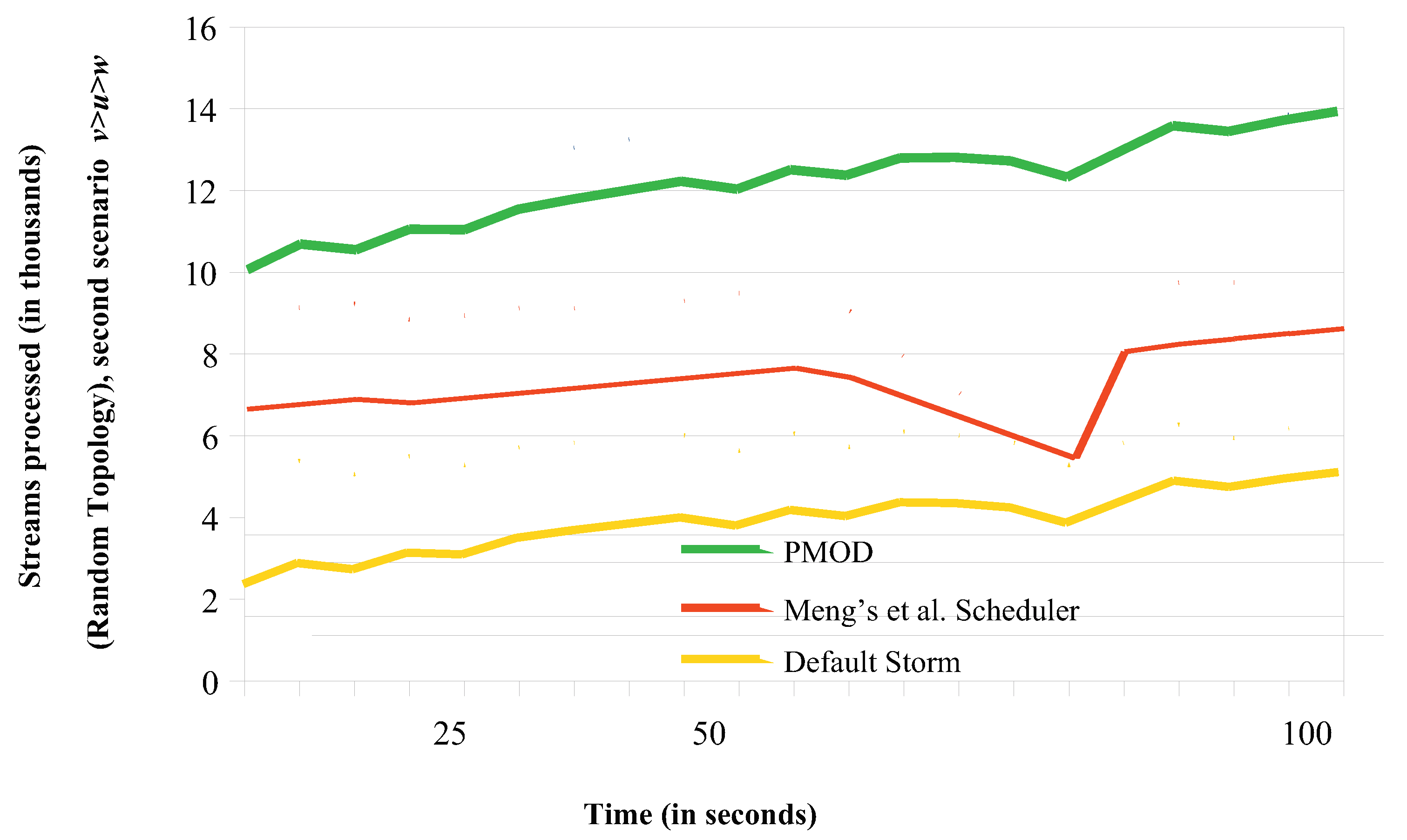
The effect of buffering is clearer in the second scenario. The three strategies appeared to behave in a similar manner, but the number of tuples being processed decreased by an average of about 25%. When v > u , the data streams were transferred quickly, while processing took longer. Again, our strategy outperformed the others due to the data transferring organization in steps and due to pipelining, which reduced the overall processing times.
Finally, we have to emphasize the effects caused by the nature of each application’s topology. When the topology is random, such as the one in Figure 1, then there are cases in which one task may receive data streams from several tasks at the same time. This is also true for our scheme: during a communication step, two tasks that belong to the same source node may transfer the data streams to the same task that belongs to the target source. In the example shown in Figure 1, this can happen during the communication between bolts 2 and 3 and bolt 4. If tasks E,J belong to the same source node and task M belongs to the target node, then two data streams would be transmitted to M during the internode communication. Necessarily, one of the streams has to be buffered. As will be seen in the next set of simulations, all the schemes performed better for the linear topology.
Figure 4 and Figure 5 show the throughput performance for the random topology under the first and second scenarios, respectively.

6.1.2. Throughput Comparisons for the Linear Topology

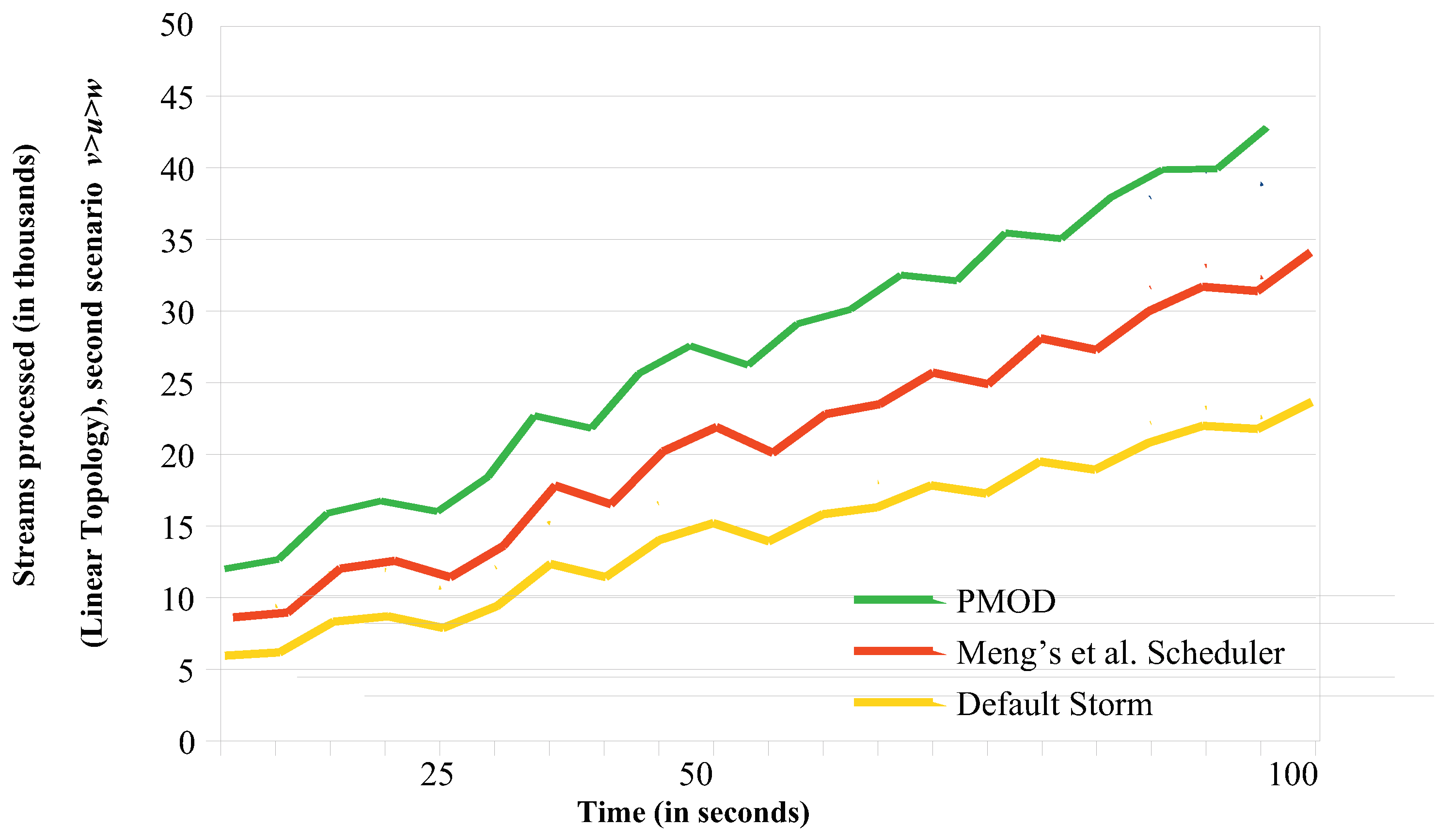
As explained in the first set of experiments, when the application’s topology is linear, less buffering is required, and this has a positive effect on the throughput performance. One can easily see an increase in the numbers of streams being processed, while the curves appear to have an increasing (positive) slope over time, which is not the case for the random topology. Between the two scenarios, again, the first one seems to achieve better performance by an average of 20%, as the second scenario necessarily requires more data streams to be buffered; thus, it adds overheads. Again, in both cases, our strategy outperforms its competitors. Figure 6 and Figure 7 show the throughput performance for the random topology under the first and second scenarios, respectively.

6.2. Load Balancing Comparisons

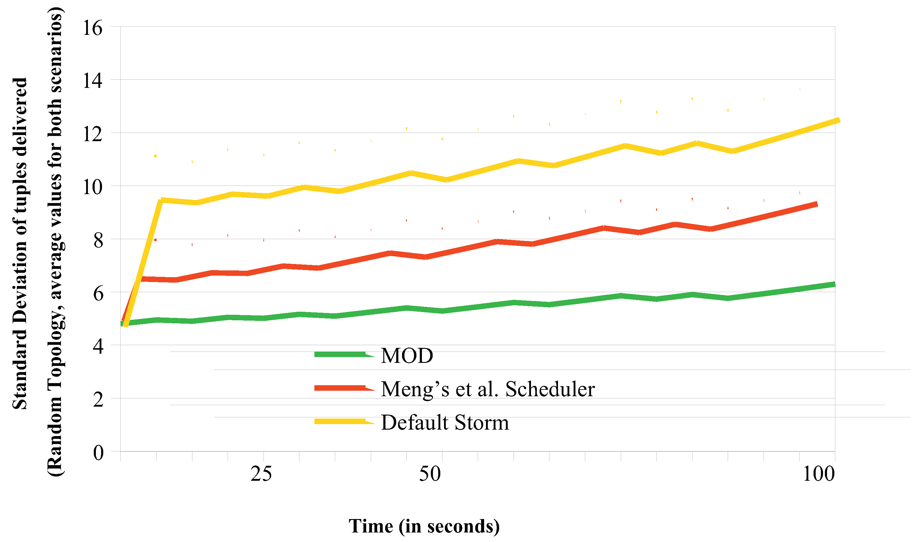
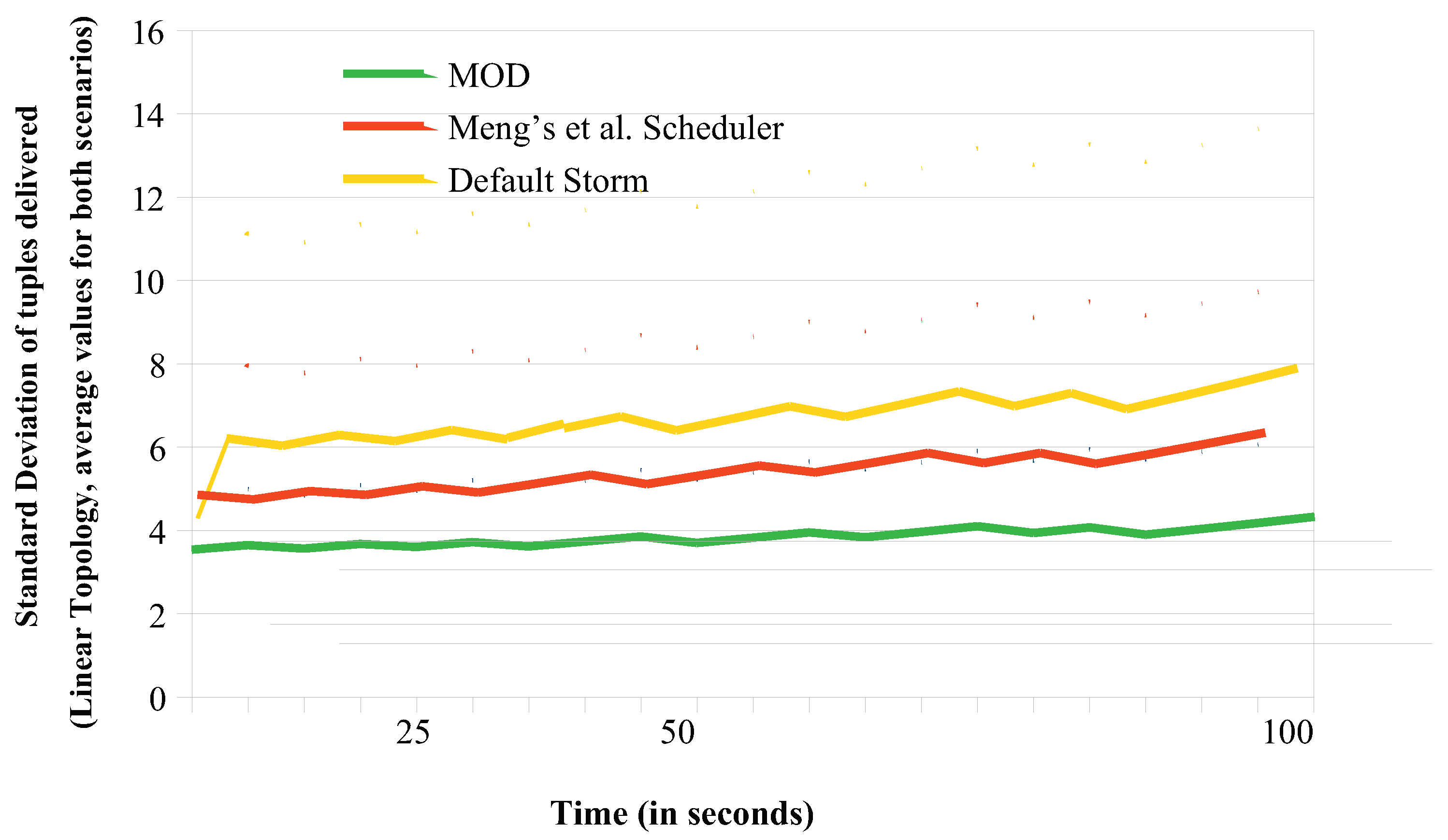
To examine load balancing, we compared the average standard deviation of the load being delivered to each node (see Figure 8 and Figure 9). In Figure 8, we show the results of the experiments conducted on the random topology, and in Figure 9, we show the results found by experimenting on the linear topology (the settings are similar to those in the previous experiments). The results shown are the average standard deviation values, as obtained by the application of the two scenarios on each topology. The standard deviation is computed at regular intervals of 5 s. Apparently, as the standard deviation increases, less load balancing is achieved.
Generally two things need to mentioned: first, our strategy offers almost ideal balancing for both topologies as it is based on the fact that, at each step, there is a one-to-one communication among the system nodes. Thus, the standard deviation values for our strategy are reduced compared to those computed for the competitors’ strategies. Our scheme is not affected by the growing number of tuples added to the nodes, as this is done in a balanced way. The other strategies seem to be more affected by the increasing number of tasks being delivered. In particular, the default scheduler seems to become quite “unbalanced”, while Meng’s et al. strategy is affected by the changes in the task positions, which are applied during runtime. As a result, some tasks become increasingly overloaded. Apparently, all the strategies appear to be more balanced when the topology is linear (note that the standard deviation values are smaller in this case). The reason for this was explained above when we presented the throughput experiments; for a random application topology, the general case (even in our strategy) is that the tasks may not receive equal sized data streams.

7. Conclusions—Future Work

This work presented a pipelined dynamic task scheduling approach with linear complexity, which was designed to handle system changes (in terms of the number of nodes or tasks) for applications that require heavy communication between nodes and tasks. Our approach is organized in a set of communication steps, where there is a one-to-one communication between the system’s nodes. The basic procedures (transferring, processing and packing) required by a big data processing system are pipelined using three different stages.
As a result of our organization in steps, the buffering space required is reduced, resulting in higher throughput, as a percentage of streams are processed immediately as they arrive to the target node. A second advantage of our strategy is the almost perfect load balancing, as a result of the way that communication is organized. The experimental results obtained have shown that our scheme (as well as the competitive schemes we used for comparisons) generally performs better for linear topologies and when the transfer times are generally larger compared to the processing times (first scenario). When processing requires more time, we observed a reduction of performance.
In the future, we plan to extend this work in order to produce faster processing and communication time. One concept under investigation is the use of more transformations for the schedule matrix ( S M ) in order to break down the most expensive communications into fewer separated steps. Then, the less expensive steps would also be gathered into separate steps; this may result in reduced communication times. Furthermore, we plan to study certain applications and try to improve their performance using some of the ideas presented in this work; for example, pipelining the operations required by a certain application could reduce the overall processing time.

Author Contributions

Conceptualization, S.S., methodology, S.S.; software, S.S. and S.A.; validation, S.S. and S.A.; formal analysis, S.S., and S.S.; investigation, S.A., resources, S.A., writing—original draft preparation, S.S.; writing—review and editing, S.S., S.A.; funding acquisition, S.A. All authors have read and agreed to the published version of the manuscript.

Funding

This research was funded by the University of Western Macedonia, Faculty of Education, Department of Early Childhood Education.

Conflicts of Interest

The authors declare no conflict of interest.

References

  1. Tantalaki, N.; Souravlas, S.; Roumeliotis, M. A review on Big Data real-time stream processing and its scheduling techniques. Int. J. Parallel Emerg. Distrib. Syst. 2019. [Google Scholar] [CrossRef]
  2. Tantalaki, N.; Souravlas, S.; Roumeliotis, M.; Katsavounis, S. Linear scheduling of big data streams on multiprocessor sets in the cloud. In Ser. WI’19, Proceedings of the IEEE/WIC/ACM International Conference on Web Intelligence, Thessaloniki, Greece, 14–17 October 2019; ACM: New York, NY, USA, 2019; pp. 107–115. [Google Scholar]
  3. Apache Software Foundation. Apache Storm. Available online: http://storm.apache.org/ (accessed on 5 June 2019).
  4. Apache Software Foundation. Spark Streaming-Apache Spark. Available online: http://spark.apache.org/streaming/ (accessed on 5 June 2019).
  5. Apache Software Foundation. Apache Samza—A Distributed Stream Processing Framework. Available online: https://samza.apache.org (accessed on 5 June 2019).
  6. Apache Software Foundation. Apache Flink-Stateful Computations over Data Streams. Available online: https://flink.apache.org/ (accessed on 5 June 2019).
  7. Souravlas, S. ProMo: A Probabilistic Model for Dynamic Load-Balanced Scheduling of Data Flows in Cloud Systems. Electronics 2019, 8, 990. [Google Scholar] [CrossRef] [Green Version]
  8. Aniello, L.; Baldoni, R.; Querzoni, L. Adaptive Online Scheduling in Storm. In Proceedings of the 7th ACM International Conference on Distributed Event-based Systems (DEBS ’13), Arlington, TX, USA, 29 June–3 July 2013; pp. 207–218. [Google Scholar] [CrossRef]
  9. Eskandari, L.; Huang, Z.; Eyers, D. P-Scheduler: AdaptiveHierarchical Scheduling in Apache Storm. In Proceedings of the Australasian Computer Science Week Multiconference (ACSW ’16), Canberra, Australia, 2–5 February 2016; Article 26. p. 10. [Google Scholar] [CrossRef]
  10. Eskandari, L.; Mair, J.; Huang, Z.; Eyers, D. Iterative scheduling for distributed stream processing systems. In Ser.DEBS ’18, Proceedings of the 12th ACM International Conference on Distributed and Event-Based Systems, Hamilton, New Zealand, 25–29 June 2018; ACM: New York, NY, USA, 2018; pp. 234–237. [Google Scholar]
  11. Shukla, A.; Simmhan, Y. Model-driven scheduling for dis-tributed stream processing systems. J. Parallel Distrib. Comput. 2018, 117, 98–114. [Google Scholar] [CrossRef] [Green Version]
  12. Eidenbenz, R.; Locher, T. Task allocation for distributed stream pro-cessing. In Proceedings of the IEEE INFOCOM 2016—The 35th Annual IEEE InternationalConference on Computer Communications, San Francisco, CA, USA, 10–14 April 2016; pp. 1–9. [Google Scholar]
  13. Xiang, D.; Wu, Y.; Shang, P.; Jiang, J.; Wu, J.; Yu, K. Rb-storm: Resourcebalance scheduling in Apache storm. In Proceedings of the 2017 6th IIAI International Congress on Advanced Applied Informatics (IIAI-AAI), Hamamatsu, Japan, 9–13 July 2017; pp. 419–423. [Google Scholar]
  14. Al-Sinayyid, A.; Zhu, M. Job scheduler for streaming applications inheterogeneous distributed processing systems. J. Supercomput. 2020. [Google Scholar] [CrossRef]
  15. Janssen, G.; Verbitskiy, I.; Renner, T.; Thamsen, L. Scheduling streamprocessing tasks on geo-distributed heterogeneous resources. In Proceedings of the 2018 IEEE International Conference on Big Data (Big Data), Seattle, WA, USA, 10–13 December 2018; pp. 5159–5164. [Google Scholar]
  16. Peng, B.; Hosseini, M.; Hong, Z.; Farivar, R.; Campbell, R. R-storm: Resource-aware scheduling in storm. In Proceedings of the 16th Annual Middleware Conference, Ser. Middleware ’15, Vancouver, BC, Canada, 7–11 December 2015; pp. 149–161. [Google Scholar]
  17. Smirnov, P.; Melnik, M.; Nasonov, D. Performance-aware schedulingof streaming applications using genetic algorithm. Procedia Comput. Sci. 2017, 108, 2240–2249. [Google Scholar] [CrossRef]
  18. Fu, T.Z.J.; Ding, J.; Ma, R.T.B.; Winslett, M.; Yang, Y.; Zhang, Z. DRS: Dynamic Resource Scheduling for Real-Time Analyticsover Fast Streams. In Proceedings of the IEEE 35th International Conference on Distributed Computing Systems, Columbus, OH, USA, 29 June–2 July 2015; pp. 411–420. [Google Scholar] [CrossRef] [Green Version]
  19. Cardellini, V.; Grassi, V.; Presti, F.L.; Nardelli, M. Optimal Operator Replication and Placement for Distributed Stream Processing Systems. ACM Sigmetrics Perform. Eval. 2017, 44, 11–22. [Google Scholar] [CrossRef]
  20. Xu, J.; Chen, Z.; Tang, J.; Su, S. T-Storm: Traffic-AwareOnline Scheduling in Storm. In Proceedings of the 2014 IEEE 34th International Conference on Distributed Computing Systems (ICDCS ’14), Madrid, Spain, 30 June–3 July 2014; pp. 535–544. [Google Scholar] [CrossRef]
  21. Chen, M.-M.; Zhuang, C.; Li, Z.; Xu, K.-F. A Task Scheduling Approach for Real-Time Stream Processing. In Proceedings of the International Conference on Cloud Computing and Big Data, Wuhan, China, 12–14 November 2014; pp. 160–167. [Google Scholar] [CrossRef]
  22. Liu, Y.; Wang, K.; Yu, Y.; Qi, J.; Sun, Y. A dynamic assignment scheduling algorithm for big data stream processing in mobile Internet services. Pers. Ubiquitous Comput. 2016, 20, 373–383. [Google Scholar] [CrossRef]
  23. Floratou, A.; Agrawal, A.; Graham, B.; Rao, S.; Ra-masamy, K. Dhalion: Self-regulating Stream Processing. Proc. VLDB Endow. 2017, 10, 1825–1836. [Google Scholar] [CrossRef]
  24. Souravlas, S.; Roumeliotis, M. A pipeline technique for dynamic data transfer on a multiprocessor grid. Int. J. Parallel Program. 2004, 32, 361–388. [Google Scholar] [CrossRef]
  25. Souravlas, S.; Roumeliotis, M. On further reducing the cost of parallel pipelined message broadcasts. Int. J. Comput. Math. 2006, 83, 273–286. [Google Scholar] [CrossRef]
  26. Souravlas, S.; Roumeliotis, M. Scheduling array redistribution with virtual channel support. J. Supercomput. 2015, 71, 4215–4234. [Google Scholar] [CrossRef]
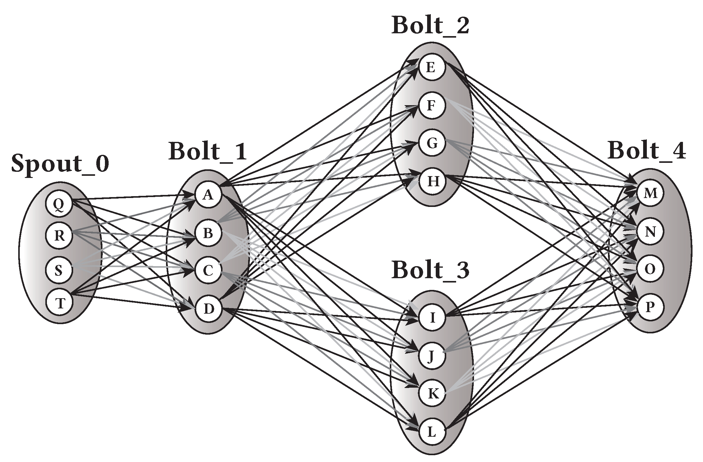
Figure 1. Task interconnection for a random application.
Applsci 10 04796 g001
Figure 2. Pipelined scheduling, u > v > w .
Applsci 10 04796 g002
Figure 3. Pipelined scheduling, v > u > w .
Applsci 10 04796 g003
Figure 4. Throughput comparisons with a random topology for the first scenario: ( u > v > w ) .
Applsci 10 04796 g004
Figure 5. Throughput comparisons with a random topology for the second scenario: ( v > u > w ) .
Applsci 10 04796 g005
Figure 6. Throughput comparisons with a linear topology for the first scenario: ( u > v > w ) .
Applsci 10 04796 g006
Figure 7. Throughput comparisons with a linear topology for the second scenario: ( v > u > w ) .
Applsci 10 04796 g007
Figure 8. Load balancing comparisons with a random topology for both scenarios.
Applsci 10 04796 g008
Figure 9. Load balancing comparisons with a random topology for both scenarios.
Applsci 10 04796 g009
Table 1. Class table (CT) for N = Q = 6 , t = 4 , s = 5 .
ClassCommunicating Nodesc
0(0,0), (3,0), (1,2), (4,2), (2,4), (5,4)4
1(0,1), (3,1), (1,3), (4,3), (2,5), (5,5)4
2(2,0), (5,0), (0,2), (3,2), (1,4), (4,4)3
3(2,1), (5,1), (0,3), (3,3), (1,5), (4,5)3
4(1,0), (4,0), (2,2), (5,2), (0,4), (3,4)3
5(1,1), (4,1), (2,3), (5,3), (0,5), (3,5)3
Table 2. Communication latencies among Q 2 node communications.
Latency q Number of Communicating Nodes Exhibiting This Latency
0 = 0 Q
1 = 1 2 ( Q 1 )
2 = 2 2 ( Q 2 )
3 = 3 2 ( Q 3 )
4 = 4 2 ( Q 4 )
q 1 = Q 1 2