Multiclass Non-Randomized Spectral–Spatial Active Learning for Hyperspectral Image Classification

Abstract

Active Learning (AL) for Hyperspectral Image Classification (HSIC) has been extensively studied. However, the traditional AL methods do not consider randomness among the existing and new samples. Secondly, very limited AL research has been carried out on joint spectral–spatial information. Thirdly, a minor but still worth mentioning factor is the stopping criteria. Therefore, this study caters to all these issues using a spatial prior Fuzziness concept coupled with Multinomial Logistic Regression via a Splitting and Augmented Lagrangian (MLR-LORSAL) classifier with dual stopping criteria. This work further compares several sample selection methods with the diverse nature of classifiers i.e., probabilistic and non-probabilistic. The sample selection methods include Breaking Ties (BT), Mutual Information (MI) and Modified Breaking Ties (MBT). The comparative classifiers include Support Vector Machine (SVM), Extreme Learning Machine (ELM), K-Nearest Neighbour (KNN) and Ensemble Learning (EL). The experimental results on three benchmark hyperspectral datasets reveal that the proposed pipeline significantly increases the classification accuracy and generalization performance. To further validate the performance, several statistical tests are also considered such as Precision, Recall and F1-Score.

1. Introduction

Hyperspectral imaging (HSI) examines the reflection of light of an object across a wide range of electromagnetic spectra instead of just associating primary colors to a pixel [1]. Light interacting with a pixel is divided into several bands in order to render complete information about a target [2]. Therefore, HSI has gained significant importance in many applications including. but not limited to, chemical imaging [3], agriculture [4], surveillance [5], remote sensing [6], household materials [7], and environmental sciences [8]. The main challenge of HSI analysis is its high dimensional characteristic of data due to a large number of bands with significantly high resolution across the electromagnetic spectrum. Therefore, the classification of HSI data is a complex and challenging task [9].

Some widely used supervised classification approaches for HSI analysis are Multinomial Logistic Regression (MLR) [10], Support Vector Machine (SVM) [11], Maximum Likelihood [10,12], Ensemble Learning (EL) [13,14], Random Forests (RF) [15,16], Deep Learning (DL) [17,18,19], Transfer Learning [20,21], k-Nearest Neighbors (KNN) [22] and Extreme Learning Machine (ELM) [23]. The major limitation of supervised HSI classification is the poor performance due to the Hughes phenomena [24]. It occurs when the ratio of spectral bands is significantly less as compared to the labeled training samples available in hyperspectral data [25]. The acquisition of most informative labeled training examples is often an expensive and time-intensive task as it generally requires human experts or a ground campaign [26].

Limited availability of reliable labeled training examples brings the idea to utilize semi-supervised learning [27]. The basic concept of such a learning mechanism is that new training examples can be obtained from the unlabeled data, without considerable time and cost, by utilizing limited available labeled examples [28,29]. A few examples of such techniques are kernel techniques [30], such as EL techniques [31,32], Tri-training [33,34] and Graph-based learning [35]. However, the performance of these techniques is relatively low when combined with the limited availability of reliable labeled training examples for high dimensional datasets e.g., hyperspectral datasets.

To cope with the aforesaid issues, one of the commonly used semi-supervised approaches is the expansion of the initial training set by efficiently utilizing unlabeled data. This method is known as Active Learning (AL) which significantly improves the performance of classification techniques by adding new examples in the training set for the next cycle of training, unless a stopping criteria is met, i.e., required classification accuracy. Depending on the criteria of adding new examples to the training set, AL techniques can be categorized as stream or pool-based and the selection of new examples is based on ranking scores that are reckoned from measures like representativeness, uncertainty, variance, inconsistency and error [6].

For instance, uncertainty measures consider the unlabeled examples more important than those close to the class boundary of the current classification results. Representativeness selects those unlabeled examples as more significant, which can represent a new group of examples, i.e., a cluster. Inconsistency assumes the unlabeled samples more useful and has high predictive divergence among multiple classifiers [36]. However, all these methods have one major limitation which is randomness among the samples. The new training samples are always selected with certain criteria without considering whether the selected samples are similar to the previously selected samples or not which induces the redundancy among the samples. The other main issue with many AL methods is their stopping criteria which are most certainly based on the accuracy number.

This paper proposed a multi-class non-randomized AL method based on Multinomial Logistic Regression (MLR)-LORSAL classifier [31,37] in conjunction with fuzziness [6] as sample selection method whilst exploiting both spatial and spectral information of hyperspectral data. We further compared the MLR-LORSAL against various well-known classifiers such as; SVM, ELM, KNN and EL. Each classifier is further evaluated against three benchmark sample selection methods in addition to fuzziness. These sample selection methods include Breaking Ties (BT) [38], Mutual Information (MI) [39] and Modified Breaking Ties (MBT) [39]. The motivation of our current work is to investigate several state-of-the-art sample selection and classification techniques with predefined dual stopping criteria and to properly generalize them for remotely sensed hyperspectral datasets.

The paper is structured as follows. Section 2 discuss the pipeline proposed in this work. Section 3 presents the experimental process and performance measurement metrics. Section 4 contains the information regarding the experimental results and datasets. Finally Section 5 concludes the paper with possible future directions.

2. Methodology

This work addressed the issue of a small training set while classifying the high-dimensional multi-class HSI data by introducing a fuzziness MLR-based classifier which actively selects the data based on two main aspects: first, is the sample’s fuzziness and second is the non-randomized selection of samples to avoid redundancy among them. Furthermore, we compared it with four benchmark AL techniques in association with four different classifiers. We evaluated AL techniques on a pool of diverse samples in each iteration thus minimizing the redundancy among selected samples.

2.1. Hyperspectral Data Formulation

The symbols used in this work has been illustrated in

Table 1. Explanation of used Symbols.

Symbols	Explanations
X	Hyperspectral Data Cube, where $X={[x_1,x_2,x_3,\dots ,x_L]}^T\in R^{L\times (M\times N)}$
L	Number of Bands in Hyperspectral Image Cube.
$M\times N$	Number of Samples in each Band of Hyperspectral cube.
C	Total Number of Classes in Hyperspectral Cube.
n	Total Number of Initial Training Samples.
m	Total Number of Initial Test Samples.
h	Total Number of Queried Sample
$\widehat{m}$	Number of Samples Selected in each Iteration where $\widehat{m}\ll m$ also $n+\widehat{m}\ll m$
$\mathcal{X}$	Index of Selected Samples.
$x_i$	ith Spectral Sample and $i=1,2,3,\cdots ,n$.
$y_j$	Class label of ith Spectral Sample, where $j=1,2,3,\cdots ,C$
$X_T$	Training Set consist of n Samples.
$X_V$	Initial Test Set consist of m Samples, where $n<<m$ and $(X_T\cap X_V)=\varnothing$
$\mu$	Membership Matrix, i.e., output of classifier
$u_{ij}$	Membership of ith sample for jth class
$F\left({\mu }_{ij}\right)$	Fuzziness computed through $u_{ij}$
${\alpha }_j$	Selected Reference Training Samples
${\beta }_{ij}$	Spectral Angular Distance among the New and Existing Training Samples
$OA$	Overall Accuracy
$\kappa$	Kappa metric
TP	True Positive
FP	False Positive
TN	True Negative
FN	False Negative
MI	Mutual Information
BT	Breaking Ties
MBT	Modified Breaking Ties

. Let us assume a Hyperspectral dataset can be expressed as $X={[x_1,x_2,x_3,\dots ,x_L]}^T\in R^{L\times (M\times N)}$ consisting of $M\times N$ samples associated with C classes per band with total L bands, in which each sample is represented as $(x_i,y_j)$, where $y_j$ is the class label of $x_i$ sample. In a nutshell ith sample belongs to jth class.

Furthermore, suppose that $n=50$ number of initial labeled training samples (given equal representation to each class) are chosen from X to form the training set $X_T=\left\{(x_i,y_j)\right\}$ where $i=1,2,3,\cdots ,n$ and $j=1,2,3,\cdots ,C$. The remaining samples make the validation set $X_V={\left\{(x_i,y_i)\right\}}_{i=1}^m$. It should be noted that $n<<m$, and $(X_T\cap X_V)=\varnothing$.

2.2. Multinomial Logistic Regression via Splitting and Augmented Lagrangian (MLR-LORSAL)

An NP classifier modeled using $X_T$ is tested on $X_V$, outputs a matrix $\mu$ of $m\times C$ dimensions whose entries correspond to NP outputs (i.e., least-square estimation) of a classifier. Let $u_{ij}$ represent the membership of ith sample for jth class. Various methods are proposed for the transformation of least square estimation into the posteriori probabilities [36,38]. These methods are expensive in terms of computations due to two main aspects: first, in order to estimate $y_i$, they need to approximate the posterior distribution in the case of a Bayesian framework. Secondly, they restrict the training output between 0 and 1. Such methods compute the approximated posterior probabilities in the form of least squares regression i.e., $f(x_i,{\mu }_j)=p({\mu }_j,x_i)$ [40]. An alternate to the least squares approach which outputs the probabilities in $[0-1]$ range is MLR which is computed as [40,41]:

$$p{\left(y_i\right)}^k=1|(x_i,w)=\frac{exp\left(w^{k}h\left(x_i\right)\right)}{{\sum }_{k=1}^{K}exp\left(w^{k}h\left(x_i\right)\right)}$$

(1)

where $h\left(x\right)={[h_1\left(x\right),\cdots ,h_L\left(x\right)]}^T$, mostly termed as features, is a vector of L fixed functions of the input, $w={[w^1,\cdots ,w^{L-1}]}^T$. Since the density function represented in Equation (1) is independent of translations of the regressors $w^L$, we take $w^L=0$. Therefore, the posteriori probabilities are computed by using LORSAL algorithm as similar to the work [37]. $h\left(x_i\right)=[1,{\mu }_{(x,x_1)},\cdots ,{\mu }_{(x,x_L)}]$, where ${\mu }_{(x_i,x_j)}=\mu (x_i,x_j)$ are symmetric kernel functions. RBF has been widely used for HSI classification as it improves the data separability in the transformed space [41,42].

$$\mu (x_i,x_j)=\frac{-exp(\parallel x_i-x_j{\parallel }^2)}{2{\sigma }^2}$$

(2)

From RBF output, a membership matrix ${\mu }_{ij}$ is obtained, which must satisfy the properties [6,25] ${\sum }_{j=1}^C{\mu }_{ij}=1$ and $0<{\sum }_{i=1}^N{\mu }_{ij}<1$ where ${\mu }_{ij}\in [0,1]$ and ${\mu }_{ij}={\mu }_j\left(x_i\right)$ represents the membership of sample i for the jth class [25]. If the approximated posterior probability is close to 1, it represents the true class, whereas wrong class if the probability is close to 0. AL techniques do not need exact probabilities, but they require a ranking of approximated probabilities which makes it easier to calculate the fuzziness [6].

The fuzziness $F\left({\mu }_{ij}\right)$ from the membership matrix ${\mu }_{ij}$ can be expressed as in Equation (3) and it should satisfy the properties defined below [6,43].

$$F\left({\mu }_{ij}\right)=\frac{-1}{m\times C}\sum _{i=1}^m\sum _{j=1}^C[{\mu }_{ij}log{\mu }_{ij}+(1-{\mu }_{ij})log(1-{\mu }_{ij}))]$$

(3)

• $F\left({\mu }_{ij}\right)=0$ iff ${\mu }_{ij}$ is a crisp set.
• $F\left({\mu }_{ij}\right)$ is maximum if ${\mu }_i=0.5$.
• If ${\mu }_{ij}<<{\sigma }_{ij}$ then $F\left({\mu }_{ij}\right)>>F\left({\sigma }_{ij}\right)$ where ${\mu }_{ij}<<{\sigma }_{ij}\iff min(0.5,\mu \left(i\right))\ge min(0.5,\sigma \left(i\right))$ and $min(0.5,\mu (i\left)\right)\le max(0.5,\sigma (i\left)\right)$
• $F({\mu }_{ij}\cup {\sigma }_{ij})+F({\mu }_{ij}\cap {\sigma }_{ij})=F\left({\mu }_{ij}\right)+F\left({\sigma }_{ij}\right)$

where ${\mu }_{ij}$ and ${\sigma }_{ij}$ are fuzzy sets. We first associate the $F\left(\mu \right)$ with actual and predicted class labels and validation set $X_V$. Then this set is sorted in a descending manner according to the $F\left(\mu \right)$ values. After that $\widehat{m}$ number of misclassified samples having higher fuzziness (i.e., $F\left(\mu \right)>>0.7$ and $\widehat{m}\ll m$) values are heuristically selected. We randomly select a reference training sample (${\alpha }_j$) from each class to compute the spectral angle using a Spectral Angle Mapper, which takes the $co{s}^{-1}$ based dot product among the test samples to a reference sample as follows:

$${\beta }_{ij}=\sum _{j=1}^C\sum _{i=1}^{\widehat{m}}\left(co{s}^{-1}\frac{{\alpha }_j·x_{ij}}{\sqrt{{\alpha }_j^2}\sqrt{x_{ij}^2}}\right)$$

(4)

$$\mathcal{X}=\underset{i\in \widehat{m}|X_V}{argmax}\left(d\left({\beta }_{ij}\right)\right)$$

(5)

where $\mathcal{X}$ preserve the information from those samples which have maximum distance among the same class. $\mathcal{X}$ denotes the index of the unlabeled sample that will be included in the pool. Please note that here we used a soft threshing scheme to balance the number of classes in both training and selected samples. This process picks the samples in a non-randomized way to avoid redundancy not only among the pool of new samples but also with the samples that are already added to the training set. We follow the strategy of keeping the pool of $\widehat{m}$ new samples balanced, which gives equal representation to all classes via softening the thresholds at run time. The complete pipeline is presented in Algorithm 1.

Algorithm 1: Pipeline of Proposed Algorithm.

3. Experimental Process

The performance of our proposed pipeline is validated on 3 benchmark HSI datasets that are publicly available and acquired by two different sensors, i.e., Reflective Optics System Imaging Spectrometer (ROSIS) and Airborne Visible/Infrared Imaging Spectrometer (AVIRIS) sensor. These 3 datasets are Salinas, Indian Pines and Pavia University (PU). More information on these datasets can be found in [9,44].

Furthermore, we evaluated our proposed pipeline against five diverse classifiers which are Support Vector Machine (SVM), K-Nearest Neighbors (KNN), Ensemble learning (EL) methods i.e., Gradient Boost (GB) & Logistic Boost (LB) and Extreme Learning Machine (ELM) [45]. We choose these classifiers for comparison purposes because they have been broadly studied for HSI classification. The performance of our proposed pipeline and the aforementioned classifiers is evaluated using two benchmark metrics: Overall Accuracy (OA) and kappa $\left(\kappa \right)$ coefficient [25]. Furthermore, to check the statistical significance of our proposed pipeline, several statistical measures are taken into accounts, such as Precision, Recall and F1-score. All these metrics are computed as follows:

$$OA=\frac{1}{C}\sum _{i=1}^{C}T{P}_i$$

(6)

$$Precision=\frac{1}{C}\sum _{i=1}^C\frac{T{P}_i}{T{P}_i+F{P}_i}$$

(7)

$$Recall=\frac{1}{C}\sum _{i=1}^C\frac{T{P}_i}{T{P}_i+F{N}_i}$$

(8)

$$F1-Score=\frac{2\times (Recall\times Precision)}{(Recall+Precision)}$$

(9)

$$\kappa =\frac{P_o-P_e}{1-P_e}$$

(10)

where

$$P_o=\frac{TP+TN}{TP+FN+FP+TN}$$

(11)

$$P_e=P_Y+P_N$$

(12)

$$P_Y=\frac{TP+FN}{TP+FN+FP+TN}\times \frac{TP+FN}{TP+FN+FP+TN}$$

(13)

$$P_N=\frac{FP+TN}{TP+FN+FP+TN}\times \frac{FN+TN}{TP+FN+FP+TN}$$

(14)

where TP, FP, TN and FN are true positive, false positive, true negative and false negative computed from the confusion matrix, respectively. Moreover, to show that our proposed pipeline is commensurable, we evaluated it against four well-known sample selection methods: Mutual Information (MI), Breaking Ties (BT) and Modified Breaking Ties (MBT).

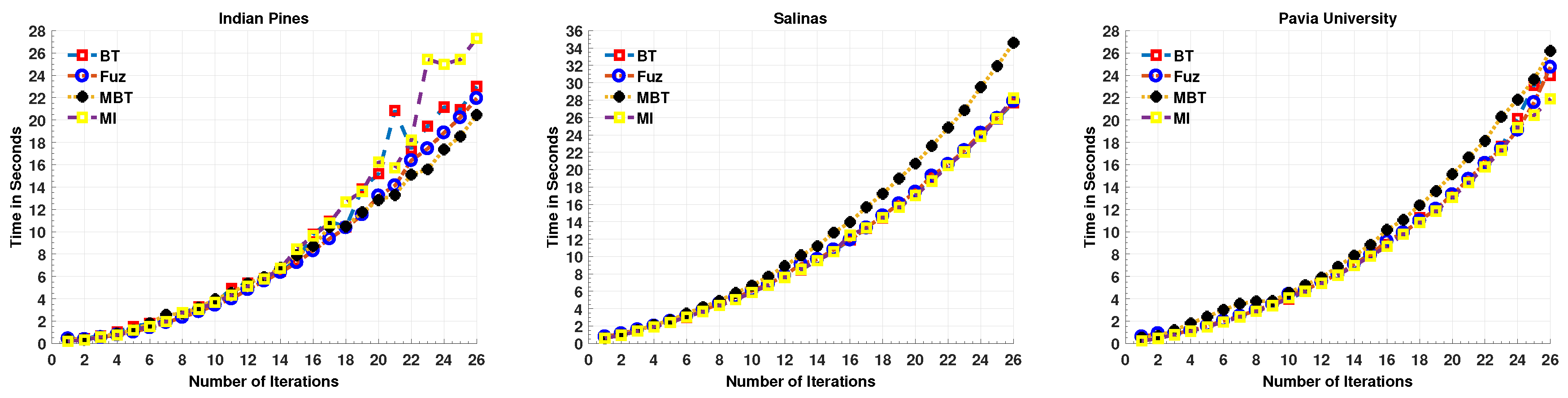
• Mutual Information (MI): Selects the samples by maximizing the mutual information between the classifier and class labels and can obtain samples from the complicated region [39].
• Breaking Ties (BT): Selects the samples by minimizing the distance of the two classes having the highest posterior probabilities, and can choose samples from the boundary regions [46]. In the multiclass scenario, BT can be utilized by finding the difference between the first two most probable classes.
• Modified Breaking Ties (MBT): Adds more diverse samples as compared to MI and BT. The MBT algorithm follows two important steps: first, it selects samples from the unlabeled pool with the same maximum a posteriori (MAP) estimation; and then choose the samples from the most complicated region [46].

In all experiments, 50 samples were selected from the whole HSI data for the initial training dataset and in each iteration of AL process, $h=50$ samples are actively added to the training dataset. The process is repeated until we achieve the desired accuracy of ≥85% for at least one classifier or training set size reaches up to $h=2500$ samples.

SVM is evaluated with polynomial kernel function and in the case of ELM, [1–500] hidden neurons are selected. Similarly, tree-based methods are used to train the ensemble classifiers from a range of [1–100] trees and kNN parameter k is set to [2–20]. All the parameters are adjusted carefully while setting up the experiments. All the experiments are carried out on cluster using MATLAB (2017a) on Intel Core (TM) i7-7700K CPU 2.40 GHz, 1962 MHz, Ubuntu 16.01.5 LTS, CUDA completion tools, release 7.5, V7.5.17 with 65 GB RAM.

4. Experimental Datasets and Results

For the purpose of experimental design, we used five-fold-cross-validation to evaluate the performance of our proposed pipeline. From the results, one can conclude that our proposed approach significantly enhances the classification performance with comparatively less computational time.

This section enlists the experimental results obtained by several sample selection methods with various types of classifiers. These classifiers include Support Vector Machine (SVM), k-Nearest Neighbours (KNN), Ensemble Learning (EL) and Extreme Learning Machine (ELM). The important parameters for all the experimental classifiers mentioned above are carefully tuned and to avoid bias, all the experiments are carried out under the same settings that maximize performance.

KNN classifier is tested with Euclidean distance function K = [2:1:20]. The SVM classifier is tested with the RBF kernel function. EL i.e., both Logistic (LB) and Gentle boost (GB) is trained using tree template with 100 trees and leaf size “number of rows in training set/10”. ELM classifier is tuned with [1:1:500] hidden neurons with a sigmoid as an activation function. Here our main aim is to compare the performance of different classifiers with MLR-LORSAL.

The experiments described below show the $\kappa$ evaluation for the above-discussed classifiers with a different number of training samples in each iteration for several HIS datasets. The number of selected training samples is set as shown in the following figures i.e., initially, 50 samples are used to train the model and in each iteration, 100 new non-random samples are selected using the proposed strategy. Based on the experimental results shown in the following figures, MLR-LORSAL classifier performs better than other state-of-the-art classifiers. From the following results, one can conclude that with a different number of training samples, there is a significant improvement in classification accuracy.

4.1. Computational Cost

Here, we first enlist the computational time for an MLR-LORSAL classifier for each Query Function used in this work. One can observe that the computational time is gradually increasing as the number of training samples increases as shown in Figure 1, however, the trend is quite different in accuracy which increases exponentially. Prior to the experiments, we performed the necessary normalization between [0, 1] and all the experiments were carried out on cluster using MATLAB (2017a) on Intel Core (TM) i7-7700K CPU 2.40 GHz, 1962 MHz, Ubuntu 16.01.5 LTS, CUDA completion tools, release 7.5, V7.5.17 with 65 GB RAM.

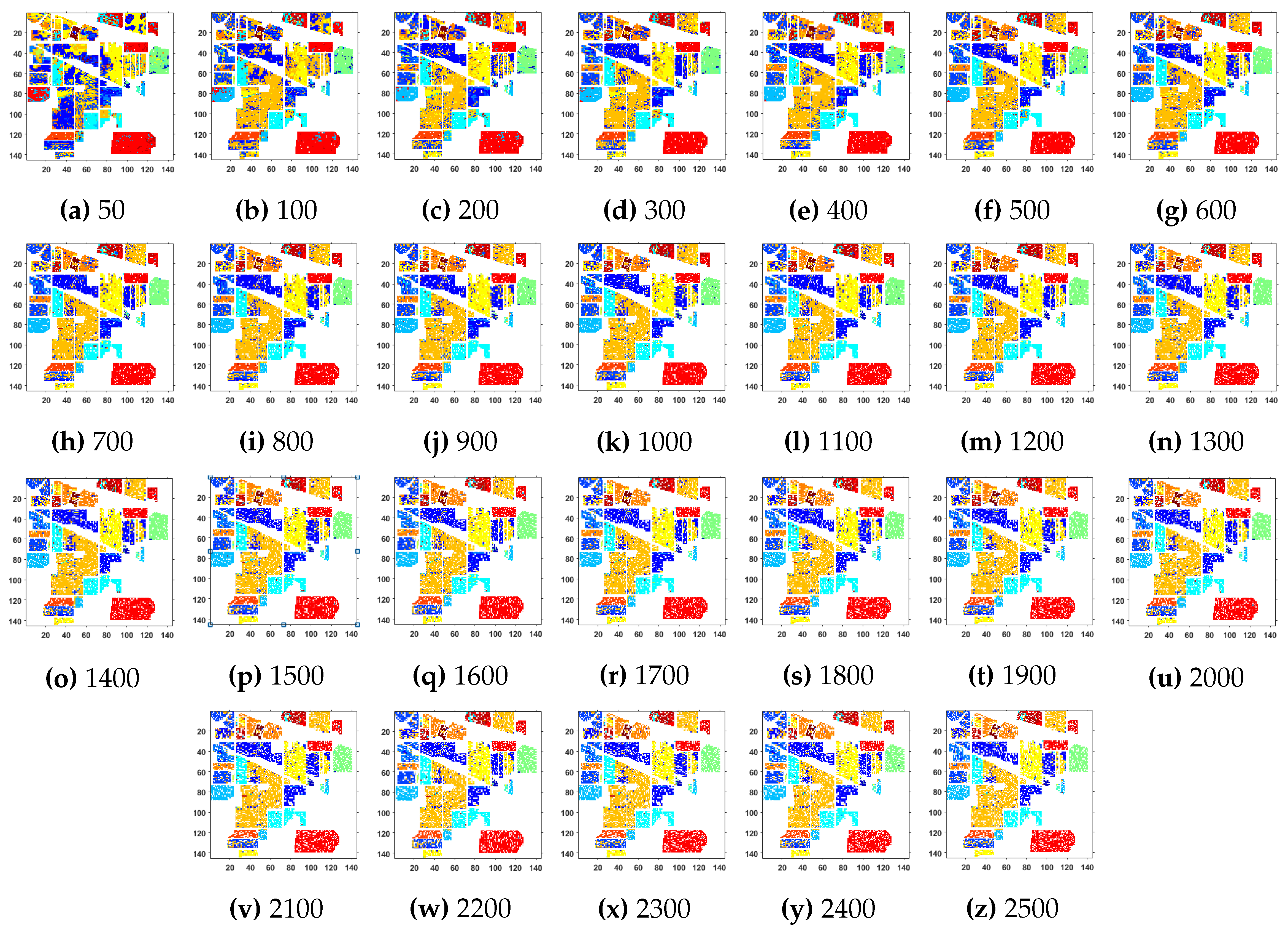
4.2. Experimental Results on Indian Pines Dataset

Indian Pines dataset was collected over northwestern Indiana’s test site, Indian Pines, by AVIRIS sensor and comprises of $145\times 145$ pixels and 224 bands in the wavelength range 0.4–2.5 ×${10}^{-6}$ m. This dataset consists of two-thirds agriculture area and one-third forest or other naturally evergreen vegetation. A railway line, two dual-lane highways, low-density building and housing and small roads are also part of this dataset. Furthermore, some corps in the early stages of their growth is also present with approximately less than $5\%$ of total coverage. The ground truth is comprised of a total of 16 classes but they all are not mutually exclusive. The number of spectral bands is reduced to 200 from 224, by removing the water absorption bands.

Further details about Indian Pines dataset can be found at [44].

Table 2. five-fold cross-validation based statistical and accuracies analysis for MLR-LORSAL Classifier with different Sample Selection methods. The highest values are in bold face.

Metric	MI	BT	MBT	Fuzziness
Overall Accuracy	0.80 ± 0.17	0.81 ± 0.17	0.77 ± 0.14	0.81 ± 0.14
$\mathbf{\kappa }$	0.78 ± 0.19	0.79 ± 0.19	0.74 ± 0.16	0.80 ± 0.16
Recall	0.92 ± 0.01	0.81 ± 0.02	0.69 ± 0.03	0.93 ± 0.02
Precision	0.95 ± 0.01	0.80 ± 0.02	0.63 ± 0.03	0.92 ± 0.02
F1-Score	0.94 ± 0.01	0.79 ± 0.01	0.66 ± 0.03	0.92 ± 0.02

and Figure 2 presents the accuracies for different Classifiers as well as with different sample selection methods. From comparative results, one can see that fuzziness together with MLR-LORSAL classifier works better as compared to the other sample selection and classification methods. We also presents the Indiana Pines predicted geographical maps (classification maps) in Figure 3. These geographical locations of each predicted class label validate the superiority of our proposed pipeline. Figure 3 shows the complete performance assessment on experimental results with profound improvement. As shown in the figure, the classification maps generated by adopting the proposed pipeline are less noisy and more accurate.

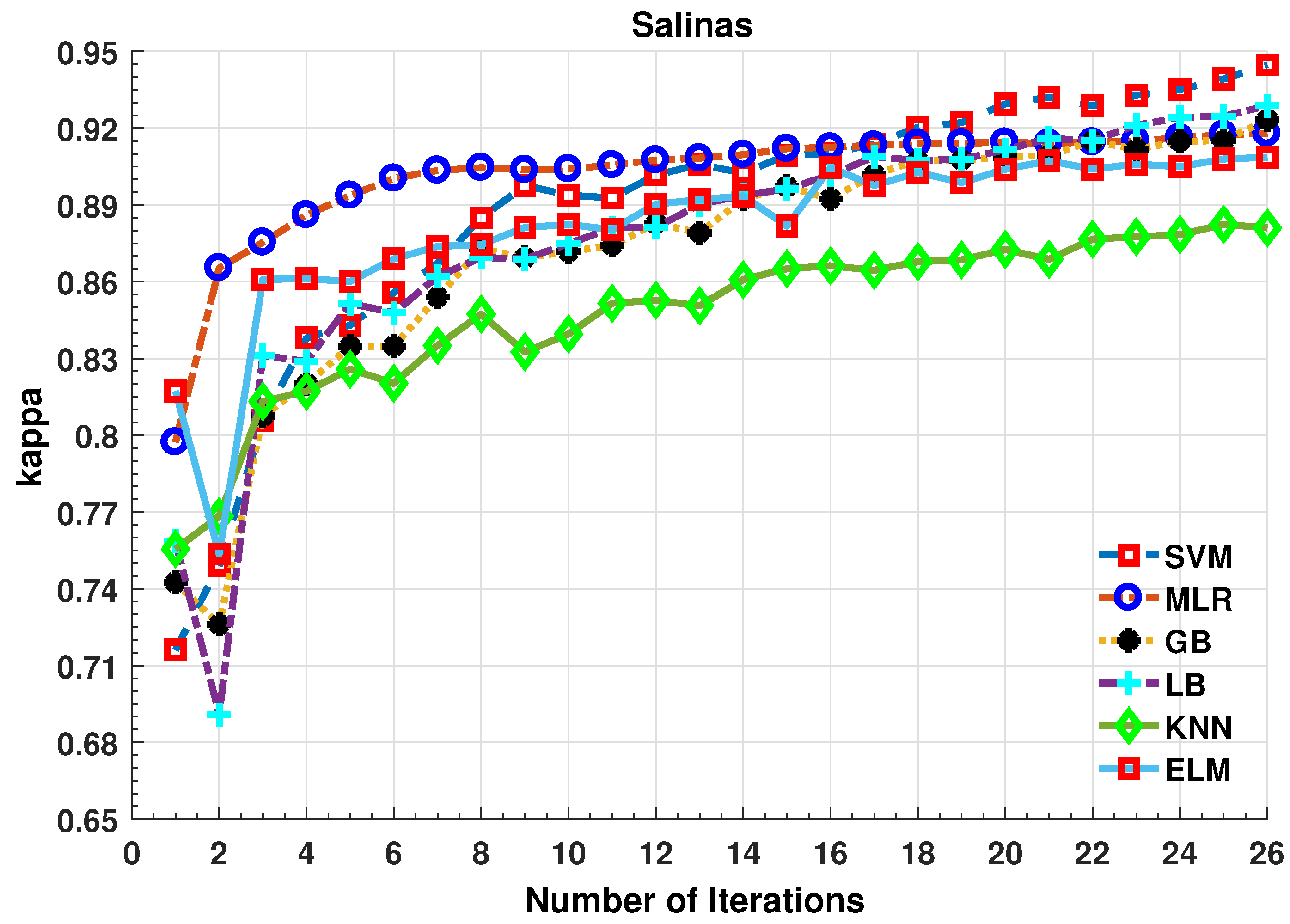
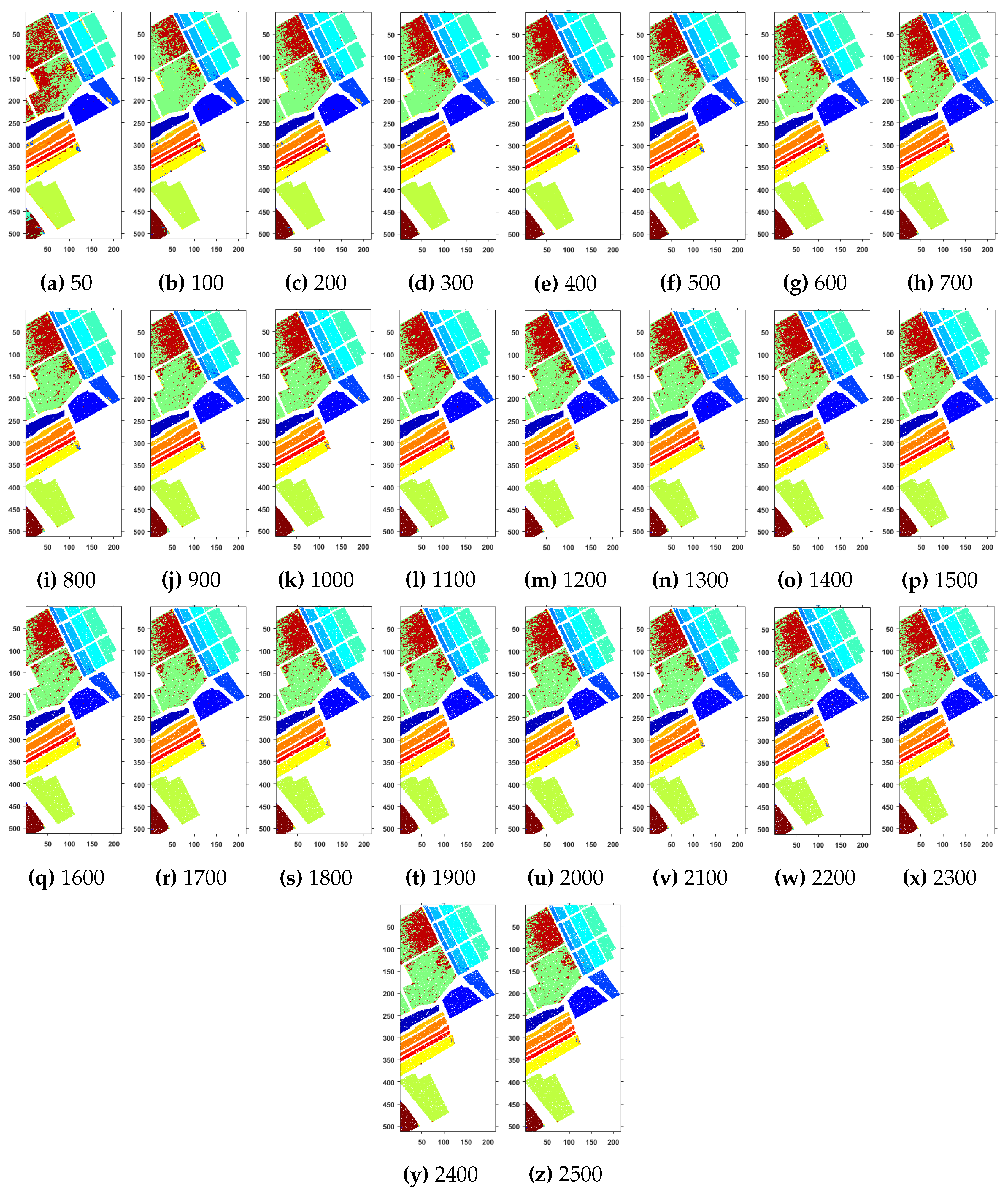
4.3. Experimental Results on Salinas

The Salinas full scene was gathered over Salinas Valley California, through AVIRIS sensor. It comprises $512\times 217$ pixels per band and a total of 244 bands with a $3.7$ m spatial resolution. It consists of vineyard fields, vegetables and bare soils and contains sixteen classes. Few water absorption bands (108–112, 154–167 and 224) are removed from the dataset before analysis. Further details about the dataset can be found at [44].

Further details about Salinas dataset can be found at [44].

Table 3. five-fold cross-validation based statistical and accuracies analysis for MLR-LORSAL Classifier with different Sample Selection methods. The highest values are in bold face.

Metric	MI	BT	MBT	Fuzziness
Overall Accuracy	0.90 ± 0.06	0.91 ± 0.06	0.88 ± 0.05	0.90 ± 0.05
$\mathbf{\kappa }$	0.88 ± 0.06	0.90 ± 0.06	0.87 ± 0.05	0.88 ± 0.05
Recall	0.94 ± 0.01	0.95 ± 0.01	0.94 ± 0.01	0.94 ± 0.01
Precision	0.94 ± 0.01	0.94 ± 0.01	0.94 ± 0.01	0.93 ± 0.01
F1-Score	0.94 ± 0.01	0.94 ± 0.01	0.94 ± 0.01	0.93 ± 0.01

and Figure 4 presents the accuracies for different classifiers as well as with different sample selection methods. From comparative results, one can see that fuzziness together with MLR-LORSAL classifier works better as compared to the other sample selection and classification methods. We also presents the Salinas predicted geographical maps (classification maps) in Figure 5. These geographical locations of each predicted class label validate the superiority of our proposed pipeline. Figure 5 show the complete performance assessment on experimental results with profound improvement. As shown in the figure, the classification maps generated by adopting the proposed pipeline are less noisy and more accurate.

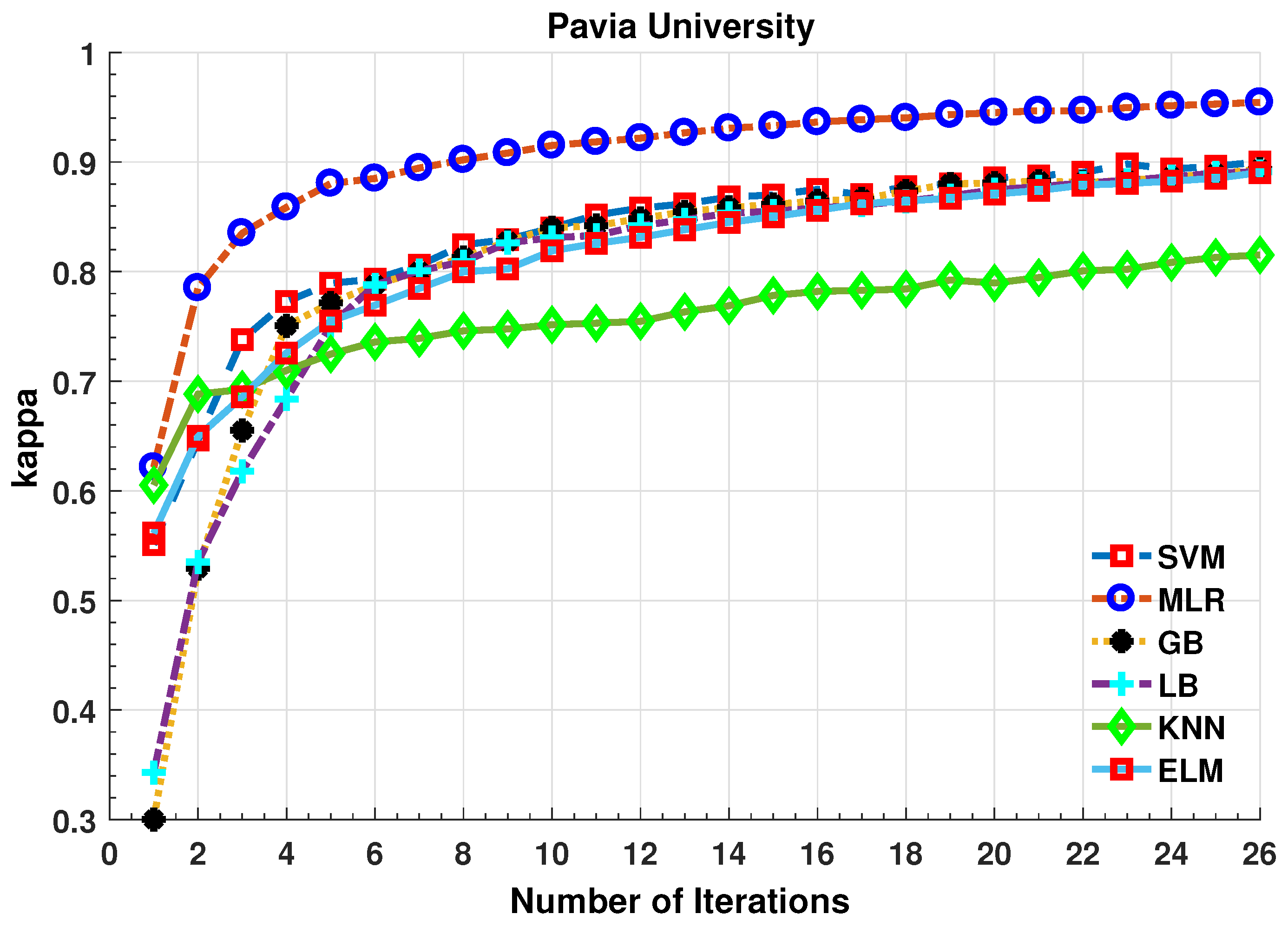
4.4. Experimental Results on Pavia University

Pavia University dataset is gathered over Pavia in northern Italy through ROSIS optical sensor during a flight campaign. It consists of $610\times 610$ pixels and 103 spectral bands with a spatial resolution of $1.3$ m. Some samples in this dataset provide no information and are removed before analysis.

Further details about Pavia University dataset can be found at [44].

Table 4. five-fold cross-validation based statistical and accuracies analysis for MLR-LORSAL Classifier with different Sample Selection methods. The highest values are in bold face.

Metric	MI	BT	MBT	Fuzziness
Overall Accuracy	0.85 ± 0.13	0.88 ± 0.13	0.86 ± 0.12	0.87 ± 0.13
$\mathbf{\kappa }$	0.81 ± 0.16	0.84 ± 0.16	0.82 ± 0.14	0.84 ± 0.15
Recall	0.86 ± 0.02	0.88 ± 0.02	0.88 ± 0.02	0.87 ± 0.02
Precision	0.85 ± 0.03	0.88 ± 0.02	0.86 ± 0.03	0.87 ± 0.03
F1-Score	0.85 ± 0.02	0.87 ± 0.02	0.86 ± 0.02	0.86 ± 0.02

and Figure 6 presents the accuracies for different classifiers as well as with different sample selection methods. From comparative results, one can see that fuzziness together with MLR-LORSAL classifier works better as compared to the other sample selection and classification methods. We also presents the Salinas predicted geographical maps (classification maps) in Figure 7. These geographical locations of each predicted class label validate the superiority of our proposed pipeline. Figure 7 shows the complete performance assessment on experimental results with profound improvement. As shown in the figure, the classification maps generated by adopting the proposed pipeline are less noisy and more accurate.

4.5. Results Discussion

In all the above-shown experiments, the performance of the proposed pipeline is being evaluated using a set of experiments i.e., first, we analyze several sample selection methods for MLR-LORSAL classifier. Later this work compared several classifiers for the same sample selection methods. In all these experiments, the size of the training set is fixed to the maximum of 50 samples randomly selected from all the classes while giving equal representation to each class. In each iteration, 100 new samples are selected based on sample selection method and their spatial locations i.e., the newly selected samples should not be spatially close to the previously selected samples. This phenomenon significantly helps to limit the redundancy factor among the training samples.

The experiments are repeated on more complicated and nested region datasets such as Pavia University dataset. The number of training samples selected in each iteration is shown in the above figures. Based on the results, one can conclude that the fuzziness-based sample selection method is a competitive process that slightly worked better than other well-know sample selection methods. One can conclude from the results shown in Table 2, Table 3 and Table 4 and Figure 2, Figure 3, Figure 4, Figure 5, Figure 6 and Figure 7 that all the sample selection methods performed well, however, BT and Fuzziness-based samples boost the accuracy for MLR-LORSAL classifier followed by MI. From several observations with a different number of training samples, there is a slight improvement in performance using MBT however, fuzziness and BT improve the generalization in impressive fashion. Fuzziness-based sample selection process works better due to the fact that these samples are usually close to the classification boundary.

This work started evaluating the hypotheses with a 50 number of randomly selected samples; it is a well-known fact that the spectral information-based randomly adding samples back to the training set does not increase the accuracy as desired. Therefore, this work explicitly fuses the spatial information while considering the new samples for a training set which significantly boosts the accuracy and generalization performance of a classifier. Furthermore, this work also validates the sufficient number of samples required to train a classifier; i.e., $500-1000$ samples are more than enough to train a classifier to produce an acceptable accuracy for HSI classification tasks.

5. Conclusions

A novel AL for HSI datasets has been explored in this study to overcome the limitations of randomness using spatial–spectral information with predefined dual stopping criteria using a fuzziness-based MLR-LORSAL classifier. Extensive comparisons with state-of-the-art sample selection and classification methods have been carried out. Furthermore, several statistical tests were also considered to validate the claims that the fuzziness-based MLR-LORSAL classifiers outperformed other state-of-the-art classifiers. In short, this work investigated different sample selection techniques and classifiers to properly generalize them to the classification of remotely sensed HSIs with multiclass problems. The experimental results on three benchmark hyperspectral datasets reveal that the proposed pipeline significantly increases the classification accuracy and generalization performance.

References

1. Ahmad, M.; Shabbir, S.; Oliva, D.; Mazzara, M.; Distefano, S. Spatial-prior Generalized Fuzziness Extreme Learning Machine Autoencoder-based Active Learning for Hyperspectral Image Classification. Optik-Int. J. Light Electron Opt. 2020, 206, 163712. [Google Scholar] [CrossRef]
2. Ahmad, M.; Haq, I.U. Linear Unmixing and Target Detection of Hyperspectral Imagery Using OSP. In Proceedings of the International Conference on Modeling, Simulation and Control, Singapore, 25–27 January 2011; pp. 179–183. [Google Scholar]
3. Banerjee, B.P.; Raval, S.; Cullen, P.J. UAV-hyperspectral imaging of spectrally complex environments. Int. J. Remote Sens. 2020, 41, 4136–4159. [Google Scholar] [CrossRef]
4. Jia, B.; Wang, W.; Ni, X.; Lawrence, K.C.; Zhuang, H.; Yoon, S.C.; Gao, Z. Essential processing methods of hyperspectral images of agricultural and food products. Chemom. Intell. Lab. Syst. 2020, 198, 103936. [Google Scholar] [CrossRef]
5. Koz, A. Ground-Based Hyperspectral Image Surveillance Systems for Explosive Detection: Part II—Radiance to Reflectance Conversions. IEEE J. Sel. Top. Appl. Earth Obs. Remote Sens. 2019, 12, 4754–4765. [Google Scholar] [CrossRef]
6. Ahmad, M.; Khan, A.; Khan, A.M.; Mazzara, M.; Distefano, S.; Sohaib, A.; Nibouche, O. Spatial Prior Fuzziness Pool-Based Interactive Classification of Hyperspectral Images. Remote Sens. 2019, 11, 1136. [Google Scholar] [CrossRef] [Green Version]
7. Erickson, Z.; Luskey, N.; Chernova, S.; Kemp, C.C. Classification of Household Materials via Spectroscopy. IEEE Robot. Autom. Lett. 2019, 4, 700–707. [Google Scholar] [CrossRef] [Green Version]
8. Jiang, Y.; Snider, J.L.; Li, C.; Rains, G.C.; Paterson, A.H. Ground Based Hyperspectral Imaging to Characterize Canopy-Level Photosynthetic Activities. Remote Sens. 2020, 12, 315. [Google Scholar] [CrossRef] [Green Version]
9. Ahmad, M.; Khan, A.M.; Mazzara, M.; Distefano, S. Multi-layer Extreme Learning Machine-based Autoencoder for Hyperspectral Image Classification. In Proceedings of the 14th International Conference on Computer Vision Theory and Applications (VISAPP’19), Prague, Czech Republic, 25–27 February 2019; pp. 25–27. [Google Scholar]
10. Alcolea, A.; Paoletti, M.E.; Haut, J.M.; Resano, J.; Plaza, A. Inference in Supervised Spectral Classifiers for On-Board Hyperspectral Imaging: An Overview. Remote Sens. 2020, 12, 534. [Google Scholar] [CrossRef] [Green Version]
11. Wang, Y.; Yu, W.; Fang, Z. Multiple Kernel-Based SVM Classification of Hyperspectral Images by Combining Spectral, Spatial, and Semantic Information. Remote Sens. 2020, 12, 120. [Google Scholar] [CrossRef] [Green Version]
12. Vincent, F.; Besson, O. One-Step Generalized Likelihood Ratio Test for Subpixel Target Detection in Hyperspectral Imaging. IEEE Trans. Geosci. Remote Sens. 2020, 58, 4479–4489. [Google Scholar] [CrossRef] [Green Version]
13. Su, H.; Yu, Y.; Du, Q.; Du, P. Ensemble Learning for Hyperspectral Image Classification Using Tangent Collaborative Representation. IEEE Trans. Geosci. Remote Sens. 2020, 58, 3778–3790. [Google Scholar] [CrossRef]
14. Pan, B.; Shi, Z.; Xu, X. Hierarchical guidance filtering-based ensemble classification for hyperspectral images. IEEE Trans. Geosci. Remote Sens. 2017, 55, 4177–4189. [Google Scholar] [CrossRef]
15. Alshurafa, N.I.; Katsaggelos, A.K.; Cossairt, O.S. Hyperspectral Imaging Sensor. U.S. Patent App. 16/492,214, 1 February 2020. [Google Scholar]
16. Xia, J.; Du, P.; He, X.; Chanussot, J. Hyperspectral remote sensing image classification based on rotation forest. IEEE Geosci. Remote Sens. Lett. 2013, 11, 239–243. [Google Scholar] [CrossRef] [Green Version]
17. Safari, K.; Prasad, S.; Labate, D. A Multiscale Deep Learning Approach for High-Resolution Hyperspectral Image Classification. IEEE Geosci. Remote Sens. Lett. 2020. [Google Scholar] [CrossRef]
18. Song, A.; Kim, Y. Deep learning-based hyperspectral image classification with application to environmental geographic information systems. Korean J. Remote Sens. 2017, 33, 1061–1073. [Google Scholar]
19. Ahmad, M. A Fast 3D CNN for Hyperspectral Image Classification. arXiv 2020, arXiv:2004.14152. [Google Scholar]
20. Liu, B.; Yu, X.; Yu, A.; Wan, G. Deep convolutional recurrent neural network with transfer learning for hyperspectral image classification. J. Appl. Remote Sens. 2018, 12, 1–17. [Google Scholar] [CrossRef]
21. Yang, J.; Zhao, Y.; Chan, J.C. Learning and Transferring Deep Joint Spectral–Spatial Features for Hyperspectral Classification. IEEE Trans. Geosci. Remote Sens. 2017, 55, 4729–4742. [Google Scholar] [CrossRef]
22. Ma, J.; Xiao, B.; Deng, C. Graph based semi-supervised classification with probabilistic nearest neighbors. Pattern Recognit. Lett. 2020, 133, 94–101. [Google Scholar] [CrossRef]
23. Ahmad, M. Fuzziness-based Spatial-Spectral Class Discriminant Information Preserving Active Learning for Hyperspectral Image Classification. arXiv 2020, arXiv:2005.14236. [Google Scholar]
24. Hughes, G. On the mean accuracy of statistical pattern recognizers. IEEE Trans. Inf. Theory 1968, 14, 55–63. [Google Scholar] [CrossRef] [Green Version]
25. Ahmad, M.; Protasov, S.; Khan, A.M.; Hussain, R.; Khattak, A.M.; Khan, W.A. Fuzziness-based active learning framework to enhance hyperspectral image classification performance for discriminative and generative classifiers. PLoS ONE 2018, 13, e0188996. [Google Scholar] [CrossRef] [PubMed]
26. Bovolo, F.; Bruzzone, L.; Carlin, L. A novel technique for subpixel image classification based on support vector machine. IEEE Trans. Image Process. 2010, 19, 2983–2999. [Google Scholar] [CrossRef] [PubMed]
27. Persello, C.; Bruzzone, L. Active and semisupervised learning for the classification of remote sensing images. IEEE Trans. Geosci. Remote Sens. 2014, 52, 6937–6956. [Google Scholar] [CrossRef]
28. Cao, X.; Yao, J.; Xu, Z.; Meng, D. Hyperspectral Image Classification With Convolutional Neural Network and Active Learning. IEEE Trans. Geosci. Remote Sens. 2020, 58, 4604–4616. [Google Scholar] [CrossRef]
29. Shahshahani, B.M.; Landgrebe, D.A. The effect of unlabeled samples in reducing the small sample size problem and mitigating the Hughes phenomenon. IEEE Trans. Geosci. Remote Sens. 1994, 32, 1087–1095. [Google Scholar] [CrossRef] [Green Version]
30. Yang, L.; Yang, S.; Jin, P.; Zhang, R. Semi-supervised hyperspectral image classification using spatio-spectral Laplacian support vector machine. IEEE Geosci. Remote Sens. Lett. 2013, 11, 651–655. [Google Scholar] [CrossRef]
31. Fang, L.; Zhao, W.; He, N.; Zhu, J. Multiscale CNNs Ensemble Based Self-Learning for Hyperspectral Image Classification. IEEE Geosci. Remote Sens. Lett. 2020. [Google Scholar] [CrossRef]
32. Melville, P.; Mooney, R.J. Diverse ensembles for active learning. In Proceedings of the Twenty-First International Conference on Machine Learning; ACM: New York, NY, USA, 2004; p. 74. [Google Scholar]
33. Jamshidpour, N.; Safari, A.; Homayouni, S. A GA-Based Multi-View, Multi-Learner Active Learning Framework for Hyperspectral Image Classification. Remote Sens. 2020, 12, 297. [Google Scholar] [CrossRef] [Green Version]
34. Zhou, Z.H.; Li, M. Tri-training: Exploiting unlabeled data using three classifiers. IEEE Trans. Knowl. Data Eng. 2005, 17, 1529–1541. [Google Scholar] [CrossRef] [Green Version]
35. Ahmad, M.; Khan, A.M.; Hussain, R. Graph-based spatial–spectral feature learning for hyperspectral image classification. IET Image Process. 2017, 11, 1310–1316. [Google Scholar] [CrossRef]
36. Yu, H.; Yang, X.; Zheng, S.; Sun, C. Active learning from imbalanced data: A solution of online weighted extreme learning machine. IEEE Trans. Neural Netw. Learn. Syst. 2018, 30, 1088–1103. [Google Scholar] [CrossRef] [PubMed]
37. Li, J.; Bioucas-Dias, J.M.; Plaza, A. Spectral–spatial classification of hyperspectral data using loopy belief propagation and active learning. IEEE Trans. Geosci. Remote Sens. 2012, 51, 844–856. [Google Scholar] [CrossRef]
38. Tuia, D.; Ratle, F.; Pacifici, F.; Kanevski, M.F.; Emery, W.J. Active learning methods for remote sensing image classification. IEEE Trans. Geosci. Remote Sens. 2009, 47, 2218–2232. [Google Scholar] [CrossRef]
39. Li, J.; Bioucas-Dias, J.M.; Plaza, A. Hyperspectral image segmentation using a new Bayesian approach with active learning. IEEE Trans. Geosci. Remote Sens. 2011, 49, 3947–3960. [Google Scholar] [CrossRef] [Green Version]
40. Yu, H.; Sun, C.; Yang, W.; Yang, X.; Zuo, X. AL-ELM: One uncertainty-based active learning algorithm using extreme learning machine. Neurocomputing 2015, 166, 140–150. [Google Scholar] [CrossRef]
41. Böhning, D. Multinomial logistic regression algorithm. Ann. Inst. Stat. Math. 1992, 44, 197–200. [Google Scholar] [CrossRef]
42. Camps-Valls, G.; Bruzzone, L. Kernel-based methods for hyperspectral image classification. IEEE Trans. Geosci. Remote Sens. 2005, 43, 1351–1362. [Google Scholar] [CrossRef]
43. De Luca, A.; Termini, S. A definition of a nonprobabilistic entropy in the setting of fuzzy sets theory. Inf. Control 1972, 20, 301–312. [Google Scholar] [CrossRef] [Green Version]
44. Hyperspectral Datasets Description. 2020. Available online: http://www.ehu.eus/ccwintco/index.php/Hyperspectral_Remote_Sensing_Scenes (accessed on 12 January 2020).
45. Yang, J.; Yu, H.; Yang, X.; Zuo, X. Imbalanced extreme learning machine based on probability density estimation. In International Workshop on Multi-Disciplinary Trends in Artificial Intelligence; Springer: Fuzhou, China, 2015; pp. 160–167. [Google Scholar]
46. Liu, W.; Yang, J.; Li, P.; Han, Y.; Zhao, J.; Shi, H. A novel object-based supervised classification method with active learning and random forest for PolSAR imagery. Remote Sens. 2018, 10, 1092. [Google Scholar] [CrossRef] [Green Version]
Figure 1. Computational Time for MLR-LORSAL Classifier for all Query Functions for three different datasets.
Applsci 10 04739 g001
Figure 2. Comparative Results for Several Classifiers with respect to the κ accuracy for different number of training samples ([50:100:2500]) selected in each iteration.
Applsci 10 04739 g002
Figure 3. Geographical Locations for Predicted Test Labels of Indian Pines Dataset with respect to the number of training samples, ranging from (a) 50 samples to (z) 2500 samples. The total number of samples in the data are 21,025.
Applsci 10 04739 g003
Figure 4. Comparative Results for Several Classifiers with respect to the κ accuracy for different number of training samples ([50:100:2500]) selected in each iteration.
Applsci 10 04739 g004
Figure 5. Geographical Locations for Predicted Test Labels of Indian Pines Dataset with respect to the number of training samples, ranging from (a) 50 samples to (z) 2500 samples. The Total Number of Samples are 111,104.
Applsci 10 04739 g005
Figure 6. Comparative Results for Several Classifiers with respect to the κ accuracy for different number of training samples ([50:100:2500]) selected in each iteration.
Applsci 10 04739 g006
Figure 7. Geographical Locations for Predicted Test Labels of Indian Pines Dataset with respect to the number of training samples, ranging from (a) 50 samples to (z) 2500 samples. The Total Number of Samples are 372 , 100 .
Applsci 10 04739 g007