Abstract
In the current fatigue life calculation theory, the most commonly used method is the frequency domain method. However, most of the frequency domain fatigue life prediction models do not indicate the scope of the application of the spectral width parameter. Different frequency domain methods have strict applicability to the spectral width parameter, and improper model selection will lead significant error. Therefore, it is particularly important to determine the scope of application of the spectral width parameter for different frequency-domain methods. This paper firstly introduces the current frequency domain methods, then simulates the analogue spectrum and selects three materials for comparison in the different frequency-domain methods. By analyzing and comparing the results of random fatigue life and relative error results, the application of different frequency-domain methods is obtained, and random vibration simulation verification is carried out with the practical engineering example, which can provide a reference for the selection of life prediction models.
1. Introduction
Fatigue failure is one of the most important failure modes in engineering structures, and more than 85% of the structural failures are fatigue failures. Generally, the fatigue load can be divided into three types: constant amplitude fatigue, variable amplitude fatigue, and random fatigue [1]. Among them, constant amplitude fatigue and variable amplitude fatigue have been studied in most fields, and the theory and design are relatively perfect [2]. However, there is little research in the field of random fatigue. Most civil structures inevitably bear random loads, such as wind loads, pedestrian-vehicle loads, etc., so the study of random fatigue in the field of civil engineering is also very necessary.
Fatigue life estimation is mainly obtained through the cumulative damage criterion and the S-N curve of the material. For random fatigue, life estimation methods are divided into the time-domain method and frequency-domain method [3]. The time-domain method is to analyze the time history of the response stress of the structure, and obtain the amplitude, mean value and cycle times of the response stress by a certain cycle counting method, and then calculate the fatigue damage and life of the structure by combining with the appropriate cumulative damage theory [4] and S-N curve of the material [5]. In this method, many scholars have proposed different cycle counting methods for the response stress time history, and the rain flow counting method proposed by Matsuishi and Endo [5] is considered to be the most accurate cycle counting method in fatigue damage and fatigue life estimation [6,7,8]. The rain flow solution is also usually used as an accurate solution or a standard solution in random fatigue life analysis. However, the time-domain method has a large amount of calculation, the time-history curve is difficult to obtain, and the operability is not good in engineering applications [9]. Therefore, in order to avoid various shortcomings of the time-domain method, the frequency-domain method has been developed to simplify the calculation of random fatigue damage and life. The frequency domain refers to another coordinate system used to describe the frequency characteristic of random processes [10]. By performing a fast Fourier transform on the time domain signal, the various frequency components of the random process are separated to obtain the power spectral density and describe the characteristic with its corresponding spectral parameters. This is the basic idea of the frequency domain method [11]. The power spectral density is the “power” in a unit frequency band. Mathematically, the area enclosed by the power spectral density curve and the coordinate axis is equal to the mean square value of the signal [12,13]. The power spectral density can be divided into a broadband random process and a narrow-band random process according to their different spectral types [14,15].
Many scholars have conducted a lot of research on different frequency domain methods. Matjaž Mršnik, Janko Slavič [16], and others compared the above common methods through the measured data, and found that Tove–Benasciutti, Zhao–Baker, and Dirlik methods have high accuracy, applicability, and can be used as the recommended method for fatigue life estimation. Braccesi [17] proposed a new original index to evaluate the reliability of the frequency domain method for the stochastic process of double peak stress. Wang and Shang [18] performed fatigue testing on tensile shear spot welding specimens, and established a life prediction model for spot welding under random load through damage mechanics. Wang Mingzhu [19] studied the influence of frequency on the fatigue life curve of metal materials, and proposed a fatigue S-N curve model of metal materials. Zhen Gao and Torgeir Moan [20] proposed the fatigue life estimation method for the three-peak stochastic process based on the theory of the two-peak approximation method, and extended it to the generalized broadband stochastic process. Benasciutti [21,22] proposed a new method to predict fatigue life in frequency domain, and pointed out that in the wide-band random process, the narrow-band distribution method and its improved method will produce some conservative results, and the T–B method and Dirlik method are superior to other frequency-domain methods.
When the load frequency range of the structure changes, the frequency range of the structural response will also change, resulting in the change of the spectrum width parameter of the response spectrum. At this time, for random fatigue damage and life calculation, the choice of the life prediction model is particularly important for the adaptability of different spectral width parameters. In the calculation of random fatigue life, the most commonly used method is the frequency domain method. At present, most frequency-domain fatigue life prediction models only specify whether they are applicable to narrowband or wideband, and do not indicate the specific application range of the spectrum width parameter. Different frequency domain methods have more stringent applicability to spectral width parameters, rather than universality. Improper model selection will lead to large errors. Different frequency domain methods have more stringent applicability to spectral width parameters, rather than universality. Improper model selection will lead to large errors. At present, there is no clear boundary between the narrowband and wideband. Thus far, the range of narrowband and wideband spectral width parameters has not been clearly defined [23]. Therefore, it is more difficult to choose the appropriate fatigue life prediction model. At this time, it is more important to determine the application range of different spectrum width parameters for different frequency-domain methods. This article mainly studies the applicability of several common frequency-domain methods to different spectral width parameters.
2. Common Frequency Domain Methods
In frequency-domain method, autocorrelation function is generally used to describe the time-varying characteristic of the stationary random process. The power spectral density describes the stationary process in the frequency domain and can express the energy distribution of the random process [24].
Theoretically, the autocorrelation function and power spectral density conform to the Wiener–Sinchin theorem, as shown in Equation (1):
The power spectral density of random process X (t) can be divided into unilateral power spectral density and bilateral power spectral density. In practice, the frequency is always greater than zero, so the one-sided power spectral density is defined in Equation (2) as:
Statistical moments are numerical characteristics describing the probability density. Similarly, scholars introduce spectral moments to describe the numerical characteristics of the spectral density of random processes. According to ω = 2πf, the spectral moment mi of the stationary random process X (t) is expressed in Equation (3) as the unilateral power spectral density:
In general, the irregular factor γ can be introduced to determine whether a stationary random process X (t) conforms to a narrow-band process or a wide-band process:
In Equation (4), when γ→1, the random process tends to narrow-band random process; when γ→0, the random process tends to a broadband random process.
The bandwidth parameter ε is often introduced in engineering to describe the bandwidth of random processes:
In Equation (5), when ε→0, the random process tends to narrow-band random process; when ε→1, the random process tends to a broadband random process.
If a Gaussian random process is known, the peak expected rate vp and positive slope crossing expected value v0 per unit time can be obtained based on its power spectral density, as shown in Equation (6):
According to different statistical parameters, the frequency domain method can be divided into two types: the peak distribution method and the amplitude distribution method. The peak distribution method approximates the distribution of peaks to calculate the fatigue damage of the structure, which is more suitable for the broadband stable Gaussian process. The amplitude distribution method is to obtain the probability density distribution function of the amplitude of the rain flow in response to stress through experiment or simulation, and then calculate the fatigue life by combining with the fatigue damage theory. The random process can be divided into narrowband approximation and wideband correction according to the bandwidth characteristics. Since the amplitude distribution method is simpler, intuitive, and convenient for application, it has been widely used in the engineering field. The frequency domain methods adopted in this paper are all based on the amplitude distribution method.
For the stationary Gaussian random process, there are many methods to estimate the damage of the structure under random load. For narrow-band stationary Gaussian stochastic processes, Bendat proposed to use Rayleigh distribution to describe the probability density distribution of rain flow amplitude, and it has been confirmed [25,26]. For the broadband stable Gaussian random process, due to the large difference in the distribution of rain flow amplitude, there is no unified fatigue life prediction model for academic analysis, but many scholars have proposed many different frequency domain empirical formulas. In 1980, after studying the power spectral density of different shapes, Wirsching-Light [2] proposed a correction factor to correct the fatigue damage calculated by the narrow-band method. Benasciutti and Tovo [27] proposed a new spectral width parameter α0.75 through a large number of numerical simulations, and used the correction factor to improve the narrow-band method, so this method is also called the α0.75 method. The Tovo–Benasciutti [28] method divides the broadband stochastic process into two parts, high frequency and low frequency, and treats them as narrow-band stochastic processes. Then the rain-fatigue damage of the original stochastic process is equivalent to these two narrow-band spectral fatigue damage superposition. Dirlik [29,30], Zhao and Baker [31], etc., proposed a different stress amplitude probability density function model by combining known probability density distribution functions. Ortiz and Chen [32] proposed new correction parameters by studying the Rayleigh distribution under different spectral widths. Larsen and Lutes [33] obtained a single-moment method suitable for estimating the random fatigue life of the bimodal spectrum through a large number of numerical simulations and rain flow amplitude analysis. The Nakagami method [34] believes that the Nakagami distribution model can not only accurately simulate the shape of the rain flow amplitude probability density distribution model, but also can make a good approximation of its tail compared to other distribution models.
- Narrowband method (NB).
For the narrow-band random process, Bendat [25] proposed to describe the probability density distribution of the rain-flow amplitude with the Rayleigh distribution. He assumed that each cycle of the rain-flow amplitude of the narrow-band random process was completely symmetric, that is, the equivalent peak-valley cycle. The specific functional expression is shown in Equation (7):
where is the mean stress square value of the random process, and S is the stress amplitude.
Since the number of mean positive crossing and the number of peak occurrence in unit time of the narrow-band random process are equal, the fatigue damage formula of the structure in unit time in this case is transformed into:
In Equation (8), f(S) is the N value in the S-N curve.
The Rayleigh distribution has higher applicability to the narrow-band random process, but it has poor applicability to the wide-band random process, because the probability of occurrence of stress cycles in the low-stress region in the wide-band random process will be higher than that of the narrow-band process. At this time, if the narrow-band method is used to estimate the fatigue damage and fatigue life, it is likely to overestimate and obtain a very conservative life value, which will have a greater impact on engineering applications.
- 2.
- Wirsching-Light method (WL).
In the Wirsching-Light method, the fatigue damage per unit time of the structure is shown in Equation (9):
where ρWL is related to the spectral width parameter ε and the slope α of the S-N curve, the specific expression is shown in Equation (10):
The parameters A and B are both related to the slope value α. The specific formula is:
- 3.
- α0.75 method (AL).
In the α0.75 method, the structural fatigue damage per unit time can be calculated is shown in Equation (11):
- 4.
- Ortiz and Chen method (OC).
Ortiz and Chen [32] studied the Rayleigh distribution under different spectral width parameters and proposed the following new correction parameter, as shown in Equations (12) and (13):
where k’ = 2.0/k.
The Wirsching-Light method, α0.75 method, and Ortiz and Chen method all proposed to modify the Bendat narrow-band fatigue life estimation with a broadband coefficient, so as to obtain the fatigue life of wideband stochastic process. However, these methods ignore the probability distribution information of stress amplitude and only calculates the fatigue life, which are only applicable to some specific cases.
- 5.
- Tovo–Benasciutti method (TB).
Through extensive research, Tovo–Benasciutti [28] found that the rain damage of the Gaussian process is always bounded, DRFC is between the upper and lower limits of Rayleigh fatigue damage DNB and the damage DRC of the variable range mean counting method, as shown in Equation (14):
Therefore, the rain damage value can be calculated through a certain linear combination, and the weight coefficient b is selected to obtain the structural damage, as shown in Equations (15) and (16):
Therefore:
In Equation (17), for the value of parameter b, there are currently two forms are shown in Equations (18) and (19):
According to the different values of parameter b, the TB method is divided into TB1 and TB2 methods. In the wideband random process, the narrow-band fractional step method and its improvement method can get conservative results, while the T–B method can get more accurate results.
- 6.
- Dirlik method (DI).
The Dirlik method [29,30] is an empirical closed formula that includes an exponential distribution function and two Rayleigh distribution functions. The two distribution functions are linearly combined to simulate the probability density distribution of rain flow amplitude. The specific calculation formula is shown in Equation (20):
where:
It is proved by experiments that Dirlik method is very accurate. However, the main problem of this method lies in that it is an empirical formula completely obtained through experimental simulation without any complete theoretical explanation. In addition, the Dirlik method does not take into account the influence of average stress, so this method is difficult to apply to non-Gaussian random processes with non-zero mean value and large error.
- 7.
- Zhao–Baker method (ZB).
The Zhao–Baker method [31] describes the probability density of the rain flow amplitude through a linear combination of a Rayleigh distribution and a Weibull distribution function. The expression is shown in Equation (21):
The weighting coefficient in Equation (21) is:
The other two parameters , are expressed by the following formula:
The Zhao–Baker method is especially suitable for some specific power spectra.
- 8.
- Single moment method (SM).
In the single moment method, the structural fatigue damage per unit time can be calculated is shown in Equations (22) and (23):
The SM method improves the Rayleigh approximation to some extent, and is suitable for some wideband random processes.
- 9.
- Nakagami method (NK).
The Nakagami method [34] believes that the rain flow amplitude probability density distribution follows the Nakagami distribution, the expression is shown in Equation (22):
where:
3. Analysis of the Change of Spectrum Parameter and Its Influencing Factors
In order to obtain the applicable range of different spectrum width parameters for the different frequency-domain methods, in addition to the change of the spectrum width parameter, the influence of different spectral types and different material parameters must also be considered. Therefore, through the numerical simulation of different simulation spectra and three different materials, the accuracy and applicability of the above 10 methods (including TB method divided into TB1 and TB2) were compared.
3.1. Spectrum Simulation and the Characteristic Parameters
The simulated spectrum taken in this article can be divided into four categories: band-limited white noise spectrum, single-peak spectrum, double-peak spectrum and multi-peak spectrum. In order to control the variables, all the simulated spectra are curves with the same root mean square value of stress and varying spectrum width parameters. The root mean square value of the stress here is taken as 147 MPa, and the spectrum width parameter range is between 0 and 1. In order to cover the spectrum width parameter range as far as possible, Matlab, a commercial mathematics software produced by MathWorks in the United States, is used to adjust the spectrum amplitude and frequency domain range and randomly generate signals with different spectrum width parameters.
- 1.
- Single peak spectrum.
As shown in Figure 1, the single peak spectrum refers to the power spectrum density with only one peak in the whole spectrum line. When the natural frequency of the structure is consistent with or close to the load frequency, a resonance phenomenon will occur, and the response spectrum will generate a peak, so this peak spectrum is also a common response spectrum in engineering. This set of single-peak spectra contains 12 spectral lines, the root mean square stress is 147 MPa, and the spectral width parameters are respectively 0.1875, 0.2657, 0.389, 0.4546, 0.5504, 0.6061, 0.6688, 0.7272, 0.8184, 0.8942, 0.9221, 0.965.
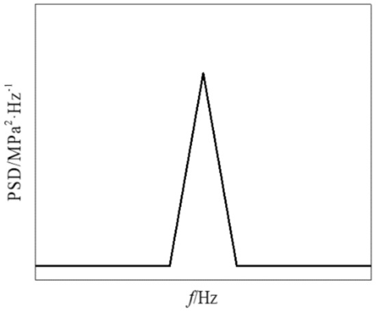
Figure 1.
Single peak simulation spectrum.
- 2.
- Double peak spectrum.
As shown in Figure 2, the double-peak spectrum refers to the entire spectral line that contains only two main frequency peaks. This is also one of the main forms of the dynamic response of engineering structures. When the structure generates two-order resonance, a double-peak response spectrum will be generated. This set of bimodal spectra contains 12 spectral lines with spectral width parameters of 0.1951, 0.2445, 0.3568, 0.4821, 0.5543, 0.6534, 0.7386, 0.8129, 0.8852, 0.9483, 0.9746, 0.9829. Here, we also consider the impact of different background noises on life calculation.
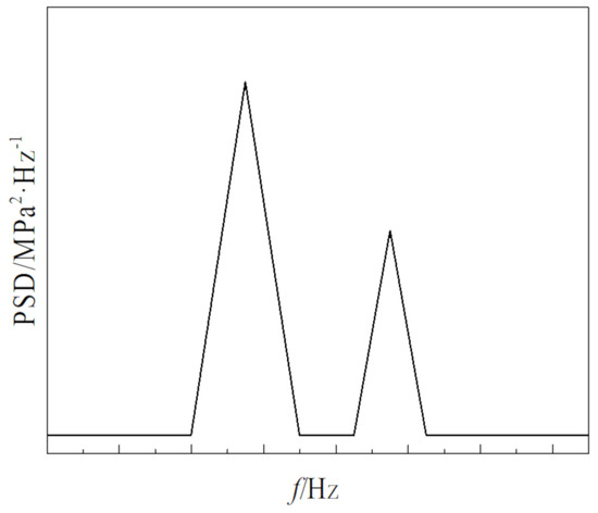
Figure 2.
Double peak simulation spectrum.
- 3.
- Multi-peak spectrum.
As shown in Figure 3, the multi-peak spectrum refers to more than three peaks in the entire spectrum, which is a typical broadband spectrum. When the frequency range of the external load is wide, it can cover the multi-order natural frequency of the structure, then the result will be multi-order resonance, and the multi-peak spectrum will appear in the response spectrum of this case, which is also a common spectrum in structural, mechanical, marine, and aerospace engineering. This group contains a total of 10 sets of spectral lines, the spectral width parameters are: 0.3863, 0.4858, 0.5844, 0.6415, 0.6972, 0.7511, 0.8396, 0.9099, 0.9298, 0.966.
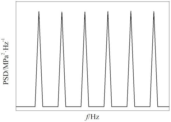
Figure 3.
Multiple peak simulation spectrum.
- 4.
- Band-limited white noise spectrum.
In structural vibration fatigue analysis, the environmental load and stress response of the structure can usually be approximated as a band-limited white noise process or a combination of band-limited white noise processes [35,36], as shown in Figure 4. This group takes a total of 10 sets of band-limited white noise analogue spectrum curves, and changes its spectrum width parameters by changing its frequency range and amplitude. The specific spectral width parameters are: 0.115, 0.18812, 0.2733, 0.3498, 0.4167, 0.474, 0.5225, 0.5631, 0.6248, 0.6667.
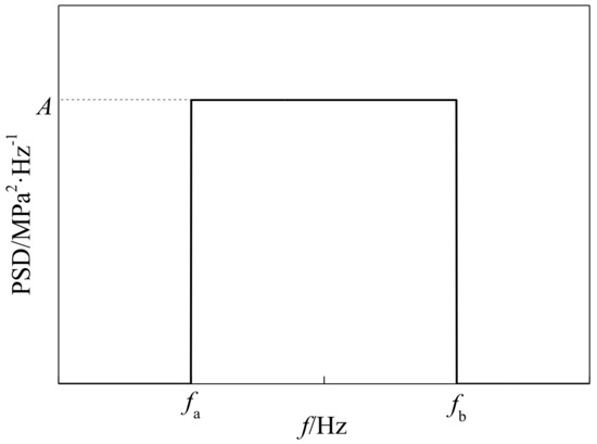
Figure 4.
Band-limited white noise simulation spectrum.
3.2. The Influence of Material Properties
In general, fatigue life curve is used to describe the fatigue performance of materials in engineering, and its power function formula is:
In Equation (25), m and C are material constants. According to Equation (8), when calculating the random fatigue damage in the frequency domain method, the S-N curve of the material also has an important influence. The type of material also affects the accuracy of the random fatigue life in the frequency domain method.
Steel and aluminum alloy are three commonly used materials in engineering. Among them, steel is the most widely used material in most engineering fields, and aluminum alloy is a non-ferrous metal material commonly used in engineering. The functional relationship between the stress amplitude and fatigue life is selected in the form of a power function and three parameters. In order to ensure the reliability of the results, this paper selects one of the three material types for analysis. The slope of the S-N curve affects the calculation accuracy of the frequency domain method, and the slope value of steel and aluminum alloys does not change much, spring steel with a larger slope is selected for analysis. Spring steel is specifically used to make springs and elastic Components of steel. In order to ensure the reliability of the results, in this paper, Q460D steel, LY12 aluminum alloy, and GB/T4657-89 carbon spring steel wire are selected for analysis. The parameters of the three materials are shown in Table 1 [37] to verify the applicability of different frequency-domain methods to different S-N curve models. Su in the table is the ultimate tensile strength.

Table 1.
Material list [37].
3.3. Reference Standard-Time Domain Analysis
In order to obtain the applicability of various frequency-domain methods to different spectral width parameters, it is necessary to compare the estimation results of different frequency-domain methods, which requires obtaining an accurate solution as the comparison standard. In this paper, the life result TRF calculated by the rain current counting method combined with the Miner cumulative damage criterion is selected as the reference standard, so as to achieve the purpose of comparison. Before applying the rain current counting method, since the simulated spectral curve is a frequency domain curve, it needs to be converted into a time history curve. In this paper, the inverse Fourier transform method is selected for time-frequency conversion. Since the simulated spectrum is in the form of power spectral density and does not contain phase information, but for a stationary random process, if it is assumed that its random phase angle is uniformly distributed in the interval [0, 2π] [38], in the end, consistent statistical characteristics can be obtained, and the lifetime results are also equivalent.
In order to obtain a more accurate time-domain result, when applying the time-domain method, not only the influence of rain flow amplitude but also the influence of rain flow mean value must be considered [39]. Therefore, the Goodman equation is added to the time domain method to obtain the rain flow life estimation TRF in Equation (27):
In Equation (26), Su is the ultimate tensile strength, Sa is the stress amplitude, Sm is the average stress, and Sf is the fatigue limit amplitude.
4. Comparative Analysis
The 10 commonly used frequency domain methods described can be divided into two categories. One is the approximate amplitude probability distribution method, including the narrow-band method, Dirlik method, Zhao–Baker method, and Nakagami method. The life density is calculated by simulating the probability density distribution of rain current amplitude. The other type is the correction coefficient method, which uses a correction coefficient to modify the narrowband method to calculate the fatigue life, including the Wirsching-Light method, the Ortiz and Chen method, the Tovo–Benasciutti method (TB1, TB2), and the single-moment method.
4.1. Rainflow Amplitude Distribution
Since the approximate amplitude probability distribution method can intuitively describe the distribution of rain flow amplitude, it is of great theoretical significance to calculate the random fatigue life by the approximate amplitude probability distribution method. This section first studies the applicability of the above four rain flow amplitude probability density distribution functions to different spectral width parameters. Time domain simulation was performed on 44 sets of simulated spectral curves. The rain flow amplitude histogram and the cumulative probability density curve of rain flow amplitude are obtained by the rain flow counting method. By comparing it with four probability density distribution function curves of rain flow amplitude, we can see its applicability to rain flow amplitude. The probability density curves of rain flow amplitude and cumulative probability density curves of the simulated spectrum are shown in Appendix A. In order to observe the errors of the four frequency-domain methods and the rain flow counting method more intuitively, the root mean square error value is calculated for the cumulative probability density function. The specific calculation is shown in Equation (28):
The variation of the root-mean-square error of the four frequency domain methods with the spectral width parameter is shown in Figure 5.
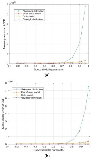
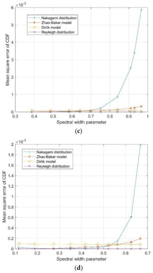
Figure 5.
Comparison of RMS errors in CDF by four frequency-domain methods: (a) Single peak spectrum; (b) bimodal spectrum; (c) multi-peak spectrum; (d) band-limited white noise spectrum.
As can be seen from Figure 5 and Appendix A, the four different life prediction models have the same application conditions and changing rules under different spectrum width parameters, regardless of the form of the simulated spectrum. Since the stress RMS values of these 44 simulated spectrum curves are the same, and the variable is only the spectrum width parameter, the fitting conditions of different life prediction models to the rain flow amplitude can be obtained. The specific analysis results are:
- Histogram of rain flow amplitude: When the root mean square stress is the same, when the spectrum width parameter gradually increases, the stochastic process gradually transits from narrowband to wideband, the distribution of the rain flow amplitude gradually concentrates in the low amplitude area, and the proportion of the high-stress area gradually decreases. That is, the probability of occurrence of low-stress amplitude in a broadband random process is higher than that in a narrow-band random process.
- Rayleigh distribution: When the spectral width parameter ε is small, that is, when approaching a narrow-band random process, the rain flow amplitude distribution is more in line with the Rayleigh distribution, and the fitting effect gradually becomes worse when ε gradually becomes larger. From different cumulative probability density curves, it can be seen that as ε becomes larger, the fitting error in the low-stress region becomes larger, and the probability density value obtained by the Rayleigh distribution will gradually become smaller than the probability density value of the rain flow amplitude. This reduced stress range is also getting larger and larger, which causes a large error when fitting the broadband random process by the Rayleigh distribution. Therefore, it will make the life results too conservative, resulting in the waste of materials.
- Dirlik model: When the spectrum width parameter ε is small, the Dirlik distribution is closer to the Rayleigh distribution. When ε gradually becomes larger, the Dirlik distribution fits the rain flow amplitude histogram better and better, and the shape is closer. The low-stress region can achieve good coincidence, high accuracy, and strong versatility. Especially for broadband random processes with spectral width parameter ε greater than 0.7, the Dirlik model has obvious advantages.
- Zhao–Baker model: The fitting degree of the Zhao–Baker model is similar with the Dirlik model, the difference is that the broadband random process, the Zhao–Baker model will overestimate the part of the low-stress area. Since the area sum of the probability density curve is 1, overestimating the low-stress area will result in underestimating the high-stress area, which will underestimate the fatigue life of the structure and the results will be unsafe.
- Nakagami distribution: Nakagami distribution cannot accurately describe the distribution of rain flow amplitude in the entire stress amplitude range when the spectrum width parameter is small and large. However, in the transition area between the narrow-band random process and the broadband random process, a better fitting effect can be achieved. This is the only distribution model in the four models that can better fit the transition area.
The rain flow amplitude histograms in the figures are obtained by first performing time-frequency conversion on the simulated spectrum to obtain a time history curve, and then performing rain flow counting. Since the simulated spectral curves are the power spectral density curves and do not contain phase information, the time history curves obtained each time are different, and the results of the rain flow count will also be different. However, due to the same statistical characteristics before and after conversion, the trend of the rain flow amplitude histogram obtained by the rain flow counting method with the spectral width parameter value ε is approximately the same. However, it will still cause the above probability density curve and cumulative probability density curve to have certain limitations and errors. At the same time, the analysis of the above graphs shows that the application scope of different frequency-domain methods has certain human factors. The limits of the applicable range cannot be obtained accurately, so the specific life calculation should be combined with the S-N curve of the material and the Miner damage criterion to obtain the accuracy and applicability of different frequency-domain methods through the intuitive numerical relationship.
4.2. Random Fatigue Life Estimation
For the three materials listed in Table 1 and the 44 simulated spectrum curves above, the 10 frequency-domain methods and rain flow counting methods are used to calculate different random fatigue life estimation results TXX.
The life cycle TRF obtained by rain-flow counting method is used as the exact solution, in order to observe the error of each frequency domain method and the exact solution more intuitively, the relative error value RE is taken for analysis. The specific calculation formula is shown in Equation (29):
Performing statistical analysis on the data in the above table and calculating according to Equation (27) obtains the relative error value when calculating random fatigue life by different frequency-domain methods shown in Figure 6, Figure 7 and Figure 8.
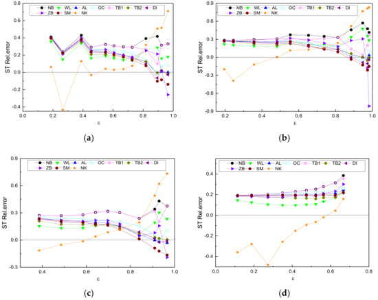
Figure 6.
Comparison of relative errors in estimating fatigue life by frequency-domain method (steel): (a) Single peak spectrum; (b) bmodal spectrum; (c) multi-peak spectrum; (d) band-limited white noise spectrum.
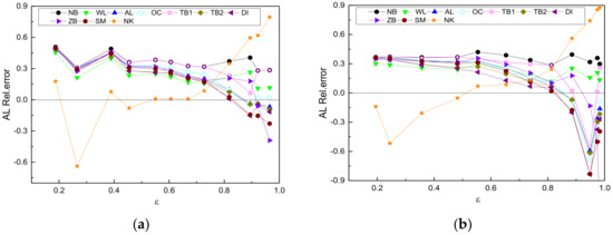
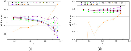
Figure 7.
Comparison of relative errors in estimating fatigue life by frequency-domain method (aluminum alloy): (a) Single peak spectrum; (b) bimodal spectrum; (c) multi-peak spectrum; (d) band-limited white noise spectrum.
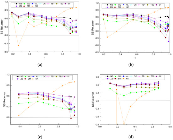
Figure 8.
Comparison of relative errors in estimating fatigue life by frequency-domain method (spring steel): (a) Single peak spectrum; (b) bimodal spectrum; (c) multi-peak spectrum; (d) band-limited white noise spectrum.
Analyzing Figure 6, Figure 7 and Figure 8, we can find that each frequency-domain method has different applicability to different spectrum width parameters and different materials, but it has similar applicability to different spectrum types. Therefore, it can be considered that the accuracy of these 10 frequency-domain methods for calculating random fatigue life is only related to the spectral width parameters and materials, and not to the spectral type. The influence of the material on it is mainly reflected by the influence of the slope k of the S-N curve of the material. When the material is fixed, that is, the m value is fixed, the relative error value of each frequency domain method changes regularly with the change of the spectral width parameter. In addition to the NB method that has been proven to calculate the narrow-band random process, the remaining nine frequency-domain methods are commonly used for the broadband stationary Gaussian random process, so they all show the rule that the errors keep decreasing with the increase of the spectral width parameter, even lower than zero. When the spectrum width parameter is fixed, the applicabilities of each frequency domain method to different slope k values are also different. In general, the increase of k value will cause the calculation error of various frequency-domain methods to increase accordingly, which is very unfavorable for the random fatigue life analysis of materials with a large slope. The specific analysis of the change law of each frequency domain method separately can get the applications of these 10 commonly used frequency domain methods:
- NB method: For the narrow-band stationary Gaussian random process, the distribution of the rain flow amplitude can generally be approximated by the Rayleigh distribution, which has been theoretically confirmed. Through analysis, the NB method is only suitable for narrow-band random processes, but it has poor applicability to the material slope k value.
- WL method: It is a modification of the NB method. When the spectrum width parameter is small, the accuracy of the calculation result is higher than other frequency-domain methods, and the adaptability to the slope k value of the S-N curve is better; when the parameter is large, its accuracy is smaller than those of the frequency domain method applicable to the broadband process. The specific ε application range is roughly 0.1–0.4.
- AL method: Compared with the NB method, the accuracy of the lifetime calculation result of the broadband spectrum is improved, and the applicable range of the spectrum width parameter is roughly 0.75–1.
- TB1 method: Since most of the results of the TB1 method have large errors, only a few data can achieve good results, so the TB1 method is not recommended as a frequency-domain method for calculating random fatigue damage and life in engineering, the scope of application of its spectral width parameter is no longer given here.
- TB2 method: It is suitable for broadband random processes, especially when the spectral width parameter is 0.7–1, the accuracy is high, and it is a commonly used broadband frequency-domain method.
- DI method: The accuracy of the calculation results is similar with TB2, but the accuracy of some regions is slightly lower than TB2. For the ideal broadband random process, the DI method may underestimate the fatigue life results and become dangerous. The applicable range of the spectrum width parameter is roughly 0.7–1, and the DI method is also one of the most widely used methods at present.
- ZB method: For the broadband random process, the accuracy of a small part of the cases is high, but most of the errors are large. The applicable range of the spectrum width parameter is roughly 0.8–0.95.
- OC method: The OC method is also a broadband method, and the applicable range of the spectrum width parameter is roughly 0.85–1.
- SM method: The SM method is also applicable to the broadband process, but for the curve of the ideal broadband random process, when the k value is small, the life will become too high and unsafe. The applicable range of the spectrum width parameter is roughly 0.7–0.9.
- NK method: The NK method has a large error in the calculation results of the ideal narrowband and ideal broadband, but for the transition region of narrowband and broadband, the accuracy of the result is significantly higher than other frequency-domain methods, and it is closer to the exact solution. The applicable range of the spectrum width parameter is approximately 0.45–0.7.
5. Example Analysis
This article will take the canopy of a stadium as the research object. ANSYS, a large-scale general finite element analysis (FEA) software developed by American ANSYS, is used to model and perform random vibration simulation analysis, and the Matlab software is used to perform random fatigue life analysis on the random fatigue response stress power spectral density to verify the results obtained in this paper. The concrete structure and finite element model of the stadium stand canopy are shown in Figure 9.
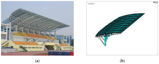
Figure 9.
Stadium stand hood model: (a) Real image; (b) finite element model.
A cantilever steel truss structure is used for the grandstand canopy. The canopy area is 1729 m2 and the amount of steel used is 36.5 kg/m2. The basic members are round steel pipes and the structure is divided into nine steel trusses with a spacing of 7.8 m. Each steel truss consists of two parallel circular arc steel pipes 2.6 m apart to form its upper chord plane, and two circular arc steel pipes joined together form its lower chord, which is connected by a web bar in the middle. Nine steel trusses are connected to the foundation by nine reinforced concrete columns. The steel truss is joined to the column by hinge joints. In order to ensure its geometrical stability, two tension rods extending from the bottom of the column are connected with two upper chord rods, respectively, and then each steel truss is connected into a stable whole by the purlin and the support.
According to the requirements of force and function, five sizes of round steel pipe are used in the structure: upper chordal longitudinal bar Φ168 × 10, lower chordal longitudinal bar 2Φ168 × 10, upper chordal transverse bar, diagonal bar and web bar (excluding support) Φ89 × 4, support web Φ133 × 8, and cable-stayed bar Φ168 × 6. The two lower chords are combined to form a triangular truss system.
The modal analysis of the above finite element model is carried out. First, the dynamic characteristics of the stadium stand canopy model are solved by the modal solution method, and the multi-step natural frequencies and modes are obtained. The first 10 natural frequencies are shown in Table 2.
Table 2.
Calculated natural frequency of structure.
To analyze the stress situation of the structure, this paper mainly considers the effect of wind load. A surface load is applied above the stand shed. To cover the pressure power spectral density of the first 260 natural frequencies, the load frequency range is 0–100 Hz, as shown in Figure 10.
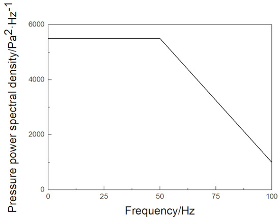
Figure 10.
Pressure load spectrum.
Random vibration spectrum analysis is performed on the stand shed model, and the axial stress and displacement solutions of the stand shed are extracted, as shown in Figure 11.
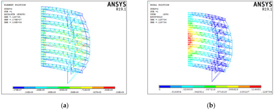
Figure 11.
Finite element results: (a) Axial stress; (b) relative displacement.
The stress power spectral density of the maximum stress point of the response axis is obtained by finite element calculation, as shown in Figure 12.
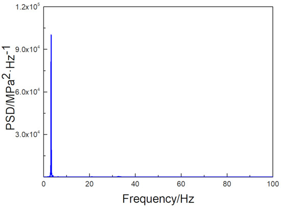
Figure 12.
Response stress power spectral density.
It can be seen from Figure 12 that the first peak of the stress response spectrum occurs at 3.2576 Hz, that is, the second natural frequency of the structure, which corresponds to the mode of the structure. For the stress response, the first peak occupies the main part, and the latter is very small.
The random fatigue life analysis of the structure of the bleacher tent was carried out. First, the axial stress at the maximum stress of the structure is 106.3 MPa. In order to explore the applicability of the change of spectrum width parameters to different frequency domain methods, four sets of power spectra with spectrum width parameters of 0.178, 0.4657, 0.7285, and 0.9611 were generated using Matlab by changing the frequency domain range of the load spectrum. Through different frequency domain methods, the fatigue life of the structure is calculated, and the results are compared using the rain flow counting method as a reference. The estimated results and relative errors are shown in the Table 3:
Table 3.
Random fatigue life estimation results.
Combined with the above analysis results, in general, when the spectral width parameter is 0.1–0.4, the error of the WL method is small; when the spectral width parameter is 0.7–1, the TB2, AL, and DI methods are better than other methods. This is basically consistent with the previous conclusion.
Through the above comparison, we can find that the 10 common frequency-domain methods analyzed in this paper have their own application range of spectral width parameters, but none of the frequency domain methods can be applied to all spectral width parameters or most spectral width parameters. It is only suitable for a small range, and their applicabilities to the slope of the S-N curve of the materials are also uneven. The same frequency domain method will have a large difference in the degree of application of different k values. Through the analysis of the applicable range of the spectral width parameters in this paper, it can provide a reference for selecting an appropriate life prediction model when calculating random fatigue damage or life and reduce errors.
6. Conclusions
The basic knowledge and methods of the fatigue life analysis including the time domain and frequency domain has been presented in this paper. Combining with the simulated spectra and the theory about random vibration and random fatigue strength, the analysis and comparison between different exiting frequency domain methods have been done. The application scope of the spectrum width parameters of 10 commonly used frequency domain methods are emphatically studied, and an engineering example is introduced for verification and analysis. The detailed results are summarized as follows:
- Based on the frequency domain method of random fatigue life estimation theory, the basic principle, advantages and disadvantages of 10 common frequency domain methods are discussed. Then, 44 groups of single-peak spectrum, double-peak spectrum, multi-peak spectrum and band-limited white noise spectrum are simulated to compare the methods in different frequency domains by using steel, aluminum alloy, and spring steel, which are commonly used in engineering.
- Time-domain simulation of 44 groups of spectrum is carried out. The histogram of the rain flow amplitude and cumulative probability density curve of the rain flow amplitude for each curve are obtained by the rain flow counting method and compared with four approximate amplitude probability distribution methods. It can be concluded that four different life prediction models have the same applicability and variation rule under different spectral width parameters, and are independent of the form of simulation spectrum. The results show that the Reyleigh distribution is suitable for fitting narrowband stochastic processes. The Dirlik method has obvious advantages when the spectrum width parameter is larger than 0.7. The Zhao–Baker method fits the broadband stochastic processes well but underestimates the fatigue life of structures. The Nakagami method can better fit the transition region between narrowband and broadband.
- By analyzing and comparing the results of random fatigue life and relative error, it can be found that each frequency domain method has different applicability for different spectral width parameters and different materials, but similar applicability for different spectral shapes. Relative error values of different frequency domain methods increase with increasing slope values of material S-N curves. When analyzing the variation rule of each frequency domain method for a specific material, the applicable ranges of spectrum width parameters of 10 common frequency domain methods are obtained, which can provide reference for choosing the appropriate life prediction model.
- Based on random vibration theory and fatigue life theory, simulation analysis of a stadium grandstand canopy under random vibration conditions was carried out. By changing the spectrum width parameters of the power spectrum, the fatigue life results of the structure are calculated by different frequency domain methods and compared with the rain flow counting method. The results show that when the parameter of spectrum width is 0.1–0.4, the error of the WL method is small, and when the parameter of spectrum width is 0.7–1, the TB2 method and DI method are better than other methods, thus validating the previous conclusions effectively.
Author Contributions
Conceptualization, investigation, and writing: J.X., Y.Z.; investigation: J.L.; review and editing: J.X., Q.H., G.L.; funding acquisition: Q.H. All authors have read and agreed to the published version of the manuscript.
Funding
The authors would like to thank the support from National Natural Science Foundation of China (no. 51525803), the Joint Funds of the National Natural Science Foundation of China (U1939208), and the 111 Project (B20039).
Conflicts of Interest
The authors declare no conflict of interest. The funders had no role in the design of the study; in the collection, analyses, or interpretation of data; in the writing of the manuscript, or in the decision to publish the results.
Appendix A


Figure A1.
Probability density distribution of the amplitude of rain flow (single peak spectrum).


Figure A2.
Rain flow amplitude CDF (single peak spectrum).


Figure A3.
Probability density distribution of the amplitude of rain flow (bimodal spectrum).


Figure A4.
Rain flow amplitude CDF (bimodal spectrum).


Figure A5.
Probability density distribution of rain flow amplitude (multi-peak spectrum).


Figure A6.
Rain flow amplitude CDF (multi-peak spectrum).


Figure A7.
Probability density distribution of rain flow amplitude (band-limited white noise spectrum).


Figure A8.
Rain flow amplitude CDF (band-limited white noise spectrum).
References
- Han, Q.; Li, J.; Xu, J.; Ye, F.; Carpinteri, A.; Lacidogna, G. A new frequency domain method for random fatigue life estimation in a wide-band stationary Gaussian random process. Fatigue Fract Eng. Mater. Struct. 2019, 42, 97–113. [Google Scholar] [CrossRef]
- Wu, Z.; Zhao, Y.; Liang, J.; Fu, M.; Fang, G. A Frequency Domain Approach in Residual Stiffness Estimation of Composite Thin-wall Structures under Random Fatigue Loadings. Int. J. Fatigue 2019. [Google Scholar] [CrossRef]
- He, J. Research on Random Fatigue Strength Analysis Method and Application; Zhejiang University: Hangzhou, China, 2014. [Google Scholar]
- Wei, H.; Carrion, P.; Chen, J.; Imanian, A.; Shamsaei, N.; Iyyer, N.; Liu, Y. Multiaxial high-cycle fatigue life prediction under random spectrum loadings. Int. J. Fatigue 2020, 134, 105462. [Google Scholar] [CrossRef]
- Kang, J.; Liu, H.P.; Fu, D.Y. Fatigue Life and Strength Analysis of a Main Shaft-to-Hub Bolted Connection in a Wind Turbine. Energies 2019, 12, 7. [Google Scholar] [CrossRef]
- Matsuishi, M.; Endo, T. Fatigue of metals subjected to varying stress. Int. J. Jpn. Soc. Precis. Eng. 1968, 68, 37–40. [Google Scholar]
- Lindgren, G.; Rychlik, I. Rain flow cycle distributions for fatigue life prediction under Gaussian load processes. Fatigue Fract. Eng. Mater. Struct. 1987, 10, 251–260. [Google Scholar] [CrossRef]
- Yeter, B.; Garbatov, Y.; Soares, C.G. Fatigue damage assessment of fixed offshore wind turbine tripod support structures. Eng. Struct. 2015, 101, 518–528. [Google Scholar] [CrossRef]
- Park, J.B.; Choung, J.; Kim, K.S. A new fatigue prediction model for marine structures subject to wide band stress process. Ocean Eng. 2014, 76, 144–151. [Google Scholar] [CrossRef]
- Bennebach, M.; Rognon, H.; Bardou, O. Fatigue of Structures in Mechanical Vibratory Environment. From Mission Profiling to Fatigue Life Prediction. Procedia Eng. 2013, 66, 508–521. [Google Scholar] [CrossRef]
- Gao, D.Y.; Yao, W.X.; Wu, T. A damage model based on the critical plane to estimate fatigue life under multi-axial random loading. Int. J. Fatigue 2018, 129, 104729. [Google Scholar] [CrossRef]
- Li, Z.; Ince, A. A new modeling framework for fatigue damage of structural components under complex random spectrum. In Fatigue Design 2019, International Conference on Fatigue Design, 8th ed.; Lefebvre, F., Cetim, P.S., Eds.; Elsevier Science Bv: Amsterdam, The Netherlands, 2019. [Google Scholar]
- Xia, J.; Yang, L.; Liu, Q.; Peng, Q.; Cheng, L.; Li, G. Comparison of fatigue life prediction methods for solder joints under random vibration loading. Microelectron. Reliab. 2019, 95, 58–64. [Google Scholar] [CrossRef]
- Xu, H.L.; Han, Z.X.; Cui, J.Q.; Wei, L.P. Random vibration characteristics and fatigue strength analysis of 7140 passenger car frame. J. Mech. Sci. Technol. 2012, 29, 7–10. [Google Scholar]
- Julian, M.; Denis, B.; Robreto, T. Variance of fatigue damage in stationary random loadings: Comparison between time- and frequency-domain results. Procedia Str. Int. 2019, 24, 398–407. [Google Scholar]
- Dong, B.T.; Shi, R.M.; Zhu, G.R. Estimation of structural fatigue life under random vibration loads. Aircr. Des. 2005, 36–41. [Google Scholar]
- Mrsnik, M.; Slavic, J.; Boltezar, M. Frequency-domain methods for a vibration-fatigue-life estimation—Applicationto real data. Int. J. Fatigue 2013, 47, 8–17. [Google Scholar] [CrossRef]
- Braccesi, C.; Cianetti, F.; Lori, G.; Pioli, D. Fatigue behavior analysis of mechanical components subject to random bimodal stress process: Frequency domain approach. Int. J. Fatigue 2005, 27, 335–345. [Google Scholar] [CrossRef]
- Wang, R.J.; Shang, D.G. Fatigue Life Prediction Based on Natural Frequency Changes For Spot Welds under Random Loading. Int. J. Fatigue 2009, 31, 361–366. [Google Scholar] [CrossRef]
- Wang, M.Z. Research on Life Analysis Method for Structure Vibration Fatigue; College of Aerospace Engineering, Nanjing University of Aeronautics and Astronautics: Nanjing, China, 2009. [Google Scholar]
- Gao, Z.; Moan, T. Frequency-domain fatigue analysis of wide-band stationary Gaussian processes using a trimodal spectral formulation. Int. J. Fatigue 2008, 30, 1944–1955. [Google Scholar] [CrossRef]
- Néron, C.; Padioleau, C.; Blouin, A.; Monchalin, J.P. Robotic laser-ultrasonic inspection of composites. AIP Conf. Proc. 2013. [Google Scholar] [CrossRef]
- Yang, J.; Lee, H.; Lim, H.J.; Kim, N.; Yeo, H.; Sohn, H. Development of a fiber-guided laser ultrasonic system resilient to high temperature and gamma radiation for nuclear power plant pipe monitoring. Meas. Sci. Technol. 2013, 24, 085003. [Google Scholar] [CrossRef]
- Yang, W.J.; Shi, R.M. The distribution law of random vibration stress amplitude. Mech. Des. Res. 2011, 27, 16–20. [Google Scholar]
- Han, C.; Qu, X.; Ding, S.; Ma, Y. A new tri-modal spectral model for evaluating fatigue damage under three or multi-random Gaussian loads. Ocean Eng. 2020, 197, 106708. [Google Scholar] [CrossRef]
- Bendat, J.S.; Piersol, A.G. Measurement and analysis of random data. Technometrics 1966, 10, 869–871. [Google Scholar]
- Wirsching, P.H.; Light, M.C. Fatigue under wide band random stresses. J. Struct. Div. 1980, 106, 1593–1607. [Google Scholar]
- Benasciutti, D.; Tovo, R. Spectral methods for lifetime prediction under wide-band stationary random processes. Int. J. Fatigue 2005, 27, 867–877. [Google Scholar] [CrossRef]
- Dirlik, T. Application of Computers in Fatigue Analysis. Ph.D. Thesis, University of Warwick, Coventry, UK, 1985. [Google Scholar]
- Teixeira, G.M.; Roberts, M.; Silva, J. Random vibration fatigue of welded structures—Applications in the automotive industry. In Fatigue Design 2019, International Conference on Fatigue Design, 8th ed.; Lefebvre, F., Cetim, P.S., Eds.; Elsevier Science Bv: Amsterdam, The Netherlands, 2019. [Google Scholar]
- Zhao, W.W.; Baker, M.J. A new stress-range distribution model for fatigue analysis under wave loading. In Environmental Forces on Offshore Structures and Their Predictions; Springer: Amsterdam, The Netherlands, 1990; pp. 271–291. [Google Scholar]
- Ortiz, K.; Chen, N. Fatigue damage prediction for stationary wideband processes. In Proceedings of the Fifth International Conference on Applications of Statistics and Probability in Soil and Structural Engeenering, Vancouver, BC, Canada, 25–29 May 1987. [Google Scholar]
- Larsen, C.E.; Lutes, L.D. Predicting the Fatigue Life of Offshore Structures by the Single-Moment Spectral Method. Stochastic Structural Dynamics 2; Springer: Berlin/Heidelberg, Germany, 1991; pp. 91–120. [Google Scholar]
- Karagiannidis, G.K.; Sagias, N.C.; Mathiopoulos, P.T. Nakagami: A Novel Stochastic Model for Cascaded Fading Channels. IEEE Trans. Commun. 2007, 55, 1453–1458. [Google Scholar] [CrossRef]
- Wang, M.Z.; Yao, W.X. The amplitude distribution of rain flow in the process of limiting white noise. Chin. J. Aeronaut. 2009, 30, 1007–1011. [Google Scholar]
- Zhang, X.Y. Aircraft structural acoustic fatigue analysis and anti-acoustic fatigue design. Chin. J. Aeronaut. 1992, 13, 197–201. [Google Scholar]
- Fei, Y. Fatigue Life of Structures under Random Vibration Loads. Master’s Thesis, Tianjin University, Tianjin, China, 2017. [Google Scholar]
- Halfpenny, A. A frequency domain approach for fatigue life estimation from finite element analysis. In Key Engineering Materials; Trans Tech Publications Ltd.: Bach, Switzerland, 1999; pp. 401–410. [Google Scholar]
- Calderon-Uriszar-Aldaca, I.; Biezma, M.V.; Matanza, A.; Briz, E.; Bastidas, D.M. Second-order fatigue of intrinsic mean stress under random loadings. Int. J. Fatigue 2020, 130, 13. [Google Scholar] [CrossRef]
© 2020 by the authors. Licensee MDPI, Basel, Switzerland. This article is an open access article distributed under the terms and conditions of the Creative Commons Attribution (CC BY) license (http://creativecommons.org/licenses/by/4.0/).