Notes on a New Structure of Active Noise Control Systems

Abstract

The idea of active noise control is an attenuation of unwanted noise with an additionally generated acoustic wave using the phenomenon of interference. Its technical realization employs advanced control algorithms. Active noise control is an area of intense research and practical engineering applications. In the paper a new structure of adaptive active noise control systems is proposed. Compared with classical control systems used for active noise control, the proposed structure contains in an error signal measurement path an additional discrete-time filter that estimates signal values at the input of this path. These estimates are then used to tune the corresponding adaptive filter. Properties of the proposed adaptive active noise control structure are illustrated by simulation examples in which a feedforward control system equipped with this additional filter is used to attenuate unwanted wide-sense stationary random noises with continuous and mixed spectra.

1. Introduction

Active noise control is a very interesting technique used presently by researchers and engineers in different areas of their activity. This technique is applied for attenuation of unwanted waves as well as for the generation of random fields with desired spectral properties [1,2,3]. It has a well-established theory that allows one to design hardware and software for adaptive and non-adaptive, single and multi-channel active noise control systems [4,5,6,7,8]. Active noise control techniques utilize a number of control system structures and control algorithms to attenuate unwanted noise. A feedforward control system structure is applied if measurements of a reference signal giving an additional knowledge about the noise to be attenuated can be obtained. Feedback control system structures are utilized when there are problems with the reference signal acquisition. This implies that values of the reference signal have to be estimated using ideas of the internal model control [6,9]. Commonly, adaptive control algorithms are applied for the tuning of active noise controllers for two reasons: Initially, to calculate controller coefficients, and next, to update these coefficients to time-varying properties of the noise and the controlled electro-acoustic plant. Adaptation may be performed either in time or in frequency domain basing on the error signal, picked up by the error microphone and then processed by an electronic hardware being the measurement path (an amplifier, antialiasing filter, and A/D converter). Such a processed error signal is used to calculate the coefficients of the active noise controller by minimizing at consecutive discrete-time instants an objective function, that being the corresponding mean square value. For this minimization, an algorithm from a family of least mean square (LMS) algorithms may be applied [10].

It follows from the control theory that each adaptive active noise control system is a nonlinear and time-varying dynamic system, in which the signal at the error microphone and error signal seen by the adaptation algorithm are connected by a nonlinear dynamic relation [11,12]. Consequently, an adaptation process conducted using the signal obtained at the output of the measurement path may not lead to the greatest possible noise attenuation at the error microphone and the greatest rate of convergence of an adaptation algorithm. To get closer to the optimal solution a modification of an adaptation process is proposed. Its idea is the following: In the adaptation process the input signal of the error signal measurement path is used instead of the corresponding signal output. This input signal is not technically measurable but its values can be estimated using signal processing algorithms. The active noise control algorithm using these signal estimates is considered in the paper. Its origination may be found in a control system structure called the filtered-reference filtered-error LMS (FeFxLMS) algorithm. In this algorithm, an additional discrete-time filter is placed in the error signal measurement path following the A/D converter. This filter may be used for residual error shaping in active noise control [13,14,15,16,17] or to increase the rate of convergence of the adaptation process [18,19,20,21,22]. In the paper, a new functionality, not addressed earlier is assigned to this filter. It returns estimates of a signal at the input of the error signal measurement path that are next used in the adaptation process. It is shown in the paper that these estimates influence the behavior of active noise control systems increasing obtained noise attenuation at the error microphone and rate of convergence of active noise control algorithms.

The paper is organized as follows: (1) The problem of the lack of optimality of classical active noise control system designs is stated; (2) a new active noise control system structure that uses estimates of signal at the input of error signal measurement path in adaptation process is proposed; and (3) properties of the proposed new active noise control system structure are illustrated by simulation case studies of attenuation of wide-sense stationary Gaussian random noises with continuous and mixed spectra in active noise control structures employing models of electro-acoustical plants with different dynamical properties.

2. Problem Statement

The ideas presented in the paper are discussed below using as an example a classical feedforward active noise control system structure called FxLMS (filtered-reference least mean square) algorithm [4,5,7,8,23]. A block diagram of this control system structure is shown in Figure 1. Blocks appearing in the figure are defined below on an example of an active noise control system creating local zones of quiet in an enclosure. The terminology used is also explained in Figure 2 that shows a laboratory configuration applied as a model for simulations included in the paper.

An unwanted wide-sense stationary random noise propagates in an acoustic space of the enclosure from a primary source to an error microphone around which a local zone of quiet is created. In the error microphone, the noise to be attenuated meets a signal generated by the control loudspeaker driven by a control signal $u\left(i\right)$ (where $i=0,1,\dots$ denotes consecutive discrete-time instants). These two signals interfere. The result of interference is picked up by the error microphone and is next processed by an electronic path consisting of an amplifier, analogue antialiasing filter, and A/D converter (the hardware forming an error signal measurement path). At the output of this path, numbers that are a discrete-time error signal $e\left(i\right)$ are obtained. The acoustic space between the primary noise source and error microphone as well as elements of the error signal measurement path together with dynamics of a noise generation system form the disturbance path. The noise generation system is a device transforming the mathematical definition of the noise to be attenuated into a realization of a random process that is further processed into the corresponding acoustic wave. The disturbance path is introduced for the precise definition of the models used in simulations.

The control signal $u\left(i\right)$ is an output of a time-varying FIR (finite impulse response) filter $W\left(z^{-1}\right)$ ($z^{-1}$ denotes one-step delay operator) that is adaptively tuned at each discrete-time instant i. It reaches the error microphone after processing by the D/A converter equipped with a zero-order hold filter, analogue forming filter, amplifier, control loudspeaker, and acoustic space. These elements together with the components of the error signal measurement path like the error microphone, amplifier, analogue antialiasing filter, and A/D converter form the secondary path. An input signal of the filter $W\left(z^{-1}\right)$ is a signal that is returned by a reference microphone placed in a vicinity of the primary source of noise. Dynamics of this microphone together with dynamics of the electronic elements converting the noise at the primary source (its mathematical definition) into numbers forming a discrete-time reference signal $x\left(i\right)$ is called a reference signal measurement path. This path similarly like the disturbance path was introduced for a simulation purpose only.

The discrete-time signal $x\left(i\right)$ processed additionally by a model of the secondary path together with the discrete-time signal $e\left(i\right)$ is used by the LMS algorithm to tune the filter $W\left(z^{-1}\right)$ so that mean square values $\mathcal{E}\left\{e^2\left(i\right)\right\}$ ($\mathcal{E}\left\{·\right\}$ denotes the expectation operator) are minimized for each discrete-time instant i. It must be emphasized that the use of the signal $e\left(i\right)$ in the adaptation process is not an optimal solution from the point of view of the active noise control system users. It would be optimal if instead of using the mentioned signal $e\left(i\right)$ (the output of the error signal measurement path), the corresponding input signal $e_0\left(i\right)$ of this path (see Figure 3) is used in the adaptation process. It means that to tune the filter $W\left(z^{-1}\right)$ the values of $\mathcal{E}\left\{e_0^2\left(i\right)\right\}$ should be minimized by the LMS-based algorithm at each discrete-time instant i. Consequently, the discrete-time signals $e\left(i\right)$ or $e_0\left(i\right)$ are connected by a nonlinear and time-varying dynamic relation during active adaptation process [11,12]. It follows from this nonlinear and time-varying nature of the adaptive system that noise reduction obtained with the adaptive active noise control system tuned with the discrete-time signals $e\left(i\right)$ or $e_0\left(i\right)$ may give different results. It implies also that obtaining minimum of $\mathcal{E}\left\{e^2\left(i\right)\right\}$ does not guarantee obtaining a minimum of $\mathcal{E}\left\{e_0^2\left(i\right)\right\}$ for the consecutive discrete-time instants and vice versa.

In Figure 3 the error signal measurement path is presented as excluded from the disturbance and secondary paths. As a result the secondary path is shown as a serial connection of the secondary path control signal part and error signal measurement path. Consequently, the disturbance path consists of the acoustical disturbance path and error signal measurement path. The output of the acoustical disturbance path is the noise to be attenuated. It is denoted by $d\left(i\right)$. It should be emphasized that it is not the discrete-time signal at the output of the disturbance path in Figure 1 that models an approximate influence of the noise to be attenuated on the error signal seen by the adaptation algorithm.

3. A New Structure of Active Noise Control Systems

Values of the discrete-time signal $e_0\left(i\right)$ are not technically measurable but they can be estimated with a signal processing algorithm. The technical realization of this idea results in a new structure of an active noise control system presented in Figure 4. To estimate values of the discrete-time signal $e_0\left(i\right)$ a discrete-time filter FIR with a transfer function $F_{est}\left(z^{-1}\right)$ is included into the secondary path (and into the disturbance path as well) at the output of error signal measurement path. This filter should also be taken into account as a part of the secondary path model. The resulting active noise control system structure is known in the literature as a FeFxLMS control system structure [13,14,15,16,17,18,19,20,21,22]. The literature FeFxLMS is used in another way: To shape properties of the error signal seen by the adaptation algorithm (not perceived by the active noise control system users) as well as to accelerate the rate of convergence of the adaptation algorithm based on the discrete-time signal $e\left(i\right)$. A special case, filtered-error LMS (FeLMS) also uses a filter placed in the error signal measurement path to compensate for the secondary path effects [4,7,24,25,26,27]. However, in the literature the existence of the error signal measurement path is not treated in a correct way from the point of view of control theory. The error signal measurement path is included into the primary and secondary paths. It is an optimal solution only for an unrealistic case of the error signal $e\left(i\right)$ equal to 0. In this case the error signal $e_0\left(i\right)$ at the error microphone is also equal to 0.

In the paper the coefficients of the filter $F_{est}\left(z^{-1}\right)$ are calculated offline, before the activation of the active noise control system, using a routine for the equalization of communication transmission channels [28,29,30]. It means that the following objective function:

$$\mathcal{E}\left\{{\left({\widehat{e}}_0\left(i\right)-e_0(i-\Delta )\right)}^2\right\}$$

(1)

is minimized with the LMS, LS (least squares), or the RLS (recursive least squares) algorithm and an artificially offline generated discrete-time signal $e_0\left(i\right)$. Realizations of persistently exciting signals of a proper order should be used as $e_0\left(i\right)$ [31]. In the objective function (1) ${\widehat{e}}_0\left(i\right)$ is the output of a discrete-time filter $F_{est}\left(z^{-1}\right)$ excited by the output $e\left(i\right)$ of the error signal measurement path and $\Delta$ is a discrete-time delay being the parameter of equalization algorithm. It is assumed that the dynamical model of the error signal measurement path is known before the equalization is performed and may be identified offline in any way before the start of the active noise control system [32]. Values of $e\left(i\right)$ necessary for equalization are calculated using the known model of the error signal measurement path and artificially generated values of discrete-time signal $e_0\left(i\right)$ used as the excitation of the model of the error signal measurement path. It is worth noticing that the identified linear dynamical model of the error signal measurement path may contain unstable zeros that influence the quality of estimates ${\widehat{e}}_0\left(i\right)$ obtained. An offline calculation of the filter $F_{est}\left(z^{-1}\right)$ coefficients may be considered as an inverse modeling of the error signal measurement path in the minimum variance sense and this filter is called in the paper an equalization filter. The use of identification techniques for inverse modeling overcomes problems associated with inverting dynamic systems with unstable zeros.

The filter $F_{est}\left(z^{-1}\right)$ may be incorporated into the error signal measurement path as an additional hardware or into the adaptive control algorithm implemented in a signal processor. Included into the active noise control algorithm the filter $F_{est}\left(z^{-1}\right)$ increases the computational burden necessary to calculate control signal values by maximally two additional FIR filtrations more than for the FxLMS algorithm.

After the successful equalization of the error signal measurement path by the discrete-time filter $F_{est}\left(z^{-1}\right)$ and with the assumption that the noise to be attenuated is a wide-sense stationary random process the mean square values $\mathcal{E}\left\{e_0^2\left(i\right)\right\}$ and $\mathcal{E}\left\{{\widehat{e}}_0^2\left(i\right)\right\}$ should be near equal. It means that values ${\widehat{e}}_0\left(i\right)$ seen by the adaptation algorithm are a good estimate of values $e_0\left(i\right)$ picked up by the error microphone and perceived by the active noise control system users. It also implies that noise reduction perceived by the active noise control system users is approximately equal to the reduction of the error signal estimate seen by the adaptation algorithm.

4. Simulation Case Studies

The simulation case studies described below are arbitrarily designed to show some basic properties of the proposed new FeFxLMS active noise control structure. All simulations are done in Matlab according to the block diagrams are shown in Figure 3 and Figure 4.

Models of the reference signal measurement path, disturbance path, acoustical disturbance path, secondary path, secondary path control signal part, and error signal measurement path used in the first two simulation case studies are simplified to focus on properties of the presented new FeFxLMS control system structure. In the third simulation case study the corresponding models identified in the laboratory room are used. All models used in simulations are FIR filters with 100 coefficients.

It is assumed in the presented below simulation case studies that: The active noise control systems operate with the constant sampling frequency equal to 500 Hz; an acoustic feedback between the control loudspeaker and the reference microphone is perfectly canceled; simulations started from the time instant 0 and adaptation is activated at the iteration number 1000; the number of FIR filter $W\left(z^{-1}\right)$ coefficients is equal to 50 and are tuned online using the LMS algorithm from initial values equal to 0; $\mu$ parameter (convergence coefficient) is chosen individually for each simulation experiment, the same for both control system structures; the number of FIR filter $F_{est}\left(z^{-1}\right)$ coefficients is 100 and the value of parameter $\Delta$ is equal to 50; and the same realizations of the noise to be attenuated are used to simulate the classical FxLMS and new FeFxLMS control system structures. Additionally, the same model is used to simulate the secondary path and as a model of secondary path. The dynamics of the error microphone present in the error signal measurement path as well as dynamics of the amplifier are omitted in the simulations: It is assumed that dynamics of the error signal measurement path is represented only by dynamics of the antialiasing filter. Such a simplification has no influence on general conclusions drawn. To run the new FeFxLMS control system structure with an estimation of signal values at the error microphone the coefficients of the filter $F_{est}\left(z^{-1}\right)$ are calculated with equalization methods.

With given (offline identified) models of the disturbance, secondary and error signal measurement paths corresponding to the acoustical disturbance path and secondary path control signal part are calculated using model identification algorithms as well as the model of the error signal measurement path. All FIR models obtained in this way are truncated to 100 coefficients.

Power spectral densities of the discrete-time signals presented in the paper are estimated by the averaging of periodograms calculated for non-overlapping data segments [33] taken from a single realization of the corresponding signal. They are obtained using 1500 consecutive data segments consisting each of 1024 signal samples. The calculation of each estimate starts after all transients implied by initial conditions and initial adaptation have decayed.

The time plots of mean square values of signals presented in the paper are obtained by the averaging of curves obtained for 100 or 50 realizations of the noise to be attenuated. Single estimates of the mean square values of the corresponding signals at consecutive discrete-time instants i are obtained as a result of the filtration of squared values of these signals through the first-order discrete-time filter with a gain equal to 1 and an autoregressive parameter equal to 0.999 or 0.99 [34].

Noise reduction obtained in the simulation case studies is estimated as a ratio of the mean square values of the discrete-time signals at the error microphone without and the active noise control system, expressed in dB. Its calculation is performed for the last 10% of the signals after all transients implied by initial conditions have decayed.

4.1. Case Study 1

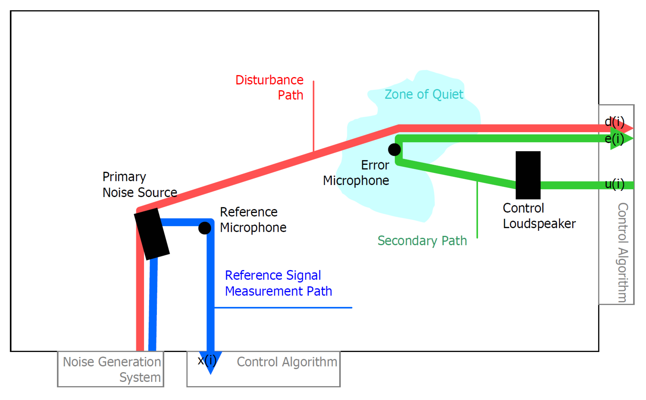
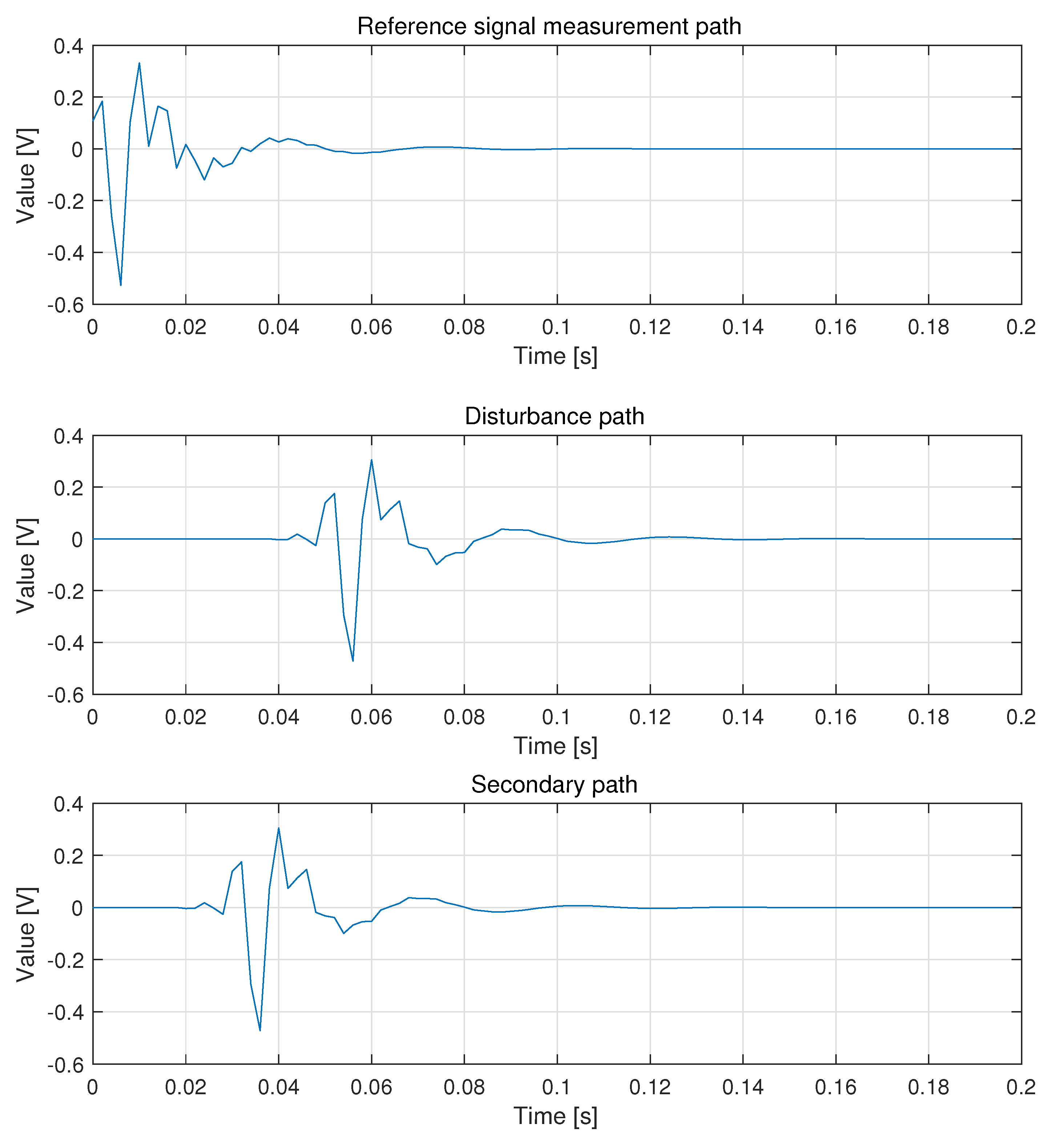
The first simulation case study concerns a problem of the active control of a noise to create a three-dimensional zone of quiet in a space without reverberations. Impulse responses of the secondary, disturbance, and reference signal measurement paths used in simulations are presented in Figure 5. They are applied as coefficients of the corresponding FIR filters. In the presented simulation case study the total delay introduced by the error signal measurement path, controller, and secondary path (22 ms) is less than the delay introduced by the disturbance path (40 ms).

To present an influence of the error signal measurement path on the discrete-time signal $e_0\left(i\right)$ from secondary and disturbance paths the discrete-time model of an antialiasing analogue filter has been extracted to obtain models of the acoustical disturbance and secondary path control signal paths. This filter is a low-pass filter with a pass-band limited by 150 Hz and a stop-band starting from 200 Hz. Its sampled impulse response is shown in Figure 6. It is used in simulations as a FIR filter with 100 coefficients. In Figure 6 the corresponding impulse response of the equalization filter $F_{est}\left(z^{-1}\right)$ is also presented.

In simulations presented in the first simulation case study, the coefficients of the FIR filter $W\left(z^{-1}\right)$ are tuned online by the LMS algorithm with the parameter $\mu =0.1$. The noise to be attenuated is a low-correlated wide-sense stationary Gaussian random process with continuous spectrum and a power spectral density at the error microphone shown in Figure 7 and Figure 8 with red lines.

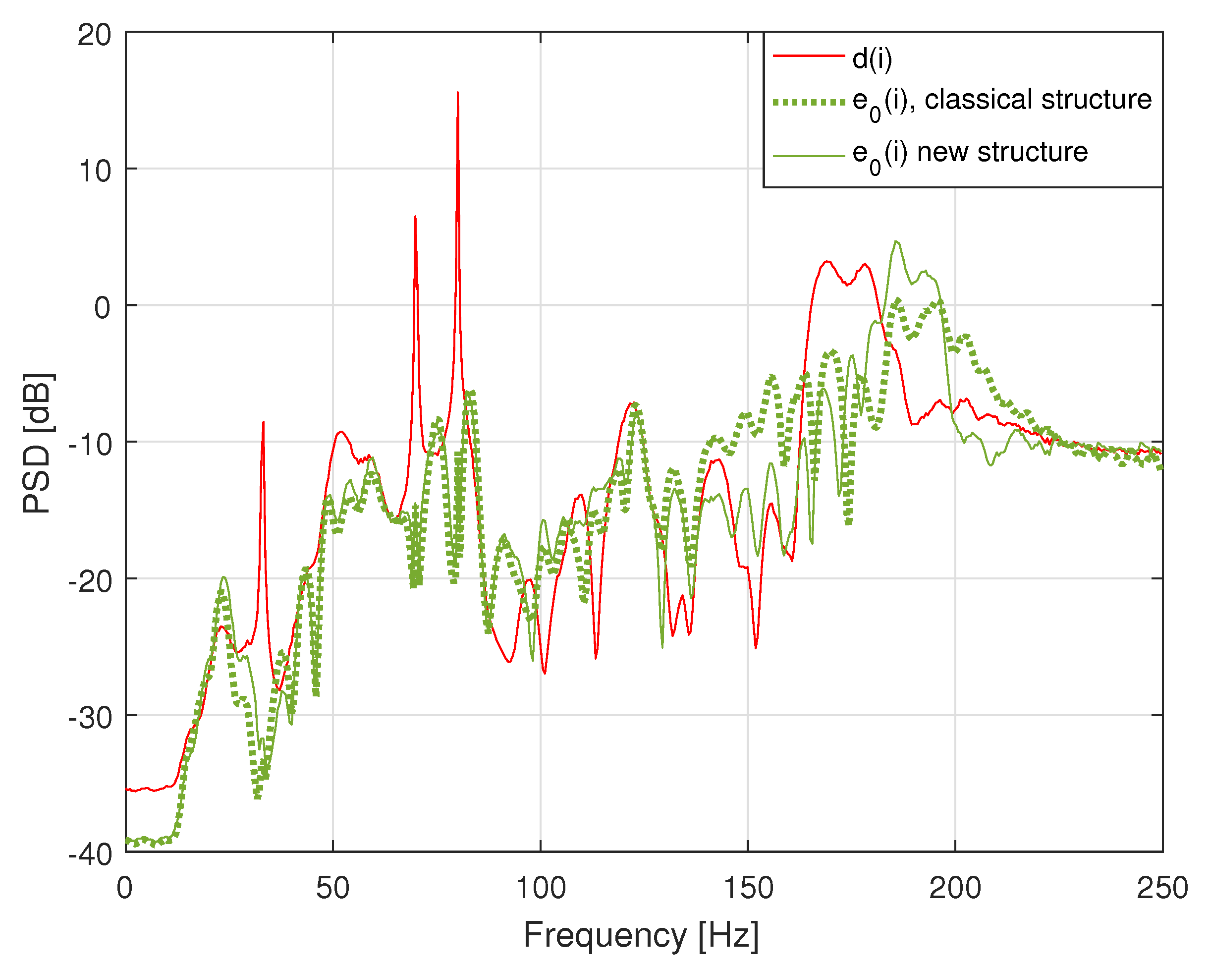
In Figure 7a comparison of the power spectral densities of the discrete-time signals $e\left(i\right)$ and $e_0\left(i\right)$ in the classical FxLMS control system structure as well as a similar comparison of the power spectral densities of the discrete-time signals $e\left(i\right)$, $e_0\left(i\right)$, and ${\widehat{e}}_0\left(i\right)$ in the new FeFxLMS control system structure is presented. It exposes that the difference between the power spectral densities of the discrete-time signals $e\left(i\right)$ and $e_0\left(i\right)$ in the classical FxLMS control system structure is greater that the corresponding difference between the power spectral densities of the discrete-time signals $e_0\left(i\right)$ and ${\widehat{e}}_0\left(i\right)$ in the new FeFxLMS control system structure. 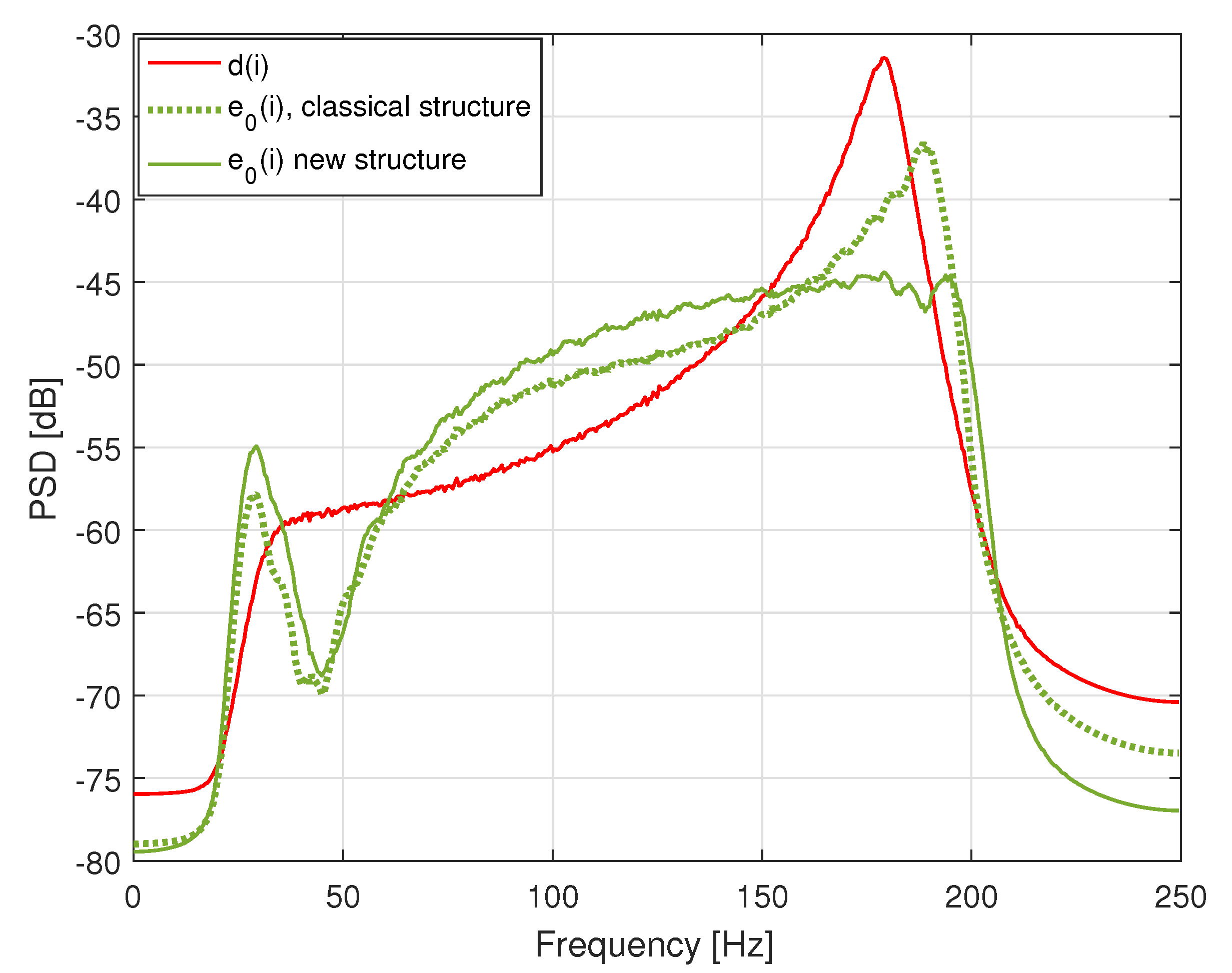It implies also that a calculation of noise reduction obtained based on the signal seen by the adaptation algorithms is more biased in the classical FxLMS control system structure than in the new structure; an estimate of the noise reduction obtained based on the discrete-time signal ${\widehat{e}}_0\left(i\right)$ in the new FeFxLMS control system structure is closer to the noise reduction obtained at the error microphone and consequently, to what the active noise control system user perceives. The comparison of the power spectral densities of the discrete-time signals $e_0(i$) for the classical FxLMS and new FeFxLMS control system structure presented in Figure 8 shows that the new FeFxLMS control system structure gave a significant improvement in the band 150 to 200 Hz due to the influence of the amplitude frequency response of the filter $F_{est}\left(z^{-1}\right)$.

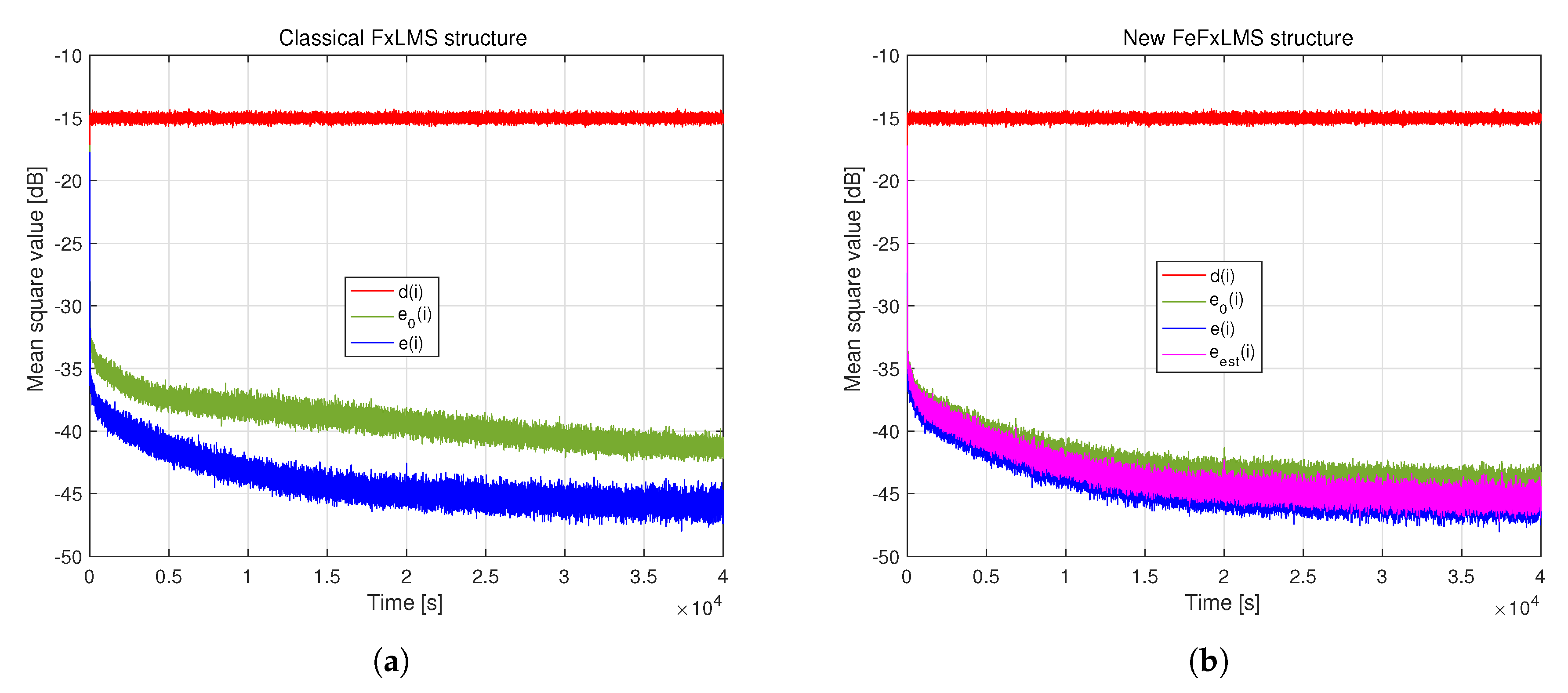
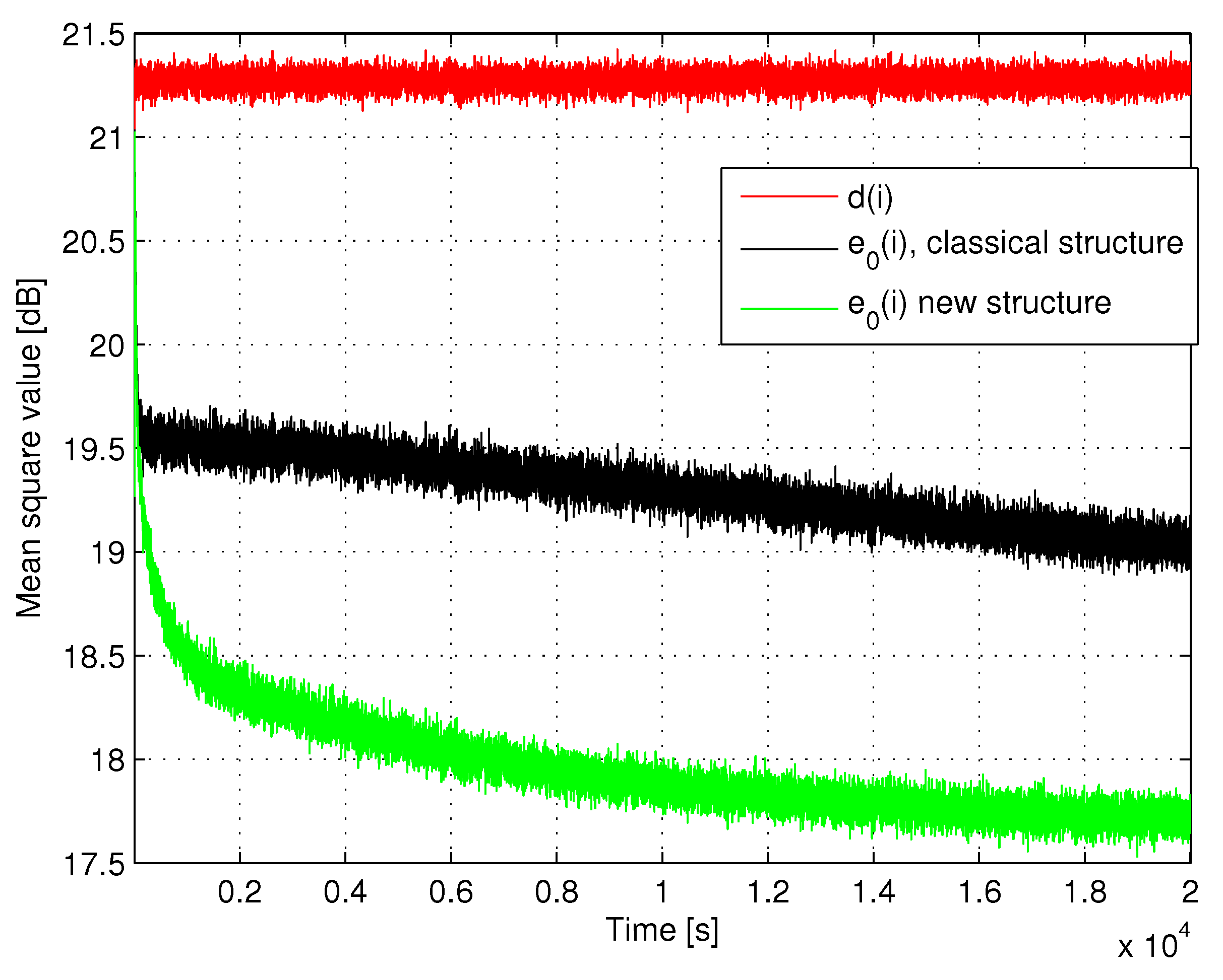
To compare the rate of convergence of the control algorithms in the two discussed structures, the time plots of the discrete-time signals $e\left(i\right)$ and $e_0\left(i\right)$ in the classical FxLMS active noise control system structure as well as the time plots of the discrete-time signals $e\left(i\right)$, $e_0\left(i\right)$, and ${\widehat{e}}_0\left(i\right)$ in the new FeFxLMS active noise control system structure are presented in Figure 9. These are the averaged curves obtained for 100 realizations of noise to be attenuated with the autoregressive parameter equal to 0.999. For the considered noise to be attenuated, the discrete-time error signal $e_0\left(i\right)$ in the new FeFxLMS control system structure converged significantly faster than the signal $e_0\left(i\right)$ in the classical FxLMS control system structure. The plots also show that application of the new FeFxLMS active noise control system structure also gave an improvement in the full frequency band of system operation during initial adaptation. The values of the resulting noise reduction obtained in the classical FxLMS and new FeFxLMS control system structures are reported in

Table 1. Noise reduction: Continuous spectrum low-correlated case.

Signal	Classical FxLMS Structure	New FeFxLMS Structure
$e_0\left(i\right)$	$26.2$ dB	$29.0$ dB
$e\left(i\right)$	$30.9$ dB	$30.9$ dB
${\widehat{e}}_0\left(i\right)$	$----$	$30.4$ dB

. It is worth emphasizing that with the new FeFxLMS control system structure, a greater noise reduction (approximately 10%) in error microphone (signal $e_0\left(i\right)$) was observed. No perfect equality of noise reduction obtained seen by the error microphone and adaptive control algorithm was obtained due to a non-minimum phase feature of the error signal measurement path and the nonlinear feedback introduced by the adaptation algorithm [11,12].

4.2. Case Study 2

In the second simulation case study, dynamic properties of the disturbance and secondary paths are changed to represent a dynamic system in which the prediction of the noise to be attenuated is more difficult than in the previous simulation case study. The total time delay in the error signal measurement path, controller, and secondary path (14 ms) is longer than that the time delay in the disturbance path (6 ms). The corresponding impulse responses are presented in Figure 10.

The above change implies that the low correlated noise used in the previous simulation case study could not be effectively attenuated. To obtain a visible noise reduction, the power spectral density of noise to be attenuated was also changed to a power spectral density defining a highly correlated wide-sense stationary Gaussian random noise. Its power spectral density is presented in Figure 11 and Figure 12 with red lines. This noise was attenuated in the classical FxLMS and new FeFxLMS control system structures. Parameters of the adaptive control algorithms were the same as for the previous simulation example except of the parameter $\mu$ that was equal to 0.03.

In Figure 11, the estimated power spectral densities of the discrete-time signals $e\left(i\right)$ and $e_0\left(i\right)$ in the classical FxLMS control system structure and corresponding estimates for the new FeFxLMS control system structure calculated using the discrete-time signals $e\left(i\right)$, $e_0\left(i\right)$, and ${\widehat{e}}_0\left(i\right)$ are presented. Power spectral densities of the discrete-time signals $e_0\left(i\right)$ estimated in the classical FxLMS and new FeFxLMS control system structures are compared in Figure 12.

Noise reduction obtained with the classical FxLMS and new FeFxLMS control system structures is presented in

Table 2. Noise reduction—continuous spectrum highly correlated case.

Signal	Classical FxLMS Structure	New FeFxLMS Structure
$e_0\left(i\right)$	$3.3$ dB	$5.4$ dB
$e\left(i\right)$	$8.4$ dB	$7.4$ dB
${\widehat{e}}_0\left(i\right)$	$----$	$5.4$ dB

. Similarly, as in the previous simulation case study, the new FeFxLMS control system structure gave a greater (approximately 50%) noise reduction in the error microphone (signal $e_0\left(i\right)$). It was also observed that similarly to the previous case study, the discrete-time signal $e_0\left(i\right)$ exposed a greater rate of convergence in the new FeFxLMS control system structure than in the classical FxLMS control system structure.

In the next step, the rate of convergence of the discrete-time signal $e_0\left(i\right)$ is compared in the classical FxLMS and new FeFxLMS control system structures in simulations run to attenuate another noise. It is a wide-sense stationary random process with a mixed spectrum defined at the primary noise source, as a sum of two random sines and a discrete-time Gaussian white noise with a given variance. The random sine components frequencies were equal to 50 and 120 Hz, the amplitudes were equal to 1, and the phase shifts were random, equally distributed in the range $[0,2\pi )$. It should be noted that the Gaussian white noise after processing by dynamics of the reference signal measurement path and acoustical disturbance path was no longer white. Its power spectral density at the error microphone looked similar to the power spectral density of the noise used in the first simulation case study.

For a chosen variance of Gaussian white noise, 1000 realizations of 50,000 samples of the mixed spectrum random noise were generated and simulations were conducted. Parameter $\mu$ was equal to 0.003. At each iteration, the corresponding mean square values of the discrete-time signal at the error microphone were estimated with the autoregressive parameter equal to 0.99, averaged over 1000 realizations, and expressed in dB. Next, differences between pairs of mean square value estimates in the classical FxLMS and new FeFxLMS control system structures are presented in Figure 13 for the variance of Gaussian white noise equal to 0, 0.0001, 0.001, 0.01, 1, and 2.

The resulting difference was greater than zero for each Gaussian noise variance chosen. Consequently the noise reduction obtained in the new FeFxLMS control system structure was greater than in the classical FxLMS control system structure. Additionally, the time plots of the differences between expressed in dB estimates of the mean square value of the signals at the error microphone show that adaptation was faster in the new FeFxLMS than in the classical FxLMS control system structure during the whole simulation time and in general significantly faster during the initial adaptation period.

4.3. Case Study 3

The models of the reference signal measurement, disturbance, and secondary paths used in the previous two simulation case studies had similar amplitude frequency responses but different phase characteristics implied by the corresponding time delays in the signal processing paths. To verify the research results in the third simulation case study, the models of the reference signal measurement path, acoustical disturbance path, secondary path control signal part, and error signal measurement path identified in a laboratory room were applied. These models (impulse responses) in the form of the corresponding FIR filters were identified offline with the LS method using multisine excitations [35]. For the purpose of simulations, they were cut to the first 100 elements.

The active noise control system was used to create a local zone of quiet in the 70 m${}^3$ reverberant room in the laboratory configuration shown in Figure 2 and Figure 14. The room was disturbed by noises generated from a primary noise source being a loudspeaker driven from a computer by a forming filter and amplifier. Near the primary noises source (0.4 m), a reference microphone was placed. The error microphone was placed 1.8 m from the primary noise source. The control loudspeaker was placed 2.3 m from the primary noise source, and 1 m from the error microphone. It was driven from the dSPACE DS1104 R&D Controller Board by a forming filter and amplifier The signal picked up by the error microphone was further amplified and processed by an antialiasing Butterworth 4th order filter with a cut off frequency equal to 120 Hz and fed to the control algorithm implemented in the controller board. The loudspeakers were Arton Audio Klasyk 70L Subwoofers with Alcone Acoustic AC10HE cones and as the reference and error microphones Beyerdynamic MM1 measurement microphones were employed.

The chosen laboratory configuration implies that the total time delay introduced by the error signal measurement path, controller, and secondary path (22 ms) was longer than the time delay introduced by the disturbance path model (14 ms). Dynamical properties of the laboratory plant are summarized in Figure 15 in which amplitude frequency responses of the reference signal measurement path, acoustical disturbance path, secondary path control signal part, and error signal measurement path (represented by the atialiasing filter) are shown.

In the first step, the rate of convergence of the discrete-time signal $e_0\left(i\right)$ is compared in the discussed active noise control system structures in simulations run to attenuate a noise with a mixed spectrum. The mixed spectrum noise is a sum of three random sines and a discrete-time Gaussian white noise with a given variance. The sine components frequencies were equal to 33, 70, and 80 Hz, amplitudes were equal to 1 and phase shifts that were random, equally distributed in the range $[0,2\pi )$. Such a random process is the input of the reference signal measurement and acoustical disturbance paths. For a given variance of the Gaussian white noise, 1000 realizations of this random process were generated, each realization of 50,000 samples and the classical FxLMS and new FeFxLMS control systems were simulated. Parameter $\mu$ was equal to $5\times {10}^{-6}$. Each realization of the discrete-time signal $e_0\left(i\right)$ was processed in the same way as in the previous simulation case study. Differences between them are expressed in dB estimates of the mean square values of the discrete-time signals $e_0\left(i\right)$ in classical FxLMS and new FeFxLMS control system structures are presented in Figure 16 for the variance of Gaussian white noise equal to 0, 0.0001, 0.001, 0.01, 1, and 2. These differences were greater than 0 and thus show that adaptation was faster in the new FeFxLMS control system structure than in the corresponding classical FxLMS control system structure in the simulation time window of 50,000 samples.

In the next step the length of simulation time window was changed to ${10}^7$ samples and the noise reduction obtained after the convergence of adaptation algorithm was estimated. The obtained results of the mixed spectrum noise reduction are summarized in

Table 3. Noise reduction—mixed spectrum case in a laboratory model.

Variance of White Noise	Classical FxLMS Structure	New FeFxLMS Structure
0	$179.8$ dB	$179.9$ dB
$1\times {10}^{-4}$	$36.9$ dB	$37.4$ dB
$1\times {10}^{-3}$	$27.0$ dB	$28.2$ dB
$1\times {10}^{-2}$	$17.5$ dB	$18.9$ dB
$1\times {10}^{-1}$	$9.2$ dB	$9.5$ dB
1	$3.0$ dB	$1.6$ dB
2	$2.0$ dB	$-1.5$ dB

.

It is important to note that the obtained noise attenuation in the new FeFxLMS control system structure and classical FxLMS control system structure are the same, provided that the error signal $e\left(i\right)$ is equal to 0 and consequently the error signal $e_0\left(i\right)$ at the error microphone is equal to 0 as well. As it was mentioned, it was the only case in which the classical FxLMS control system structure could give an optimal result. For most of the attenuated noises, the results obtained in the new FeFxLMS control system structure were better than what was obtained in the classical FxLMS control system structure, besides the cases with Gaussian white noise variances equaled to 1 and 2. Consequently, the power spectral densities estimated for the variance equal to 1 for a single realization of the discrete-time signals at the error microphone are presented in Figure 17. The power spectral density of the mixed spectrum noise at the error microphone was plotted with a red line and the power spectral densities or the discrete-time error signals $e_0\left(i\right)$ in the classical FxLMS and new FeFxLMS control system structure are plotted with green lines. The noise components placed around the frequency 175 Hz were amplified by the new FeFxLMS control system structure more than by the classical FxLMS control system structure, which indicated that the parameter $\mu$ of was too large. The parameter $\mu$ for the variance of Gaussian white noise equal to 2 was too large as well.

According to the above conclusion, the simulations were repeated with the parameter $\mu$ decreased 100 times to the value $5\times {10}^{-8}$ for Gaussian white noise variances equal to 1 and 2. In Figure 18, the estimated mean square values of the discrete-time signals $e_0\left(i\right)$ for the Gaussian white noise variance equal to 1 are compared; the presented curves averaged for 50 realizations of $d\left(i\right)$. It follows that adaptation in the new FeFxLMS control system structure for the lower $\mu$ value was significantly faster than in the classical FxLMS control system structure. It results in a greater noise reduction (3.40 dB) obtained with the new FeFxLMS algorithm after convergence of the adaptation process. The corresponding noise attenuation obtained with the classical FxLMS algorithm was reduced to 2.2 dB in comparison with the result from Table 3. A similar improvement was observed in the results of the simulation experiments repeated for the Gaussian white noise variance equal to 2 and parameter $\mu$ equal to $5\times {10}^{-8}$. The noise reduction values obtained were 1.79 dB for the classical FxLMS control system structure and 2.78 dB for the new FeFxLMS control system structure.

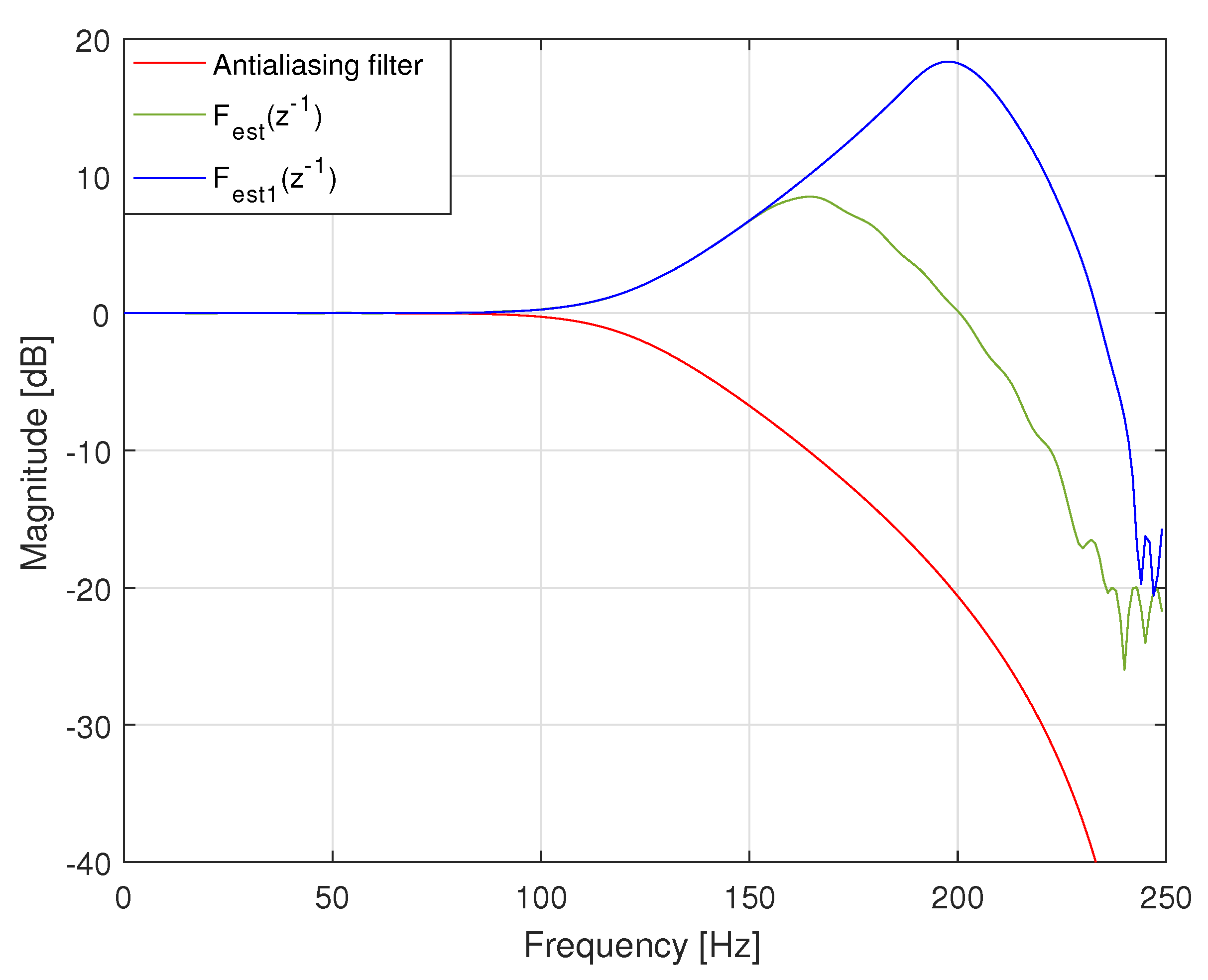
In the last simulation experiments, the influence of the equalization filter precision was addressed. A new filter $F_{est1}\left(z^{-1}\right)$ was applied to estimate values of signal at the error microphone. It was designed to estimate signal values at the error microphone precisely for a wider band of frequencies than it was possible with the filter $F_{est}\left(z^{-1}\right)$. Amplitude frequency responses of the two compared filters are shown in Figure 19. The corresponding simulation results are summarized in Figure 20 and Figure 21.

The noise to be attenuated is the continuous spectrum wide-sense stationary Gaussian random noise defined by the power spectral density plotted with a red line in Figure 21. Simulation experiments were repeated for its 50 realizations of ${10}^6$ samples. The parameter $\mu$ was equal to $5\times {10}^{-7}$. In Figure 20, the estimated (with autoregressive parameter equal to 0.999) mean square values of the discrete-time signals $e_0\left(i\right)$ are presented for the two discussed active noise control system structures. It follows from the presented time plots that the signal at the error microphone converged faster in the new FeFxLMS control system structures than in the classical FxLMS control system structure and the new structure with the filter $F_{est1}\left(z^{-1}\right)$ gave the highest noise reduction. The corresponding averaged noise reduction was the following: 2.77 dB in the classical FxLMS structure, 3.82 dB in the new FeFxLMS structure with the filter $F_{est}\left(z^{-1}\right)$, and 5.25 dB in the new FeFxLMS structure with the filter $F_{est1}\left(z^{-1}\right)$.

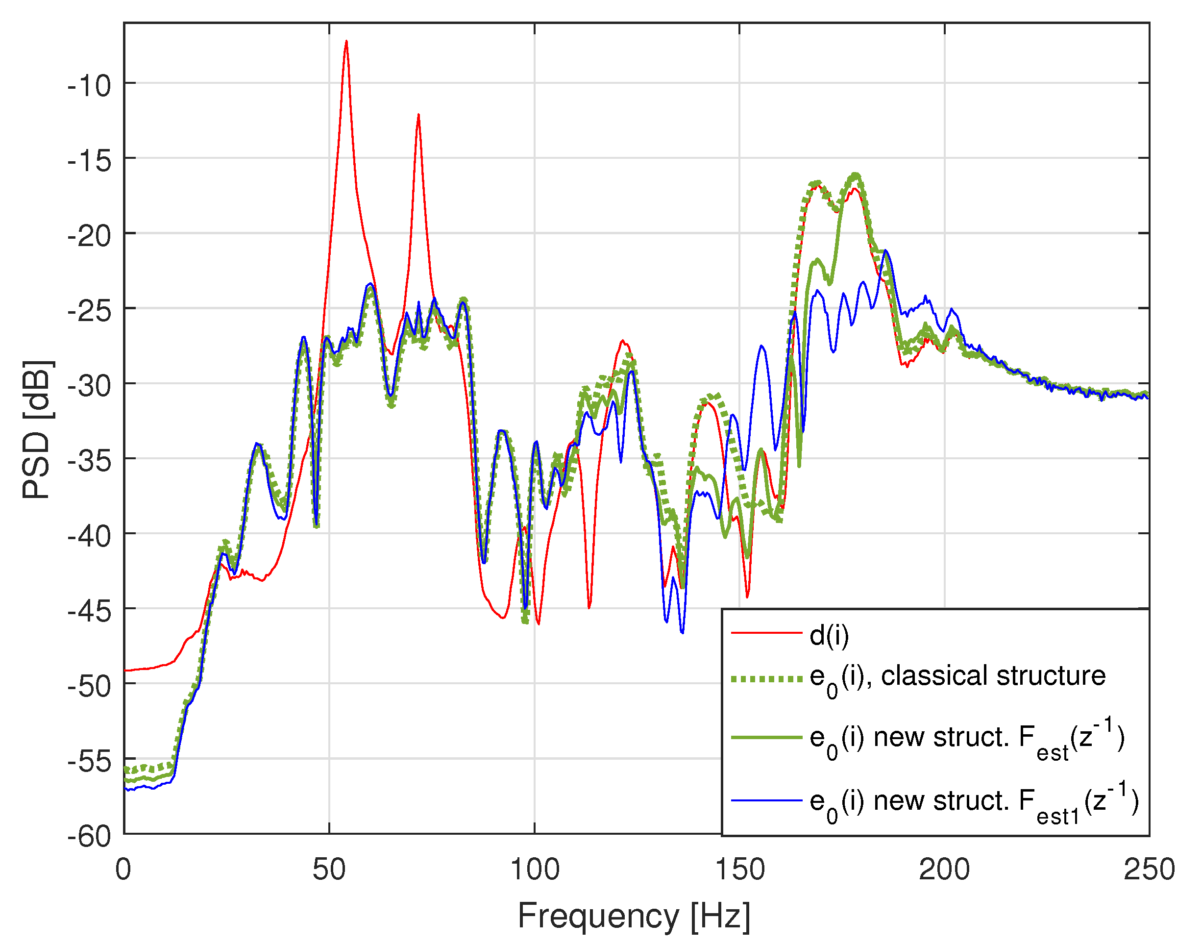
In Figure 21, the estimated power spectral densities of the signals at the error microphone in the new FeFxLMS control system structure with old $F_{est}\left(z^{-1}\right)$ and newly designed filter $F_{est1}\left(z^{-1}\right)$ and the classical FxLMS control system structure are presented. They were obtained for a single realization of the noise to be attenuated after convergence of the adaptation process. It is worth noting that the frequency domain properties of the filter applied to estimate values of the signal at the error microphone influence on a comfort of the active noise control system users. The new FeFxLMS control system structure with the filter $F_{est1}\left(z^{-1}\right)$, that estimates signal values at the error microphone precisely for a wider band of frequencies than it was possible with the filter $F_{est}\left(z^{-1}\right)$, gives the greatest noise reduction but also amplifies noise at frequencies around 200 Hz more than the remaining active noise control systems considered.

5. Conclusions

In this paper, a new approach to the design of active noise control systems was proposed. It resulted in a new control system structure that is a classical control system equipped with an additional discrete-time filter placed in the error signal measurement path to estimate signal values at the input of this path. The estimated signal values were used for the tuning of a corresponding adaptive filter. The presented discussion was illustrated by simulation case studies that showed the effectiveness of the proposed new active noise control system structure. Its application resulted in faster adaptation and greater unwanted noise attenuation after the initial adaptation phase, regardless of the dynamical properties of the active noise control system plant and spectral properties of the noise attenuated. Although the presented discussion was illustrated by simulation case studies in which a feedforward active noise control systems was applied to create local zones of quiet, it is worth emphasizing that the presented idea may also be applied for other adaptive and non-adaptive active noise control systems as well as other predictors and control systems. It should also be mentioned that the presented idea is also valid for active noise control systems, predictors, and control systems working with a random sampling interval [36].