Performance Evaluation of Autonomous Driving Control Algorithm for a Crawler-Type Agricultural Vehicle Based on Low-Cost Multi-Sensor Fusion Positioning

Abstract

The agriculture sector is currently facing the problems of aging and decreasing skilled labor, meaning that the future direction of agriculture will be a transition to automation and mechanization that can maximize efficiency and decrease costs. Moreover, interest in the development of autonomous agricultural vehicles is increasing due to advances in sensor technology and information and communication technology (ICT). Therefore, an autonomous driving control algorithm using a low-cost global navigation satellite system (GNSS)-real-time kinematic (RTK) module and a low-cost motion sensor module was developed to commercialize an autonomous driving system for a crawler-type agricultural vehicle. Moreover, an autonomous driving control algorithm, including the GNSS-RTK/motion sensor integration algorithm and the path-tracking control algorithm, was proposed. Then, the performance of the proposed algorithm was evaluated based on three trajectories. The Root Mean Square Errors (RMSEs) of the path-following of each trajectory are calculated to be 9, 7, and 7 cm, respectively, and the maximum error is smaller than 30 cm. Thus, it is expected that the proposed algorithm could be used to conduct autonomous driving with about a 10 cm-level of accuracy.

1. Introduction

Globally, many countries are facing constraints on food production due to climate change, aging, and decreasing farming population. For example, as reported in [1], the Korean farm population is predicted to decline by 16.7% from 2015 to 2024 and the percentage of farmers over 65 years of age in the farming population is expected to be 43.8% in 2024. For these reasons, in recent years, demand for the mechanization and automation of agriculture is increasing for efficient agricultural production. In addition, advances in sensor technology and information and communication technology (ICT) are leading to the development of autonomous driving agricultural vehicles. For example, major agricultural machinery manufacturers, such as John Deere, Case IH, Yanmar, and New Holland, developed autonomous driving technology or have a concept/plan to carry it out, and more than 20 of the projects are underway across the world [2,3]. John Deere presented an autonomous tractor, the 8320 model with an autonomous system called “Auto Trac Controller” in 2017 and it was put on the market in Denmark [4]. As a plug and play kit, it could be adapted to non-brand tractors and it can detect the obstacles using a laser scanner. Case IH mentioned the concept of an autonomous tractor using on-board sensors and a video camera in 2016 [5]. It could be operated remotely using a tablet and the tractor can identify the obstacles using on-board sensors and camera. Yammar presented a self-driving robot tractor, “Yanmar Robot Tractor” with precise automatic driving control using a global navigation satellite system (GNSS)-real-time kinematic (RTK) module, and Inertial Measurement Unit (IMU) in 2019 [6]. New Holland designed an autonomous tractor, “NHDrive”, which detects obstacle using a combination of radar, light detection and ranging (LiDAR), and cameras in 2016 [7]. Because there are few people and no obstacles in areas where agricultural machinery is used, the risk of accidents caused by using self-driving agricultural vehicles is low. Therefore, if an autonomous driving agricultural vehicle with a price similar to non-autonomous driving agricultural machinery is developed, it is expected that its utilization in the agricultural field will increase.

Since an autonomous driving agricultural vehicle uses navigational information (i.e., position, velocity, and attitude to control vehicle speed, and steering to follow a specific route), navigation sensors should be equipped for the operation of autonomous driving. A typical navigation sensor is GNSS-RTK, which can provide the position, speed, and heading with an accuracy that is appropriate for autonomous driving. Thus, previous studies dealt with GNSS-RTK-based autonomous driving for agricultural vehicles. For example, O’Connor et al. [8] developed a four-antenna carrier-phase GPS system for guiding a tractor with the line tracking standard deviation below 2.5 cm. Stoll and Kuzbach [9] developed an automatic steering system using GNSS-RTK with a standard deviation of lateral error from 2.5 to 6.9 cm. Gan-Mor et al. [10] applied GNSS-RTK for guiding a tractor and its performance in autonomous driving was evaluated to be centimeter level in terms of lateral accuracy. Han et al. [11] used a low-cost single-frequency GNSS-RTK for the autonomous driving system and the root mean square (RMS) of the path-following error of the developed system was found to be a centimeter-level. As above, GNSS-RTK can provide accurate navigational information in most environments at an affordable price, but GNSS-RTK cannot guarantee continuity and reliability of positioning where the GNSS signal environment is poor, such as an orchard [12]. To overcome this problem and to ensure stable autonomous driving, an autonomous driving system was improved by combining GNSS-RTK as well as a dead reckoning sensor such as inertial measurement unit (IMU), tilt sensor, and gyroscope. Noguchi et al. [13] developed an autonomous driving robot for an agricultural operating environment using GNSS-RTK, a fiber optic gyroscope (FOG) and an IMU. The results showed that the RMS position error of the desired path was less than 3 cm. Takai et al. [14] developed a crawler-type tractor that can be operated autonomously using GNSS-RTK and an IMU. The RMS of lateral error in the navigation tests was shown to be less than 5 cm in straight lines in an open sky field. Xiang et al. [15] reported that an automatically guided rice transplanter that uses GNSS-RTK and IMU showed less than 10 cm and 5 degrees for the lateral and heading errors respectively, in straight lines. The summary of previous studies using navigation sensors is summarized in

Table 1. Summary of previous studies using navigation sensors.

Reference.	Sensor	Target Vehicle	Error	Country
O’Connor et al. [8]	4 antenna carrier-phase GPS System	tractor	Less than 2.5 cm	United States
Stoll and Kuzbach [9]	GNSS-RTK	Automatic steering system	2.5–6.9 cm	Germany
Gan-Mor et al. [10]	GNSS-RTK	tractor	Centimeters	Israel
Han et al. [11]	single-frequency GNSS-RTK	speed sprayer	Centimeters	Korea
Noguchi et al. [13]	GNSS-RTK, a fiber optic gyroscope (FOG) and an IMU	autonomous driving robot	3 cm	Japan
Takai et al. [14]	GNSS-RTK and an IMU	crawler-type tractor	5 cm	Japan
Xiang et al. [15]	GNSS-RTK and IMU	rice transplanter	Less than 10 cm	China

.

Recently, advances in micro electromechanical system (MEMS) technology have led to the development of a small and inexpensive MEMS-IMU, and the performance of the MEMS-IMU is being improved [16]. In addition, the performance of a low-cost GNSS-RTK module is improving due to advances in the multi-GNSS positioning technique using GPS, a global navigation satellite system (GLONASS), BeiDou, Galileo, and a quasi-zenith satellite system (QZSS). Despite the development of various sensors, a low-cost autonomous driving system is not yet commercially available because most of the previous studies were conducted by using expensive GNSS-RTK and IMU. Therefore, an autonomous driving algorithm using the fusion of a low-cost GNSS-RTK module and a low-cost motion sensor module was proposed in this study to commercialize a low-cost autonomous driving system for crawler-type agricultural vehicles, and its performance was evaluated based on three different trajectories.

2. Autonomous Driving Control Algorithm

This section presents the proposed autonomous driving control algorithm for the crawler-type agricultural vehicle with a chassis and a working machine attached to one body, such as speed sprayer and weeding vehicle. The algorithm is divided into two parts; one is a GNSS-RTK/motion sensor integrated positioning algorithm, which is used to calculate the navigational information, and the other one, the path-tracking control algorithm, calculates the desired vehicle course based on the vehicle position and waypoints.

2.1. GNSS-RTK/Motion Sensor Integrated Positioning Algorithm

In autonomous driving of the crawler-type vehicle, the left and right track speeds are controlled to follow a specific route based on navigation information and waypoints. Therefore, a GNSS-RTK and a motion sensor integrated positioning algorithm was implemented to guarantee continuity of navigational information and accuracy and stability of autonomous driving. The GNSS-RTK/motion sensor integrated positioning algorithm was implemented by a loosely coupled integration based on an extended Kalman filter (EKF). A block diagram of the GNSS-RTK/motion sensor integrated positioning algorithm is shown in Figure 1. Since the proposed positioning algorithm is similar to the multi-sensor integration algorithm previously studied, please refer to [17,18,19,20,21].

When the accelerometer and gyroscope in the motion sensor measure specific forces and angular rates, respectively, the navigation solutions including position, velocity, and attitude are computed using the inertial navigation system (INS) mechanization (Figure 2). Moreover, the magnetometer in a motion sensor measures both the sign and the magnitude of the earth’s magnetic field, and yaw is calculated by using the current position, attitude, and magnetic declination data and updated in EKF. The process of yaw computation using the magnetometers’ measurement is composed of four parts: (1) tilt compensation to obtain horizontal magnetic measurements, (2) ferrous distortion compensation, (3) magnetic yaw computation, (4) declination angle compensation to adjust the true north. For details of INS mechanization and yaw computation, please see [17,18,19] and [20], respectively. In addition, if the GNSS-RTK module provides the position and velocity information, the GNSS update in EKF is carried out.

In the EKF-based GNSS-RTK/motion sensor integrated positioning algorithm, the error state vector of the navigation part is composed of position errors ($\delta \phi ,$ $\delta \lambda ,$ $\delta h$) expressed in the world geodetic system 1984 (WGS84) coordinate system, velocity errors ($\delta v_n,$ $\delta v_e,$ $\delta v_d$) in the navigation frame, and attitude errors ($\delta \varphi ,$ $\delta \theta ,$ $\delta \psi$). The error state vector of the sensor part consists of accelerometer bias ($\delta b_x,$ $\delta b_y,$ $\delta b_z$) and gyro bias ($\delta d_x,$ $\delta d_y,$ $\delta d_z$), defined by the first-order Gauss–Markov processes. The dynamic model is expressed as:

$$\delta \dot{x}=F\delta x+Gu,$$

(1)

where $F$ is the dynamic matrix, $\delta x$ is the error state vector, $G$ is the shaping matrix, and $u$ is the white noise vector. Details about the dynamic matrix, the shaping matrix, and the white noise vector can be found in [21].

The measurement model is generally written as:

$$z=H\delta x+w_m,$$

(2)

where $z$ is the measurement vector, $H$ is the design matrix, and $w_m$ is the measurement noise vector.

The measurement vector for GNSS ($z_{GNSS}$) is the difference in the position and velocity estimated from the INS mechanization and the data acquired from the GNSS-RTK module, as expressed in (3):

$$z_{GNSS}={\left[\begin{array}{c}\phi \\ \lambda \\ h\\ v_n\\ v_e\\ v_d\end{array}\right]}_{INS}-{\left[\begin{array}{c}{\phi }_{GNSS}\\ {\lambda }_{GNSS}\\ h_{GNSS}\\ C_b^n\left[\begin{array}{c}{V}_{GNSS}\\ 0\\ 0\end{array}\right]\end{array}\right]}_{GNSS},$$

(3)

where the subscripts INS and GNSS denote the value estimates from INS mechanization and the data acquisition of the GNSS-RTK module, respectively; $\phi$, $\lambda$, and $h$ are the latitude, longitude, and ellipsoidal height, respectively; $v_n$, $v_e$, and $v_d$ are the north velocity, east velocity, and down velocity, respectively; $C_b^n$ is the direction cosine matrix from the body frame to the navigation frame; and $V_{GNSS}$ is the speed over the ground provided by the GNSS-RTK module.

The design matrix for GNSS ($H_{GNSS}$) is expressed as:

$$H_{GNSS}=\left[\begin{array}{cccc}{I}_{3\times 3}& 0_{3\times 3}& 0_{3\times 3}& 0_{3\times 6}\\ 0_{3\times 3}& -\left(v_{GNSS}^n\times \right)& 0_{3\times 3}& 0_{3\times 6}\end{array}\right],$$

(4)

where $I_{3\times 3}$ is the 3 × 3 identity matrix, $O_{n\times m}$ is n × m zero matrix, and $v_{GNSS}^n$ is the GNSS derived velocities expressed in the navigation frame.

The measurement vector ($z_{MAG}$) and the design matrix ($H_{MAG}$) based on yaw measurement calculated by using a magnetometer measurement are written as:

$$z_{MAG}={\psi }_{INS}-{\psi }_{MAG},$$

(5)

$$H_{MAG}=\left[\begin{array}{cccc}{0}_{1\times 3}& 0_{1\times 5}& 1& 0_{1\times 6}\end{array}\right],$$

(6)

where the subscript MAG denotes the value calculated by using the magnetometers’ measurement, and $\psi$ is the yaw angle.

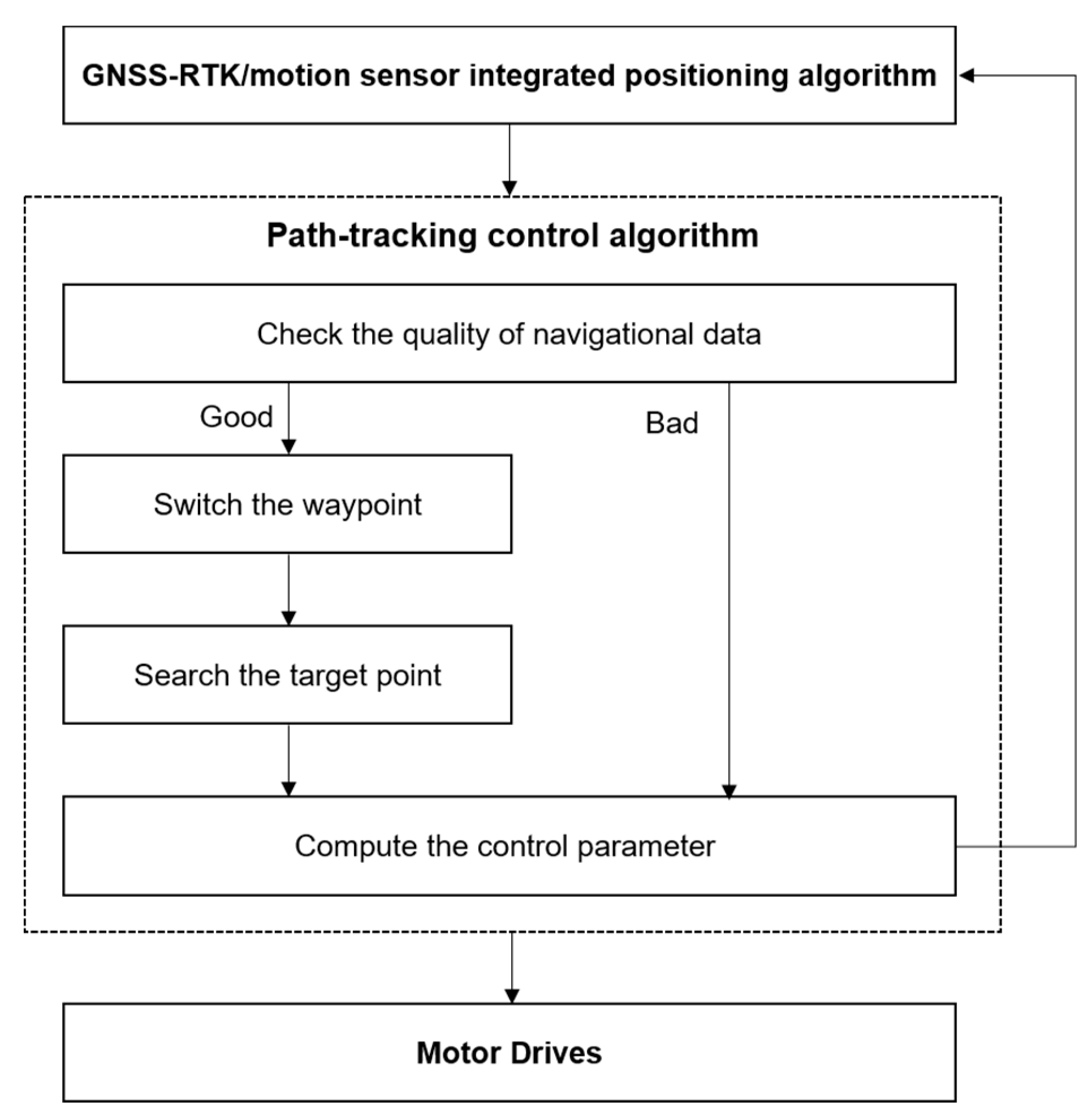
2.2. Path-Tracking Control Algorithm

The path-tracking algorithm computes the control parameters including the left and right track velocities for autonomous driving along the desired vehicle course based on waypoints and the vehicle’s current navigational information. Figure 3 shows the process of the proposed path-tracking control algorithm. The path-tracking control algorithm consists of four parts: checking the quality of navigational data, switching the waypoint, searching the target point, and computing the control parameter. The first step, which checks the quality of navigational data, determines whether to move or to stop an autonomous driving vehicle, as the GNSS-RTK/motion sensor integrated positioning algorithm may provide navigational data of a low quality. In this study, the navigational data are regarded as good quality when the age of the GNSS measurement update with the resolved ambiguity does not exceed 2 s and the precision of position is lower than 0.5 m. If the quality of the navigational data is bad, the left and right track speeds are set to zero and transmitted to the motor drives.

The step of switching the waypoint is to determine whether to switch the next waypoint or not. The route of the vehicle for autonomous driving is represented by waypoints that are a set of points for absolute locations defined by the vehicle’s latitude and longitude coordinates. Since the autonomous driving vehicle navigates between consecutive waypoints, it is important to switch between the various waypoints to follow a specified path. In addition, since the crawler-type vehicle can rotate in-situ, it is necessary to consider whether to rotate in situ or not at the current waypoint. To determine whether the current waypoint is the point of rotation in situ or not, it is necessary to check the angle between the two straight lines created by two adjacent waypoints relative to the current waypoint by the following equation:

$$\left|\mathrm{atan}2\left(\frac{W{P}_{n_{East}}-W{P}_{n-1_{East}}}{W{P}_{n_{North}}-W{P}_{n-1_{North}}}\right)-\mathrm{atan}2\left(\frac{W{P}_{n+1_{East}}-W{P}_{n_{East}}}{W{P}_{n+1_{North}}-W{P}_{n_{North}}}\right)\right|\le \mathsf{\gamma },$$

(7)

where n is the current waypoint index, $W{P}_{n_{North}}$ and $W{P}_{n_{North}}$ are the north and the east coordinates of the current waypoint, which are defined by the north, east, down (NED) relative coordinate system with the origin at the current vehicle’s location, and $\mathsf{\gamma }$ is the reference angle to determine whether to rotate in-situ.

If the current waypoint is the point of rotation, the waypoint is switched when the difference between the current vehicle’s yaw and the azimuth of the straight line generated between the current waypoint and the next waypoint is within the reference angle. If the current waypoint is not the point of rotation in-situ, to switch the next waypoint, it is checked whether the vehicle is within the acceptance radius at the current waypoints, as expressed in the following Equation [22]:

$$W{P}_{n_{North}}^2+W{P}_{n_{East}}^2\le R_{WP}^2,$$

(8)

where $W{P}_{n_{North}}$ and $W{P}_{n_{North}}$ are the north and the east coordinates of the current waypoint, which are defined by the NED relative coordinate system with the origin at the current vehicle’s location, and $R_{WP}$ is the acceptance circle radius for switching the waypoint.

The step of searching the target point is to set a point, which is a location to be moved at the next epoch based on the current vehicle location and the selected waypoint. To set a target point, the enclosed-based line-of-sight (LOS) guidance algorithm [22] is applied in this study. This method is to calculate the coordinates of a target point based on the slope of the straight line between the current waypoint and the previous waypoint and a circle with radius $\mathrm{R}$ enclosing the current vehicle’s location (Figure 4). Details of the equations to calculate the coordinate of a target point using the enclosed-based LOS guidance algorithm can be found in [22]. The difference from the method in [22] is if the distance between the current vehicle’s location and the current waypoint’s location is smaller than radius R, the coordinate of the target point is set to the coordinate of the current waypoint.

In the final step, to compute the control parameter is to calculate the value of the left and right track speed to reach a target point. The method of calculating the control parameters is explained through two cases. The first case is that the vehicle rotates in situ when the distance between the current vehicle’s location and the current waypoint’s location is smaller than radius R. In this case, the same constant value is assigned to the left and the right track speeds, and the sign is assigned differently according to the rotation direction. For example, in the case of a left rotation in situ, the signs of the left and right track speeds are assigned as plus and minus, respectively. In the case of a right rotation in-situ, the signs of the left and right track speeds are assigned as minus and plus, respectively. The second case is for calculating the velocity of the left and right track to drive the vehicle to a target point when the distance between the vehicle’s current location and the current waypoint’s location is larger than radius R. To calculate the velocity of the left and right track, the target angle and the target speed are computed. The target angle (${\alpha }_{TP}$) is the difference between the current vehicle’s yaw and the azimuth of the straight line generated by the vehicle’s current location and the target point’s location, which is calculated by:

$${\alpha }_{TP}=\mathrm{atan}2\left(\frac{T{P}_{East}}{T{P}_{North}}\right)-\psi ,$$

(9)

where $T{P}_{North}$ and $T{P}_{East}$ are the north and the east coordinates of a target point, which are defined by the NED relative coordinate system with the origin at the vehicle’s current location, and $\psi$ is the yaw of the vehicle.

The target speed ($V_{TP}$) is defined based on the target angle as follows:

$$V_{TP}=V_{min}+\left(V_{max}-V_{min}\right)e^{-\frac{{\alpha }_{TP}{}^2}{{\sigma }^2}},$$

(10)

where $V_{min}$ is the lower bound of the speed, $V_{max}$ is the upper bound of the speed, and $\sigma$ is the design parameter to alter the slope of the speed curve.

The velocities of the left and right tracks are calculated as:

$$\left[\begin{array}{c}{v}_{left}\\ v_{right}\end{array}\right]=\left[\begin{array}{cc}1& 1\\ T_r/2& T_r/2\end{array}\right]\left[\begin{array}{c}{V}_{TP}\\ {\alpha }_{TP}/\mathsf{\Delta }t\end{array}\right],$$

(11)

where $v_{left}$ and $v_{right}$ are the left track velocity and the right track velocity, respectively; $T_r$ is the distance between the left track and the right track; and $\mathsf{\Delta }t$ is the control time interval.

3. Performance Evaluation of Autonomous Driving Control Algorithm

3.1. Test Description

The crawler-type vehicle for the autonomous driving test used a speed sprayer prototype, which is created by the Sungboo Industry Company, as shown in Figure 5a.

Table 2. Vehicle specifications.

Item	Contents
Drive system	Crawler
Dimension (length × width × height, mm)	2183 × 1300 × 1241
Engine	48 V AC motor
Crawler Track (length × width × tread, mm)	1100 × 200 × 1100

shows the vehicle’s specifications. The vehicle was equipped with the test hardware for autonomous driving, including a GNSS antenna, a GNSS-RTK module, a motion sensor module, an embedded board, and an LTE communication device (Figure 5b). For the GNSS-RTK module, u-blox ZED-F9P, which provided centimeter-level accuracy GNSS performance based on u-blox multi-band RTK technology [23] is used. The price of the ZED-F9P was about $170. The configuration of the GNSS was set to receive GPS, GLONASS, Galileo, BeiDou and QZSS. The positioning method of the u-blox ZED-F9P was set to the single baseline GNSS RTK mode and the output rate of the GNSS-RTK data was set to 5 Hz. MTi-1, which contained a 3-axis gyroscope, a 3-axis accelerometer, and a 3-axis magnetometer [24], was applied as a motion sensor, and the price was about $150. The output rate of the motion sensor’s raw data was set to 100 Hz. Moreover, an embedded board, the raspberry pi 4 model, was used to operate the autonomous driving control algorithm [25].

The autonomous driving test was conducted to investigate the accuracy of the path-following in a parking lot of the Sungboo Industry Company, where the GNSS signal reception environment is normal. The control interval of the proposed algorithm was set to 0.01 s. Since the speed sprayer runs at a lower speed in spraying pesticides, the maximum and the minimum speed were set at 6 km/h and 0.36 km/h, respectively. The acceptance radius for switching waypoints and the radius for searching a target point were set to 0.4 and 2 m, respectively. The data for generating waypoints was acquired by manually driving a vehicle using a wireless remote controller based on the path-generation algorithm that was developed by [11]. The shape of test paths was defined based on the shape of working paths for the agricultural vehicle, such as a speed sprayer and a weeding vehicle, to which autonomous driving will be applied. In the generation of waypoints, the distance between adjacent points and the angle between successive lines were set to 0.5 m and 3 degrees, respectively. The path-following error for the performance evaluation was calculated as the shortest distance between the vehicle’s location and a straight line between two consecutive waypoints near the vehicle’s location at every epoch (Figure 6). The path-following error ($e$) is calculated as:

$$e=c\sin \theta$$

(12)

$$\theta ={\cos }^{-1}\left(\frac{c^2+a^2-b^2}{2ca}\right)$$

(13)

where $a$ is the distance between two consecutive waypoints near the vehicle’s location, $b$ and $c$ are the distance between the vehicle’s location and the waypoint near the vehicle’s location.

3.2. Performance Evaluation

Three trajectories were used in the performance evaluation of the autonomous driving control algorithm. The first trajectory contained 65 waypoints, and the length of the first trajectory was 51 m. The first trajectory included three straight-line sections, one curve section, and one in-situ rotation section. In Figure 7a, the blue points are the waypoints and the red points are the vehicle running in the first trajectory. Figure 7b shows a path-following error and the vehicle’s yaw. In the first trajectory, the maximum error of the path-following was calculated to be 0.21 m, and the RMS of the path-following error was 0.09 m. It was found that the error of the in-situ rotation section was higher than that of the other sections, as shown in Figure 7. This result was caused by slip due to vehicle dynamic force when the vehicle stopped in the in-situ rotation section.

Figure 8a,b show the vehicle location with the waypoints for the second trajectory and the path-following error with the vehicle’s yaw, respectively. As seen in Figure 8, the second trajectory is composed of four curved sections and five straight-line sections. The number of waypoints was 90 and the length of the trajectory was 81 m. Compared with the first trajectory, the turning radius was narrower in the curve sections. The RMSE (Root Mean Square Error) of the path-following was 0.07 m. Specifically, the vehicle was following the path well, but the largest path-following error, which was 0.21 m, occurred in the end part of the first curve section. It means that the set radius for searching a target point was not perfectly operated to follow the desired path in the narrower curve section. Therefore, perfectly to operate autonomous driving, it is considered that an algorithm for adjusting the target search distance according to the turning radius should be added through various field tests.

The third trajectory consists of 111 waypoints with a total length of 81 m. The third trajectory includes five straight-line sections, two curve sections, and three in-situ rotation sections. The vehicle location with the waypoints for the third trajectory and the path-following error with the vehicle’s yaw are shown in Figure 9. The maximum error and RMSE of the path-following are 0.29 and 0.07 m, respectively. It can be seen that autonomous driving was operated more precisely in curve sections as the turning radius of curve sections is wider than that of curve sections of the second trajectory. However, because the vehicle cannot be perfectly reached, the rotation in-situ waypoint, the first in-situ rotation section, has incurred the largest error. It is considered that the above problem can be solved by adjusting the acceptance radius for switching waypoint based on the characteristic of waypoints such as stop and go.

Summing up the test results, the RMS of the path-following error at three trajectories was calculated to be 10 cm and the maximum error was also bound smaller than 30 cm. However, numerous performance analysis based on various agricultural environments that are used by the autonomous driving agricultural vehicle is necessary to commercialize an autonomous driving system for a crawler-type agricultural vehicle. Moreover, to improve the stability and accuracy, the upgrade of the algorithm would be carried out as follows, in the future. At various curve paths, it is necessary to add the adjustment of an adaptive search radius for the enclosed-based LOS guidance depending on the turning radius for stable autonomous driving. Adjusting the acceptance radius for switching waypoint based on the characteristic of waypoints such as stop and go will be also added in the proposed algorithm. Finally, to provide stable and accurate navigational information in an agricultural environment, filter tuning for the positioning algorithm will be conducted by considering some constraints and additional integration of the track speeds of the vehicle.

4. Conclusions

In this study, an autonomous driving control algorithm for a crawler-type vehicle has been proposed, and the autonomous driving test was conducted to investigate the accuracy of the path-following for the proposed algorithm. The proposed algorithm is based on the use of a low-cost GNSS-RTK module and a low-cost motion sensor module, which consists of the positioning algorithm and the path-tracking control algorithm. To provide the stable accuracy and continuity of navigation information, the positioning algorithm that integrates the GNSS-RTK module with a motion sensor, including a 3-axis gyroscope, a 3-axis accelerometer, and a 3-axis magnetometer, is loosely implemented through coupled-mode EKF. The path-tracking algorithm calculates the left and the right track velocity for autonomous driving using waypoints and vehicle’s navigational information. The performance evaluation was conducted by using three waypoint-based trajectories that include straight-line sections, curve sections, and in-situ rotation section, in a parking lot. As a result, it was found that the RMS of the path-following error for autonomous driving with respect to three trajectories was smaller than 10 cm, and the maximum path-following error did not exceed 30 cm.

Based on the tests, it could be concluded that the autonomous driving using low-cost navigation sensors is available so that this study might help and apply the commercialization of an autonomous driving agricultural vehicle. In addition, the proposed algorithm can be an alternative solution to complement the limitation of the camera and the laser-scanner-based autonomous driving technique. Although, the autonomous driving control algorithm and the performance of the path-following algorithm with about a 10-cm level of accuracy were demonstrated in this paper; however, the algorithm is necessary to be improved as follows in the future. Since the performance of the path-tracking control algorithm depends on the performance of the GNSS-RTK/motion sensor integrated positioning algorithm, filter tuning, additional constraints, and the integration of the track speeds of the vehicle are necessary to compute stable and accurate navigational information in the agricultural environment. In order to improve the performance of the path-following in the curve section, it is necessary to add an adaptive search radius for the enclosed-based LOS guidance depending on the turning radius at various curve paths. In addition, adjusting the acceptance radius for switching the waypoint based on the characteristic of waypoints such as stop and go is necessary to be added to the proposed algorithm. Finally, since the performance evaluation of the proposed algorithm was conducted only in the parking lot, numerous performance analysis is necessary considering a wide variety of operating conditions, such as terrain and driving environment.

References

1. Korea Rural Economic Institute. Agricultural Outlook 2015; Korea Rural Economic Institute: Naju-si, Korea, 2015; pp. 27–28. [Google Scholar]
2. Alberto-Rodriguez, A.; Neri-Muñoz, M.; Ramos-Fernández, J.C.; Márquez-Vera, M.A.; Ramos-Velasco, L.E.; Díaz-Parra, O.; Hernández-Huerta, E. Review of control on agricultural robot tractors. Int. J. Comb. Optim. Probl. Inform. 2020, 11, 9–20. [Google Scholar]
3. FUTURE FARMING. Available online: https://www.futurefarming.com/Machinery/Articles/2019/11/21-autonomous-tractor-projects-around-the-world-501448E/ (accessed on 30 June 2020).
4. MAQUINAC. Available online: https://maquinac.com/2017/12/john-deere-presenta-tractor-autonomo-mas-potente-la-marca/ (accessed on 30 June 2020).
5. MAQUINAC. Available online: https://maquinac.com/2016/08/case-ih-lanzo-su-primer-tractor-autonomo/ (accessed on 30 June 2020).
6. YANMAR. Available online: https://www.yanmar.com/global/about/technology/technical_review/2019/0403_1.html (accessed on 30 June 2020).
7. NEW HOLLAND ARICULTURE. Available online: https://agriculture.newholland.com/apac/en-nz/about-us/whats-up/news-events/2017/new-holland-nhdrive-concept-autonomous-tractor (accessed on 30 June 2020).
8. O’Connor, M.; Bell, T.; Elkaim, G.; Parkinson, B. Automatic steering of farm vehicles using GPS. In Proceedings of the 3rd international conference on precision agriculture, Minneapolis, MN, USA, 23–26 June 1996. [Google Scholar]
9. Stoll, A.; Kutzbach, H.D. Guidance of a forage harvester with GPS. Precis. Agric. 2000, 2, 281–291. [Google Scholar] [CrossRef]
10. Gan-Mor, S.; Clark, R.L.; Upchurch, B.L. Implement lateral position accuracy under RTK-GPS tractor guidance. Comput. Electron. Agric. 2007, 59, 31–38. [Google Scholar] [CrossRef]
11. Han, J.H.; Park, C.H.; Park, Y.J.; Kwon, J.H. Preliminary Results of the Development of a Single-Frequency GNSS RTK-Based Autonomous Driving System for a Speed Sprayer. J. Sens. 2019, 2019, 4687819. [Google Scholar] [CrossRef] [Green Version]
12. Spangenberg, M. Safe Navigation for Vehicles. Ph.D. Thesis, Toulouse University, Toulouse, France, 2009. [Google Scholar]
13. Noguchi, N.; Reid, J.F.; Zhang, Q.; Will, J.D.; Ishii, K. Development of robot tractor based on RTK-GPS and gyroscope. In Proceedings of the 2001 ASAE Annual Meeting, Sacramento, CA, USA, 29 July–1 August 1998. [Google Scholar]
14. Takai, R.; Yang, L.; Noguchi, N. Development of a crawler-type robot tractor using RTK-GPS and IMU. Eng. Agric. Environ. Food 2014, 7, 143–147. [Google Scholar] [CrossRef]
15. Xiang, Y.; Juan, D.U.; Duanyang, G.; Chengqian, J. Development of an automatically guided rice transplanter using RTK-GNSS and IMU. IFAC-PapersOnLine 2018, 51, 374–378. [Google Scholar]
16. Han, J.H.; Park, C.H.; Hong, C.K.; Kwon, J.H. Performance Analysis of Two-Dimensional Dead Reckoning Based on Vehicle Dynamic Sensors during GNSS Outages. J. Sens. 2017, 2017, 9802610. [Google Scholar] [CrossRef] [Green Version]
17. Jekeli, C. Inertial Navigation Systems with Geodetic Applications; Walter de Gruyter: Berlin, Germany, 2001; pp. 101–138. [Google Scholar]
18. Solimeno, A. Low-Cost INS/GPS Data Fusion with Extended Kalman Filter for Airborne Applications. Master’s Thesis, Universidad Tecnica de Lisboa, Lisbon, Portugal, 2007. [Google Scholar]
19. Shin, E. Accuracy Improvement of Low Cost INS/GPS for Land Applications. Master’s Thesis, The University of Calgary, Alberta Calgary, AB, Canada, 2001. [Google Scholar]
20. Won, D.; Ahn, J.; Sung, S.; Heo, M.; Im, S.H.; Lee, Y.J. Performance improvement of inertial navigation system by using magnetometer with vehicle dynamic constraints. J. Sens. 2015, 2015, 435062. [Google Scholar] [CrossRef] [Green Version]
21. Godha, S.; Cannon, M.E. GPS/MEMS INS integrated system for navigation in urban areas. GPS Solut. 2007, 11, 193–203. [Google Scholar] [CrossRef]
22. Jensen, T.M. Waypoint-Following Guidance Based on Feasibility Algorithms. Master’s Thesis, Norwegian University of Science, Trondheim, Norway, 2011. [Google Scholar]
23. ublox ZED-F9P Module. Available online: https://www.u-blox.com/en/product/zed-f9p-module (accessed on 22 April 2020).
24. Xsens MTi 1-Series. Available online: https://www.xsens.com/products/mti-1-series (accessed on 22 April 2020).
25. Raspberry Pi 4. Available online: https://www.raspberrypi.org/products/raspberry-pi-4-model-b (accessed on 22 April 2020).
Figure 1. Block diagram of a global navigation satellite system (GNSS)-real-time kinematic (-RTK)/motion sensor integrated positioning algorithm.
Applsci 10 04667 g001
Figure 2. Block diagram of inertial navigation system (INS) mechanization (modified from [18]).
Applsci 10 04667 g002
Figure 3. Process of the path-tracking control algorithm.
Applsci 10 04667 g003
Figure 4. Enclosed-based line-of-sight (LOS) guidance principle with radius R [11].
Applsci 10 04667 g004
Figure 5. Vehicle and hardware used for autonomous driving: (a) vehicle; (b) hardware.
Applsci 10 04667 g005
Figure 6. Path-following error.
Applsci 10 04667 g006
Figure 7. Autonomous driving results in the first trajectory: (a) driving path with waypoints; (b) path-following error with the vehicle’s yaw.
Applsci 10 04667 g007
Figure 8. Autonomous driving results in the second trajectory: (a) driving path with waypoints; (b) path-following error with the vehicle’s yaw.
Applsci 10 04667 g008
Figure 9. Autonomous driving results in the third trajectory: (a) driving path with waypoints; (b) path-following error with the vehicle’s yaw.
Applsci 10 04667 g009