Exploiting a Deep Neural Network for Efficient Transmit Power Minimization in a Wireless Powered Communication Network

Abstract

In this paper, we propose a learning-based solution for resource allocation in a wireless powered communication network (WPCN). We provide a study and analysis of a deep neural network (DNN) which can reasonably effectively approximate the iterative optimization algorithm for resource allocation in the WPCN. In this scheme, the deep neural network provides an optimized solution for transmitting power with different channel coefficients. The proposed deep neural network accepts the channel coefficient as an input and outputs minimized power for this channel in the WPCN. The DNN learns the relationship between input and output and gives a fairly accurate approximation for the transmit power optimization iterative algorithm. We exploit the sequential parametric convex approximation (SPCA) iterative algorithm to solve the optimization problem for transmit power in the WPCN. The proposed approach ensures the quality of service (QoS) of the WPCN by managing user throughput and by keeping harvested energy levels above a defined threshold. Through numerical results and simulations, it is verified that the proposed scheme can best approximate the SPCA iterative algorithms with low computational time consumption.

1. Introduction

In recent years, deep machine learning has emerged in many fields of engineering. With the advancements in big data and optimization algorithms and with increased computing resources, deep networks are currently the state-of-the-art technique for different problems, from speech processing to computer vision and online gaming [1]. Deep networks have become one of the most popular research directions and play a significant role in many fields, such as machine translation, speech recognition, image recognition and recommendation systems, etc. Researchers are actively attempting to extend these technologies to other domains, including wireless communication [2]. Many researchers have applied deep learning (DL) techniques to communications systems [2,3,4].

In this paper, we propose a deep learning approach to solve the optimization problem in a wireless powered communication network (WPCN). In the literature, many researchers have already proposed solutions that use numerical optimization to solve signal processing tasks [5,6,7]. Most of the solutions use iterative algorithms that input parameters of the network, such as channel gain or the signal to noise ratio (SNR), and run a number of iterations to find optimized solutions as outputs [8,9]. Iterative algorithms are always costly solutions in terms of their complexity and time parameters, and it is not easy to implement those solutions in a real-world paradigm. Thus, it is necessary to find time and complexity-efficient solutions.

1.1. Deep Learning

Deep learning is an emerging tool in wireless communications to solve numerical optimization problems while addressing time and complexity challenges. It has been proven to be the fastest solution in comparison to the traditional numerical optimization approaches [2]. Deep learning is a process which learns the input and output relation of any signal processing task. Multi-layer neural networks, called deep neural networks (DNN), can be used to approximate a given iterative optimization algorithm. The key idea is to consider the given algorithm as a “black box” and try to learn its input/output relationship by using a deep neural network. A network with several layers can effectively approximate a given algorithm by designing and formulating its internal structure. This can be computationally efficient and can reduce processing time for iterative algorithms as it requires multiple layers of simple operations such as matrix-vector multiplication [10]. A single-layer neural network can also provide an approximation to any function, but the layer may not be large enough and may fail to learn and generalize the model correctly. Thus, in many cases, using deep networks can reduce the number of hidden neurons to approximate a function and provide faster solutions [10,11].

The DNN consists of one input layer, one or more hidden layers and one output layer, as shown in Figure 1.The layers close to the input layer are usually called the lower layers, and the ones close to the output are usually called the upper layers. Every layer except the output layer includes a bias neuron and is fully connected to the next layer. A DNN contains a deep stack of hidden layers that makes the network architecture deep [11]. Each layer consists of neurons, which is where functions take place. The input layer consists of neurons equal to the number of input parameters or the number of features of the system. These neurons give an output from whatever input is fed into them. A DNN mainly describes the mapping of an input vector to an output vector. Hidden layers of DNN are designed to model the mapping of input and output vectors of the system.

Neurons in hidden layers, and the number of hidden layers, are hyperparameters in the DNN, and it is necessary to adjust them for the accurate mapping of inputs and outputs. The output of every lth layer in the hidden layer is

$$q_l=g(w_l{q}_{l-1}+b_l)$$

(1)

where $w_l$ and $b_l$ are the weights and biases of the lth layer, respectively. Learning is the problem of finding the weights, $\mathbf{w}$, within some feasible set that will lead to the output that describes the best mapping of the input; $g(.)$ indicates an activation function that applies to the output of every hidden layer.

1.2. Wireless Powered Communication Network

A wireless powered communication network integrates wireless energy transfer (WET) and wireless information transfer (WIT) in a wireless communications network, which provides a solution to limited battery resources in mobile devices. In the WPCN, an energy provider transmits energy to user terminals on downlink, which then use this energy to transmit information on uplink. It is assumed that the transmitter has a fixed power supply (e.g., a battery), whereas the receiver has no fixed power supply and thus needs to replenish energy via wireless energy harvesting from the received interference and/or signal sent by the transmitter.

When we use the time division duplex (TDD) mode in the WPCN, the total coherence interval is divided into two phases (the downlink energy transfer phase and the uplink information transfer phase) while assuming that the exact channel state information is known. For energy and throughput efficiency, it is necessary to schedule uplink and downlink allocation time so that the required QoS of the WPCN can be achieved. In [5], the author mentioned that throughput and energy are functions of time allocation parameters, and QoS can be achieved only by properly designing these parameters. Moreover, for the efficient usage of available resources by the energy provider and to confirm the QoS of the WPCN, it is also necessary to optimize the transmit power of the energy provider. In [12], Liu et al., provided a study on the joint optimization of transmit power control, of information and energy transfer scheduling and of receiver mode switching for wireless information transfer with energy harvesting. In [13], Cheng et al., jointly optimized power and time allocation for each user in order to achieve proportional fairness while controlling the energy consumption offset for the network at a low level.

1.3. Related Work

In recent work, we found some examples that used a DNN to solve optimization problems in wireless communications. In [10], Sun et al., proposed a DNN scheme for real-time interference management over interference-limited channels. They provided a fairly accurate approximation of a popular algorithm, named weighted minimum mean squared error (WMMSE). In [14], Kang et al., discussed a DL-based scheme to estimate channel parameters for wireless energy transfer. They proposed a deep autoencoder as a solution to learn the channel parameters autonomously at the energy transmitter based on the feedback from the energy receivers. They also proposed an adaptive solution to optimize the pilot signals. The proposed scheme optimized the channel parameter well, in comparison to the Gerchberg–Saxton method. In [15], He et al., proposed learning-based wireless powered secure transmission, in which they exploited the potential of deep learning to maximize the effective secrecy throughput of wireless powered systems. They proved that their proposed schemes were much faster than a conventional exhaustive search scheme proposed in previous research. Lee et al., [16] proposed a convolutional neural network (CNN)-based DNN to control the transmit power in device-to-device communications. They showed that their proposed scheme achieved high spectral efficiency while regulating the interference with low computation time in comparison to other conventional schemes from numerical optimization.

1.4. Main Contribution

In this work, we mainly focus on finding a faster and fairly accurate solution for the resource allocation problem in a WPCN. We utilize the advantages of a deep learning scheme to solve the resource allocation problem in a WPCN. The main contributions of our work are summarized as follows.

• First, we propose a sequential parametric convex approximation (SPCA)-based iterative solution for the transmit power minimization problem in a WPCN. The proposed solution can determine the optimal values for minimum transmit power and allocation of downlink/uplink time for energy and information transmission. We generated a data set for deep learning using this solution.
• Secondly, we propose a learning-based DNN scheme exploiting the training data from the SPCA-based approach. The DNN architecture accepts the channel coefficient as input and gives an optimized solution as output. The proposed DNN is fairly accurate at learning the relationships between the input and output of the WPCN system. The proposed scheme gives fast and fairly accurate results compared to the SPCA-based iterative algorithm.
• The performance of our scheme is verified through simulations and experiments. It is proven that the proposed scheme gives an accurate approximation of a conventional iterative algorithm scheme while managing the time complexity well. Our scheme gives a much faster solution than the conventional iterative algorithm.

The next sections of this paper ARE structured as follows. Section 2 discusses the system model and problem formulation for resource allocation in a WPCN. Section 3 explains the proposed scheme, and Section 4 demonstrates the architecture of the DNN and the generation of training and testing data. Section 5 discusses the results produced by the proposed scheme and verifies the results using simulation. Section 6 concludes this paper.

2. System Model and Problem Formulation

We consider a WPCN system with WET on downlink and WIT on uplink, as discussed in [5]. The network consists of a base station (BS) with a hybrid access point (H-AP) for information and energy to serve the WPCN and K single-antenna users, denoted by $U_k,k=1,2,3,\dots ,K$ as seen in Figure 2. We consider the TDD protocol for transmission, in which channel properties are the same on uplink and downlink. The system has frame-based transmission, as shown in Figure 3, where the total frame length is T seconds, which is equal to A channel coherence time in which channel properties remain constant.

Each frame is divided into two phases, as shown in Figure 3: downlink energy transfer and uplink information transfer. In the downlink phase, the H-AP transmits the energy signal to all users in ${\tau }_{o}T$ seconds, where ${\tau }_o,(0<{\tau }_o<1)$ is normalized to the frame length for generalization. Each $U_k$ harvests energy from the energy signals sent by the H-AP in the downlink phase. In the uplink phase, each $U_k$ utilizes that harvested energy to send the information signal to the H-AP. In Figure 3, ${\tau }_1,{\tau }_2,{\tau }_3,\dots ,{\tau }_k$ are the allocated time slots for every user to transmit information during the uplink phase.

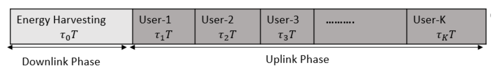
2.1. Downlink Wireless Energy Transfer

In the downlink phase, the H-AP transmits an arbitrary energy signal, $x_A$, where $E\left[\right|x_A{|}^2]=P_A$, in which $P_A$ is the transmit power available to the base station. The received signal by the kth user is $y_k$ defined as

$$y_k=h_k{x}_A+z_k$$

(2)

where $h_k$ is the channel between the H-AP and the kth user, and channel properties remain the same in a coherence interval. Here, $z_k$ is the noise at $U_k$. The amount of energy harvested by the kth user in a downlink can be expressed as $E_k$:

$$E_k={\varsigma }_k{\left|h_k\right|}^2{P}_A{\tau }_0$$

(3)

where $0{<\varsigma }_k<1,k=1,2,3,\dots ,K$ is the energy harvesting efficiency at each receiver.

2.2. Uplink Wireless Information Transfer

After harvesting energy from the H-AP, the kth user sends an information signal utilizing the energy harvested in the downlink phase. Every kth user transmits an independent complex baseband signal, $x_k$. We assume the Gaussian input as $x_k$ is a circularly symmetric complex Gaussian (CSCG) random variable with mean 0 and variance, $\sqrt{P_k}$. We assume that $U_k$ utilizes all the energy harvested on downlink to send the information signal to the H-AP. Thus, $P_k$ denotes the average power at the kth user’s transmitter, which is given by

$$P_k=\frac{E_k}{{\tau }_k},k=1,2,3,\dots K$$

(4)

The received signal at the H-AP sent by the kth user in the kth uplink slot is given by

$$y_{Ak}=h_k{x}_k+z_{A,k}$$

(5)

where $z_{A,k}$ denotes the noise at the H-AP, which is a complex Gaussian-distributed random variable with zero mean and variance, ${\sigma }^2$. The achievable uplink throughput for the kth user in the kth slot can be defined as

$$\begin{array}{cc}\hfill R_k\left(\tau \right)& ={\tau }_k{log}_2\left[1+\frac{{\left|h_k\right|}^2{P}_k}{{\sigma }^2}\right]\hfill \\ \hfill & ={\tau }_k{log}_2\left[1+{\alpha }_k{P}_A\frac{{\tau }_k}{{\tau }_0}\right]\hfill \end{array}$$

(6)

where ${\alpha }_k=\frac{{{{\varsigma }_k|h}_k|}^4}{{\sigma }^2}$. We can see from the above expression that $R_k\left(\tau \right)$ would increase with an increase in transmit power for the given allocated time slots on uplink and downlink. However, as the BS has limited resources and cannot transmit much power to users, there is a need to control the transmit power while maintaining QoS. There is a need to optimize power while maintaining uplink throughput and downlink harvested energy above a specified threshold. Here, we can formulate the problem for transmit power optimization as Equation (7):

$$\begin{array}{cc}\hfill \underset{\tau ,P_A}{min}& P_A\hfill \end{array}$$

(7a)

$$\begin{array}{cc}\hfill \mathrm{s}.\mathrm{t}.& {\tau }_k{log}_2\left[1+{\alpha }_k{P}_A\frac{{\tau }_k}{{\tau }_0}\right]\ge R_{thre}\hfill \end{array}$$

(7b)

$$\begin{array}{cc}\hfill & {\varsigma }_k{\left|h_k\right|}^2{P}_A{\tau }_0\ge E_{thre}\hfill \end{array}$$

(7c)

$$\begin{array}{cc}\hfill & \sum _{j=0}^k{\tau }_j\le 1\hfill \end{array}$$

(7d)

$$\begin{array}{cc}\hfill & {0\le P}_A\le P_{max}\hfill \end{array}$$

(7e)

In Equation (7), we are minimizing the transmit power while optimizing two variables: the transmit power and downlink–uplink time slot allocation. By optimizing these two parameters, we optimize the transmit power. In Equation (7), (7b, and 7c) confirm the QoS while managing uplink throughput and harvested energy to maintain them above threshold levels $R_{thre}$ and $E_{thre}$, respectively. Equation (7d) satisfies the normalization of allocation time based on the frame length. $P_{max}$ is the maximum power resources available at the BS.

However, Equation (7) is a non-convex problem, and it is analytically very difficult to find an optimal solution for $(P^{*},{\tau }^{*})$. Traditionally, non-convex problems can be solved using an exhaustive search algorithm, which requires high computational complexity. For this problem, we propose a deep-learning-based scheme that can give an accurate (and less complex) solution for Equation (7). The analytical results discussed in Section 5 prove this approach to be a promising technique for solving Equation (7) with less computational power compared to traditional approaches.

3. SPCA-Based Iterative Solution

We exploit an SPCA-based iterative algorithm to solve a non-convex problem [17]. For this, we considered Equation (7) in two scenarios for convenience.

3.1. Single User

We consider Equation (7) in a single-user case; i.e., for $K=1$. We can rewrite the Equation (7) as

$$\begin{array}{cc}\hfill \underset{{\tau }_0,P_A}{min}& P_A\hfill \end{array}$$

(8a)

$$\begin{array}{cc}\hfill \mathrm{s}.\mathrm{t}.& 0\ge 2^{R_{thre}/(1-{\tau }_0)}-1-\left({\alpha }_1{P}_A\right)/{\tau }_0-{\alpha }_1{P}_A\hfill \end{array}$$

(8b)

$$\begin{array}{cc}\hfill & 0\ge E_{thre}/{\tau }_0-{\varsigma }_k{\left|h_k\right|}^2{P}_A\hfill \end{array}$$

(8c)

$$\begin{array}{cc}\hfill & 0\le {\tau }_0\le 1\hfill \end{array}$$

(8d)

$$\begin{array}{cc}\hfill & {0\le P}_A\le P_{max}\hfill \end{array}$$

(8e)

This problem is non-convex because of the first constraint, so we need to solve it. Firstly, we convert this non-convex problem to convex sub-problems using sequential parametric convex approximation. After that, the transformed convex problems are solved by the interior point method in a solver such as MATLAB CVX [18,19]. Thus, we converted the above non-convex problem into a convex sub-problem and solved it using the iterative SPCA method in Algorithm 1. This method was used earlier for the energy-harvesting fairness problem in [8]. We set a new variable ${\tilde{P}}_A$, where $P_A={{\tilde{P}}_A}^2$. As we know [19], ${{\tilde{P}}_A}^2$ and $\frac{{{\tilde{P}}_A}^2}{{\tau }_0}$ are convex functions with reference to ${\tilde{P}}_A$ and ${\tau }_0$. At the $n_{t}h$ iteration, we exploit ${{\tilde{P}}_A}^2\ge 2{\tilde{P}}_A^{\left(n\right)}{\tilde{P}}_A-{\tilde{P}}_A^{{\left(n\right)}^2}$ and $\frac{{{\tilde{P}}_A}^2}{{\tau }_0}\ge 2\frac{{\tilde{P}}_A^{\left(n\right)}{\tilde{P}}_A}{{\tau }_0^{\left(n\right)}}-\frac{{\tilde{P}}_A^{\left(n\right)}{\tau }_0}{{\tau }_0^{{\left(n\right)}^2}}$. Thus, we rewrite Equation (8) into a convex sub-problem as,

$$\begin{array}{cc}\hfill \underset{{\tau }_0,{\tilde{P}}_A,s,r}{min}& {{\tilde{P}}_A}^2+s+r\hfill \end{array}$$

(9a)

$$\begin{array}{cc}\hfill \mathrm{s}.\mathrm{t}.& 0\ge 2^{R_{thre}/(1-{\tau }_0)}-1-{\alpha }_1\left[2\frac{{\tilde{P}}_A^{\left(n\right)}{\tilde{P}}_A}{{\tau }_0^{\left(n\right)}}-\frac{{\tilde{P}}_A^{\left(n\right)}{\tau }_0}{{\tau }_0^{{\left(n\right)}^2}}\right]-\hfill \\ \hfill & {\alpha }_1\left[2{\tilde{P}}_A^{\left(n\right)}{\tilde{P}}_A-{\tilde{P}}_A^{{\left(n\right)}^2}\right]-s\hfill \end{array}$$

(9b)

$$\begin{array}{cc}\hfill & 0\ge E_{thre}/{\tau }_0-{\varsigma }_i{\left|h_i\right|}^2\left[2{\tilde{P}}_A^{\left(n\right)}{\tilde{P}}_A-{\tilde{P}}_A^{{\left(n\right)}^2}\right]-r\hfill \end{array}$$

(9c)

$$\begin{array}{cc}\hfill & 0\le {\tau }_0\le 1\hfill \end{array}$$

(9d)

$$\begin{array}{cc}\hfill & 0\le {\tilde{P}}_A\le \sqrt{P_{max}}\hfill \end{array}$$

(9e)

Algorithm 1 Sequential parametric convex approximation (SPCA)-based iterative algorithm to generate data for a single user.

1: initialize: find a feasible point for Equation (9) as initial point $P_A^{\left(0\right)},{{\tau }_0}^{\left(0\right)}$, and find $k^{\left(0\right)}={{P_A}^2}^{\left(0\right)}+s^{\left(0\right)}+r^{\left(0\right)}$ 2: // initial loop: 3: repeat 4: $n\leftarrow n+1$ 5: Solve Equation (9) using CVX and find $P^{*},{{\tau }_0}^{*},k^{*}$ 6: Assign $k^{\left(n\right)}\leftarrow k^{*},{\tilde{P}}_A^{\left(n\right)}\leftarrow {{\tilde{P}}_A}^{*},{{\tau }_0}^{\left(n\right)}\leftarrow {{\tau }_0}^{*}$ 7: until 8: $\frac{\left|k^{\left(n\right)}-k^{\left(n-1\right)}\right|}{k^{\left(n-1\right)}}\le tolerance$ and $s+r\le \epsilon$ 9: // main loop: 10: Generate 10,000 samples for ${P^{\left(n\right)}}^{*},{{{\tau }_0}^{\left(n\right)}}^{*}$ that satisfy Step 7

We generated 10,000 samples for different channel parameters and found optimal values $(P_A^{*},{\tau }_0^{*})$.

3.2. Multiuser

Here, we consider the problem for multi-users. We denote $\mathbf{s}=[s_1,s_2,s_3...,s_k],\mathbf{r}=[r_1,r_2,r_3,...,r_k]$ and $\mathbf{q}=[q_1,q_2,q_3...,q_k]$ as slack variables and rewrite Equation (7) as a non-convex sub-problem that can be solved by using a SPCA based iterative algorithm.

$$\begin{array}{cc}\hfill \underset{P_A,\tau ,\tilde{\tau },s,r,q,t}{min}& {P_A}^2+\sum _{k=1}^K{s}_k+\sum _{k=1}^K{r}_k+\sum _{k=1}^K{q}_k\hfill \end{array}$$

(10a)

$$\begin{array}{cc}\hfill \mathrm{s}.\mathrm{t}.& 0\ge \frac{2^{\frac{R_{thre}}{{\tau }_k}}-1}{{\alpha }_k}-2\frac{P_A^{\left(n\right)}{P}_A}{t^{\left(n\right)}}-\frac{{P_A^{\left(n\right)}}^{2}t}{{t^{\left(n\right)}}^2}-s_k,\forall k\hfill \end{array}$$

(10b)

$$\begin{array}{cc}\hfill & 0\ge \frac{E_{thre}}{1-{\sum }_{k=1}^K\left({\tau }_k\right)}-2{\varsigma }_k{\left|h_k\right|}^2{P}_A^{\left(n\right)}{P}_A-{{\varsigma }_k\left|h_k\right|}^2{P}_A^{{\left(n\right)}^2}-r_k,\forall k\hfill \end{array}$$

(10c)

$$\begin{array}{cc}\hfill & 0\ge \frac{1}{t}-\frac{2}{t^{\left(n\right)}}\sum _{k=1}^K\left({\tilde{\tau }}_k^{\left(n\right)}{\tilde{\tau }}_k\right)+\frac{t}{t^{{\left(n\right)}^2}}\sum _{k=1}^K\left({\tilde{\tau }}_k^{{\left(n\right)}^2}\right)-q_k,\forall k\hfill \end{array}$$

(10d)

$$\begin{array}{cc}\hfill & {0\le P}_A\le \sqrt{P_{max}}\hfill \end{array}$$

(10e)

This problem is very complex to solve in MATLAB CVX with an increasing number of users, and it becomes difficult to solve with the traditional method, whereas the DNN can solve it with less complexity and less time, which will be discussed in a later section. We solve this problem using Algorithm 2.

Algorithm 2 SPCA-based iterative algorithm to generate data for multiple users.

1: initialize: Find a feasible point for Equation (10) as an initial point $P^{\left(0\right)},{\tau }^{\left(0\right)},{\tilde{\tau }}^{\left(0\right)},t^{\left(0\right)}$ and find $k^{\left(0\right)}=P_A^{{\left(0\right)}^2}+{\sum }_{k=1}^K{s}_k^{\left(0\right)}+{\sum }_{k=1}^K{r}_k^{\left(0\right)}+{\sum }_{k=1}^K{q}_k^{\left(0\right)}$ 2: // initial loop: 3: repeat 4: Solve Equation (10) using CVX and find $P_A^{*},{\tau }^{*},{\tilde{\tau }}^{*},t^{*},k^{*}$ 5: Assign $k^{\left(n\right)}\leftarrow k^{*},P_A^{\left(n\right)}\leftarrow P_A^{*},{\tau }^{\left(n\right)}\leftarrow {\tau }^{*},{\tilde{\tau }}^{\left(n\right)}\leftarrow {\tilde{\tau }}^{*},t^{\left(n\right)}\leftarrow t^{*}$ 6: until 7: $\frac{\left|k^{\left(n\right)}-k^{\left(n-1\right)}\right|}{k^{\left(n-1\right)}}\le tolerance$ and ${\sum }_{k=1}^K{s}_k+{\sum }_{k=1}^K{r}_k+{\sum }_{k=1}^K{q}_k\le \epsilon$ 8: // main loop: 9: Generate 10,000 samples for ${P^{\left(n\right)}}^{*},{{\tau }^{\left(n\right)}}^{*}$ that satisfy Step 7

4. Proposed Learning-Based Optimization Scheme

We propose a supervised learning-based deep neural network that learns the non-linear mapping of channel parameter $|h_k|$ to an optimal solution for transmit power and uplink/downlink allocation time $(P^{*},{\tau }^{*})$ where ${\tau }^{*}=[{\tau }_0^{*},{\tau }_1^{*},{\tau }_2^{*}\dots {\tau }_k^{*}]$.

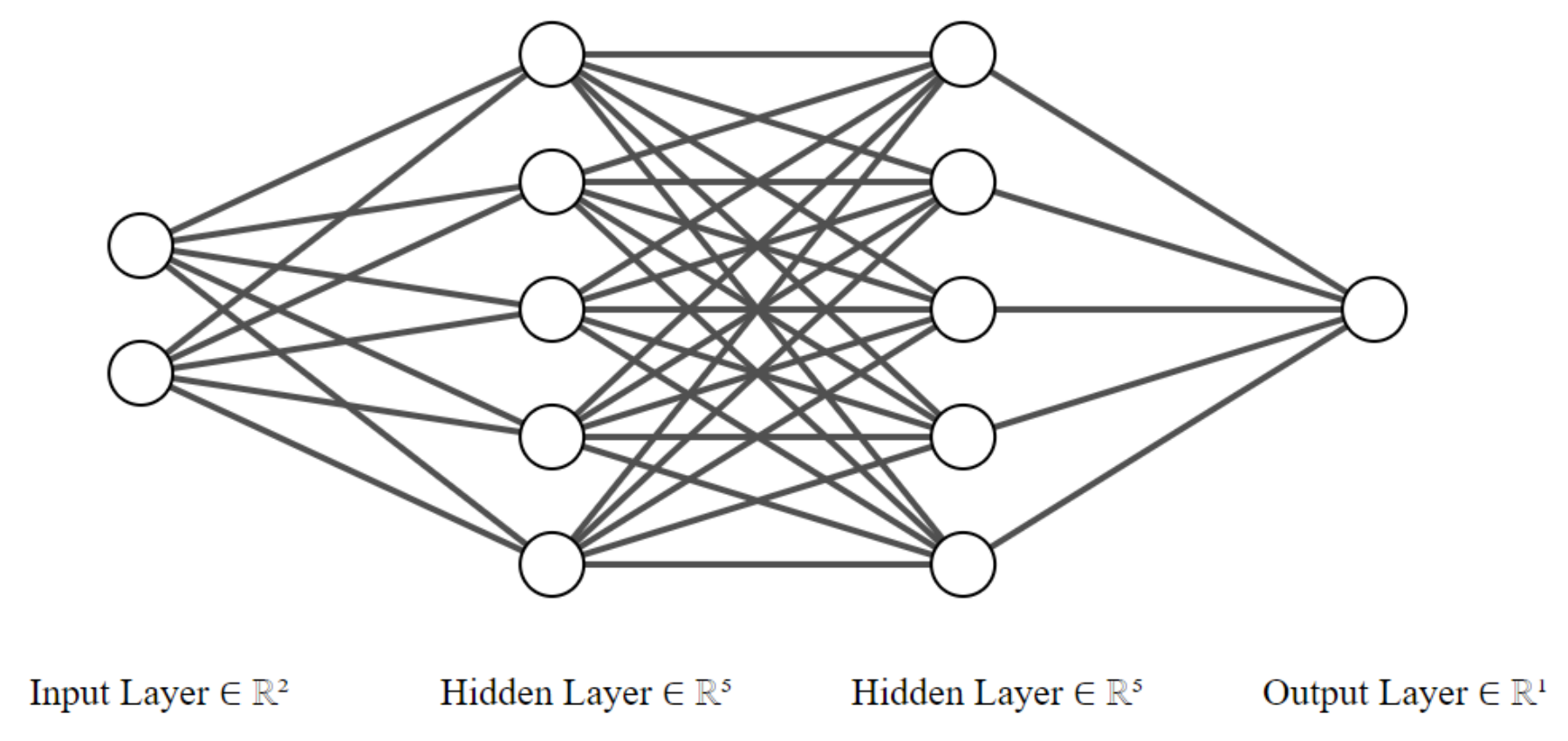
4.1. DNN Architecture

The structure of the proposed neural network consists of a basic multilayer perceptron (MLP). An MLP is a fully connected neural network that consists of one input layer, multiple hidden layers and one output layer. We chose the channel parameter $|h_k|$ for $k=1,2,3,\dots ,K$ as the input to the DNN and the optimal solution $(P^{*},{\tau }^{*})$ as the output of the DNN. Thus, neurons in the input layer are equal to the number of users (i.e., K) in the WPCN, while neurons in the output layer are equal to $K+1$. However, neurons in hidden layers and the number of hidden layers are hyperparameters in the DNN, and it is necessary to adjust them to obtain the best accuracy in the optimal solution. The output of every lth layer in the hidden layer can be defined as shown in Equation (1):

$$q_l=g(w_l{q}_{l-1}+b_l)$$

where $w_l$ and $b_l$ are the weights and biases of the lth layer, respectively. Learning is the problem of finding the weights, $\mathbf{w}$, within some feasible set that will lead to the optimal value of $(P,\tau )$. The initialization of the weights of neurons is very important, because the careful initialization of the network can speed up the learning process [20]. We used a truncated normal distributed random variable divided by the square root of the fan-in for each respective layer to initialize the weights of neurons. This method is the recommended initialization for a rectified linear unit (ReLU) activation function in order to avoid the gradient vanishing problem while optimizing the loss function.

Here, $g(.)$ indicates an activation function that applies to the output of every hidden layer. Activation functions add non-linear properties of the mapping function of input and learning variables. A DNN mainly performs the sum of products of inputs and their respective weights and executes activation function $g(.)$, which is generated for every hidden layer output. An activation function mainly helps the network to learn non-linear complex mapping functions for the input and output. In the proposed scheme, we use the ReLU activation function for the output of every hidden layer. The ReLU in deep networks is easier to optimize, converges faster and is faster to compute [10,14]. ReLU activation function outputs $g\left(x\right)=max(0,x),i.e.,ifx<0,g\left(x\right)=0otherwiseg\left(x\right)=x$.

Thus, the DNN architecture is a function $f(.)$, parameterized by $\mathbf{w}$, that learns the mapping relationship between $(P,\tau )$ and $|h_k|$, which is defined as

$$\left(P,\tau \right)=f\left(|h_k|;\mathbf{w}\right)$$

(11)

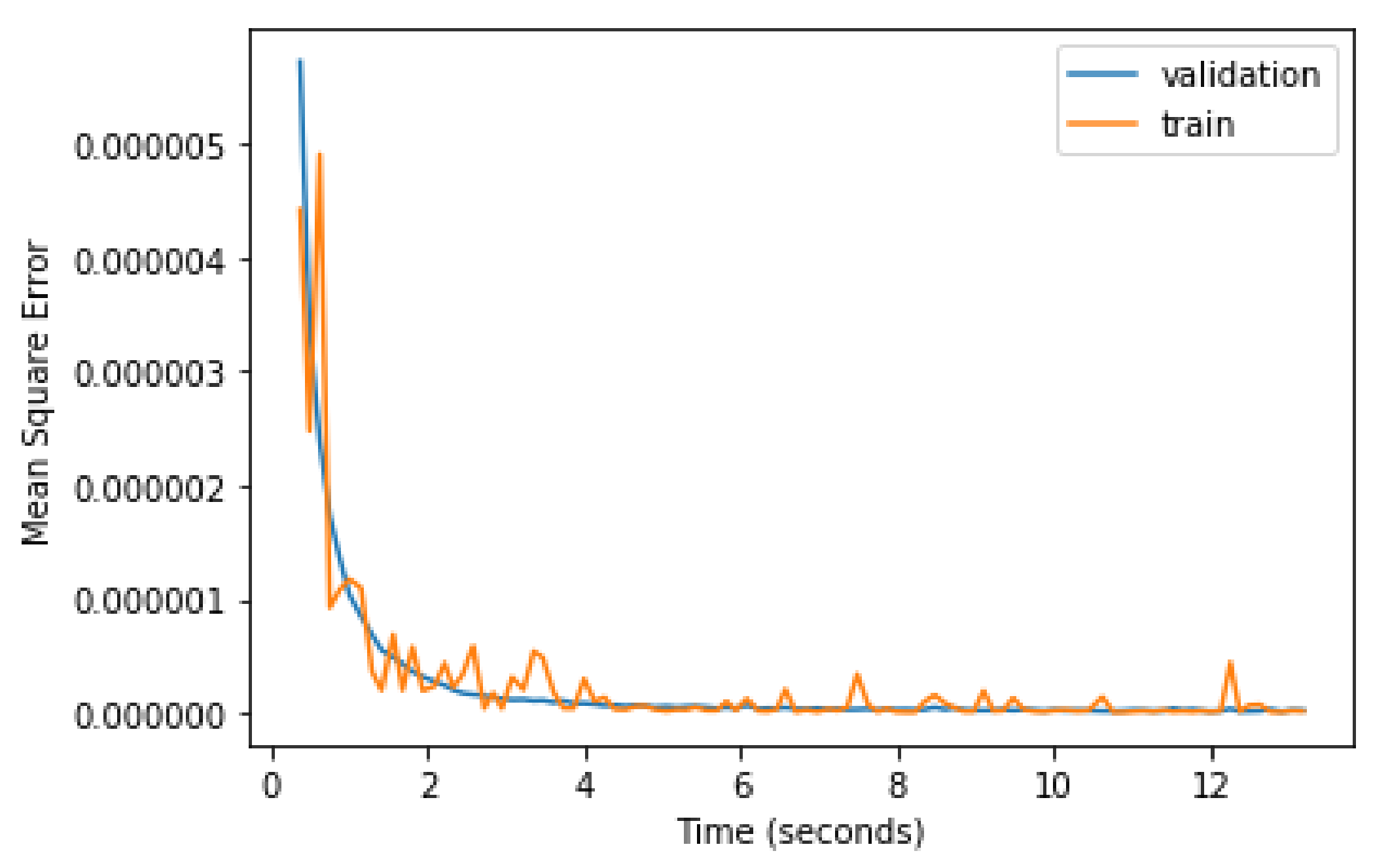
4.2. Training the Neural Network

The training of a neural network is a crucial part of deep learning. A well-trained neural network can learn the mapping between the input and output. In supervised learning, to train a neural network, we need a large number of data samples from the input and output, from which the DNN learns the relationship between the input and output. We trained the neural network with training data that consisted of samples containing $\left(\right|hi|,P^{*},{\tau }^{*})$ generated using the SPCA-based iterative method discussed in the previous section. The training of neural networks is a process to find the network parameter $\mathbf{w}$ by minimizing the loss function. The loss function is basically the difference between the actual $(P^{*},{\tau }^{*})$ from trained data and $(P,\tau )$, the output of the DNN. For this, we consider mean squared error (MSE) as the loss function that should be minimized, so that the output of the DNN, $(P,\tau )$, can approach optimal solution $(P^{*},{\tau }^{*})$. Thus, a well-trained DNN should perfectly minimize the following loss function:

$$J\left(\mathbf{w}\right)=E\left(\right|(P,\tau )-(P^{*},{\tau }^{*}){|}^2)$$

(12)

There are many optimization algorithms which can be used to minimize the loss function. Optimization algorithms compute and update the weights of a network while minimizing the loss function. In our proposed scheme, we used the Adam optimizer to minimize the MSE loss function. The Adam optimizer [21] is a first-order gradient-based optimization algorithm that solves stochastic objective functions with adaptive estimates of lower-order moments. The method is easy to implement, computationally efficient and requires little memory.

There were total $10,000$ data samples available, generated by the SPCA method. We divided all the training samples into three data-sets. We used $60\%$ of the data for training the DNN, $20\%$ for validation and the other $20\%$ for testing. Validation is a process of unbiased evaluation of the network while training the model. The validation of the performance of the DNN model on the training dataset results in a biased score; thus, for unbiased evaluation, we utilized the $20\%$ of dataset for validation that was unknown to the trained model. This was used to determine how well our model learns while training. Testing is a final, unbiased evaluation of the trained model of the neural network. We used data normalization to avoid training and validation errors due to the overfitting problem. After training the DNN, we can utilize it to find the optimal solution for $(P^{*},{\tau }^{*})$ for any new value of channel $|h_k|$.

5. Performance Evaluation

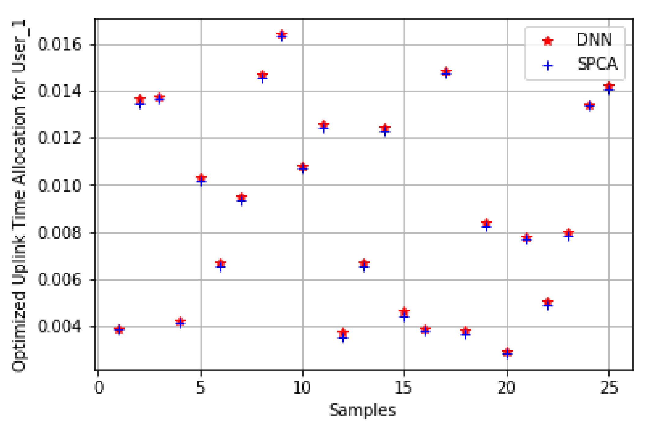
To show the effectiveness of our proposed DNN scheme, we compared the results produced by the DNN with the iterative SPCA method discussed in the previous section. For generating data, we used a Rayleigh fading channel with a noise variance of ${\sigma }^2=-70$ dbm/Hz. The bandwidth was set as 1 MHz. Rayleigh fading is a reasonable channel model that has been widely used to simulate the performance of various resource allocation algorithms [10]. To confirm the QoS of the WPCN, we assumed $R_{thre}$ and $E_{thre}$ to be 1 bit/s/Hz and 1 mW/s, respectively. We considered the receiver efficiency to harvest energy as $0.5$ for each user. We generated $10,000$ samples for both single-user and multi-user scenarios; for multiple users, we consider $K=2$.

5.1. Single User

For $K=1$, we considered a DNN with one input layer, multiple hidden layers and one output layer. There was one neuron in the input layer, where we input the channel parameter $|h_1|$. The output layer consisted of two neurons that represented $(P^{*},{\tau }_0^{*})$. Choosing the number of hidden layers and number of neurons in hidden layers was a crucial part of designing the DNN. We performed experiments for different numbers of hidden layers (i.e., $l=1,2,3,4,5,6$) and different numbers of neurons (i.e., $N=50,100,150,200$). The best and simplest network architecture that we found had three hidden layers with 100 neurons in each hidden layer. We obtained a minimum MSE with less complexity when we chose an architecture with ReLU activation at every hidden layer. We set a batch size of 100 and used 100 training epochs.

We trained the DNN for a single user on 6000 samples and validated the performance on 2000 samples in all training epochs. Figure 4 and Figure 5 show the optimal value for power and downlink-time allocation, respectively, obtained from the DNN and SPCA methods, and show that the DNN achieved the same accuracy with less complexity. Figure 6 shows the MSE convergence for training and validation. This validation performance proves the accuracy of mapping the input and output.

Table 1. Performance evaluation for the deep neural network (DNN) and SPCA method. MSE: mean squared error.

	Single User	Multiple Users
	$\mathit{K}=\mathbf{1}$	$\mathit{K}=\mathbf{2}$
DNN execution time per sample	$5.789\times {10}^{-5}$ s	$5.18\times {10}^{-5}$ s
SPCA execution time per sample	$13.074$ s	$26.993$ s
MSE for optimal power	$1.802\times {10}^{-7}$	$3.67\times {10}^{-9}$
MSE for time allocation	$1.632\times {10}^{-6}$	$5.69\times {10}^{-9}$

, shows that the time required to find the optimal solution to Equation (7) from our proposed scheme is much less than the SPCA method. We performed testing on 2000 data samples, and our proposed scheme obtained an MSE of $1.802\times {10}^{-7}$ for optimal testing power.

5.2. Multi-User

For $K=2$, we considered a DNN with one input layer, three hidden layers and one output layer. There were two neurons in the input layer where we input the channel parameter $|h_k|,k=1,2$. The output layer consisted of three neurons that represented $(P^{*},{\tau }_1^{*},{\tau }_2^{*})$. All hidden layers contained 100 neurons. We set a batch size of 100 and used 100 training epochs. We used the ReLU activation function on the output from every hidden layer. We normalized our data by using a built-in library for prepossessing to avoid training and validation errors due to over-fitting.

Table 1, shows that the time required to find the optimal solution to Equation (7) from our proposed scheme is much less than the SPCA method. Figure 7 shows the optimal value for power obtained from the DNN and SPCA methods. Figure 8 and Figure 9 show the optimal values for uplink time allocation for $U_1$ and $U_2$, respectively. The MSE convergence of validation and training data, as shown in Figure 10 validates the performance of our proposed network. We achieved a low MSE in this case due to normalization. In testing, our proposed scheme obtained an MSE for optimal power of $3.67\times {10}^{-9}$. These results show that the DNN achieved the same accuracy with less complexity.

6. Conclusions

In this paper, we proposed a learning-based wireless powered communication network in which a deep neural network finds solutions for optimized power. The proposed DNN is trained to learn the non-linear mapping between optimal network parameters; i.e., transmit power and uplink/downlink time slot allocation. Training data were generated using an SPCA-based iterative algorithm. The numerical results showed that the performance of the proposed network is fast but has low complexity. We showed that our proposed scheme can achieve the same accuracy as a complex iterative algorithm. Deep learning-based algorithms have great potential in wireless powered communication networks, providing competitive performance with less complexity in comparison with existing solutions.

References

1. Samuel, N.; Diskin, T.; Wiesel, A. Learning to Detect. IEEE Trans. Signal Process. 2019, 67, 2554–2564. [Google Scholar] [CrossRef] [Green Version]
2. Wang, T.; Wen, C.; Wang, H.; Gao, F.; Jiang, T.; Jin, S. Deep learning for wireless physical layer: Opportunities and challenges. China Commun. 2017, 14, 92–111. [Google Scholar] [CrossRef]
3. Farsad, N.; Goldsmith, A. Neural Network Detection of Data Sequences in Communication Systems. IEEE Trans. Signal Process. 2018, 66, 5663–5678. [Google Scholar] [CrossRef] [Green Version]
4. Farsad, N.; Goldsmith, A.J. Detection Algorithms for Communication Systems Using Deep Learning. arXiv 2017, arXiv:1705.08044. [Google Scholar]
5. Ju, H.; Zhang, R. Throughput Maximization in Wireless Powered Communication Networks. IEEE Trans. Wirel. Commun. 2014, 13, 418–428. [Google Scholar] [CrossRef] [Green Version]
6. Yang, G.; Ho, C.K.; Zhang, R.; Guan, Y.L. Throughput Optimization for Massive MIMO Systems Powered by Wireless Energy Transfer. IEEE J. Sel. Areas Commun. 2015, 33, 1640–1650. [Google Scholar] [CrossRef] [Green Version]
7. Li, Q.; Wang, L.; Xu, D. Resource Allocation in Cognitive Wireless Powered Communication Networks under Outage Constraint. In Proceedings of the 2018 IEEE 4th International Conference on Computer and Communications (ICCC), Chengdu, China, 7–10 December 2018; pp. 683–687. [Google Scholar] [CrossRef]
8. Tuan, P.V.; Koo, I. Simultaneous Wireless Information and Power Transfer Solutions for Energy-Harvesting Fairness in Cognitive Multicast Systems. IEICE Trans. Fundam. Electron. Commun. Comput. Sci. 2018, 101, 1988–1992. [Google Scholar] [CrossRef]
9. Tuan, P.V.; Koo, I. Optimizing Efficient Energy Transmission on a SWIPT Interference Channel Under Linear/Nonlinear EH Models. IEEE Syst. J. 2019, 14, 457468. [Google Scholar] [CrossRef]
10. Sun, H.; Chen, X.; Shi, Q.; Hong, M.; Fu, X.; Sidiropoulos, N.D. Learning to Optimize: Training Deep Neural Networks for Interference Management. IEEE Trans. Signal Process. 2018, 66, 5438–5453. [Google Scholar] [CrossRef]
11. Gron, A. Hands-On Machine Learning with Scikit-Learn and TensorFlow: Concepts, Tools, and Techniques to Build Intelligent Systems, 1st ed.; O’Reilly Media, Inc.: Newton, MA, USA, 2017. [Google Scholar]
12. Liu, L.; Zhang, R.; Chua, K. Wireless information transfer with opportunistic energy harvesting. In Proceedings of the 2012 IEEE International Symposium on Information Theory Proceedings, Cambridge, MA, USA, 1–6 July 2012; pp. 950–954. [Google Scholar] [CrossRef] [Green Version]
13. Cheng, Y.; Fu, P.; Chang, Y.; Li, B.; Yuan, X. Joint Power and Time Allocation in Full-Duplex Wireless Powered Communication Networks. Mob. Inf. Syst. 2016, 2016. [Google Scholar] [CrossRef]
14. Kang, J.; Chun, C.; Kim, I. Deep-Learning-Based Channel Estimation for Wireless Energy Transfer. IEEE Commun. Lett. 2018, 22, 2310–2313. [Google Scholar] [CrossRef]
15. He, D.; Liu, C.; Wang, H.; Quek, T.Q.S. Learning-Based Wireless Powered Secure Transmission. IEEE Wirel. Commun. Lett. 2019, 8, 600–603. [Google Scholar] [CrossRef]
16. Lee, W.; Kim, M.; Cho, D. Transmit Power Control Using Deep Neural Network for Underlay Device-to-Device Communication. IEEE Wirel. Commun. Lett. 2019, 8, 141–144. [Google Scholar] [CrossRef]
17. Beck, A.; Ben-Tal, A.; Tetruashvili, L. A sequential parametric convex approximation method with applications to nonconvex truss topology design problems. J. Glob. Optim. 2010, 47, 29–51. [Google Scholar] [CrossRef]
18. Grant, M.; Boyd, S. CVX: Matlab Software for Disciplined Convex Programming, Version 2.1. 2014. Available online: http://cvxr.com/cvx (accessed on 2 July 2020).
19. Boyd, S.; Boyd, S.; Vandenberghe, L.; Press, C.U. Convex Optimization; Berichte über Verteilte Messysteme; Cambridge University Press: Cambridge, UK, 2004. [Google Scholar]
20. Hanin, B.; Rolnick, D. How to start training: The effect of initialization and architecture. In Advances in Neural Information Processing Systems; Curran Associates, Inc.: Montréal, QC, Canada, 2018; pp. 571–581. [Google Scholar]
21. Kingma, D.; Ba, J. Adam: A method for stochastic optimization. arXiv 2014, arXiv:1412.6980. [Google Scholar]
Figure 1. Deep neural network: A fully connected multi-layer neural network that consists of one input layer, two hidden layers and one output layer. Here, R n shows an n-dimensional real number vector.
Applsci 10 04622 g001
Figure 2. A wireless powered communication network (WPCN): A base station with a hybrid access point (H-AP) for energy and information transmission, and K single-antenna users.
Applsci 10 04622 g002
Figure 3. The frame-based WPCN scheme: The total frame is divided into two phases. In the downlink phase, the H-AP transmits an energy signal to all users. The second phase, the uplink phase, shows the allocation of time for each user to send an information signal to the H-AP.
Applsci 10 04622 g003
Figure 4. Optimal power samples from the DNN and SPCA.
Applsci 10 04622 g004
Figure 5. Optimal downlink time allocation samples from the DNN and SPCA.
Applsci 10 04622 g005
Figure 6. MSE convergence for training and validation data in the DNN (single user).
Applsci 10 04622 g006
Figure 7. Optimal power samples from the DNN and SPCA for K = 2 .
Applsci 10 04622 g007
Figure 8. Optimal uplink time allocation samples from the DNN and SPCA for User 1.
Applsci 10 04622 g008
Figure 9. Optimal uplink time allocation samples from the DNN and SPCA for User 2.
Applsci 10 04622 g009
Figure 10. MSE convergence for training and validation data in the DNN (multiple-user).
Applsci 10 04622 g010