Abstract
The Lattice Boltzmann method (LBM) has been applied for the simulation of lid-driven flows inside cavities with internal two-dimensional circular obstacles of various diameters under Reynolds numbers ranging from 100 to 5000. With the LBM, a simplified square cross-sectional cavity was used and a single relaxation time model was employed to simulate complex fluid flow around the obstacles inside the cavity. In order to made better convergence, well-posed boundary conditions should be defined in the domain, such as no-slip conditions on the side and bottom solid-wall surfaces as well as the surface of obstacles and uniform horizontal velocity at the top of the cavity. This study focused on the flow inside a square cavity with internal obstacles with the objective of observing the effect of the Reynolds number and size of the internal obstacles on the flow characteristics and primary/secondary vortex formation. The current LBM has been successfully used to precisely simulate and visualize the primary and secondary vortices inside the cavity. In order to validate the results of this study, the results were compared with existing data. In the case of a cavity without any obstacles, as the Reynolds number increases, the primary vortices move toward the center of the cavity, and the secondary vortices at the bottom corners increase in size. In the case of the cavity with internal obstacles, as the Reynolds number increases, the secondary vortices close to the internal obstacle become smaller owing to the strong primary vortices. In contrast, depending on the sizes of the obstacles ( = 1/16, 1/6, 1/4, and 2/5), secondary vortices are induced at each corner of the cavity and remain stationary, but the secondary vortices close to the top of the obstacle become larger as the size of the obstacle increases.
1. Introduction
In recent years, the Lattice Boltzmann method (LBM) (Guo et al. [1]) has played an important role in resolving a variety of computational engineering problems, particularly incompressible flows (Ghia et al. [2], hereafter GHIA), porous-media flows (Hasert et al. [3]), magneto-hydrodynamics (Chen et al. [4]), and single-phase and multi-phase fluid flows (Yan et al. [5]). LBM is a new approach in the area of computational fluid dynamics (CFD), in which the Reynolds-averaged Navier–Stokes equations (RANS) was originally used for simulating macroscopic quantities of flows (Ghia et al. [2]). LBM comprises the use of the kinetic model with some parameters, and one of them, called the distribution function (Guo et al. [1]), describes the detailed movement and relocation of the fluid particles. These particles are finally located at the lattice nodes through the continuous streaming and collision processes. Furthermore, LBM possesses several distinct merits: it is a simple based on high parallelism, and produces a solution with the complicated boundary condition relatively fast and without transforming the mesh grid (Chang et al. [6]). Moreover, the macroscopic pressure can also be directly solved using the state equation, which provides stable results with a second-order accuracy over a wide range of Reynolds numbers (Re).
The LBM can be divided into two folds, namely the Boltzmann Bhatnagar–Gross–Krook (BGK) model of kinetic theory and the Chapman–Enskog expansion theory. The LBGK method serves as a method for solving continuum problems on a kinetic basis. This method takes into consideration the discrete molecular velocity distribution functions for uniform Cartesian lattices with additional diagonal links. In recent years, the LBGK model has achieved great success in modeling physics in fluids and in viscous flow simulations in a square, two-dimensional cavity driven by a shear layer due to one moving wall for a laminar flow at an up to 10,000. The Chapman–Enskog expansion provides a condition under which hydrodynamics equations for a fluid can be formulated from the Boltzmann equation. This technique justifies the use of various transport coefficients such as thermal conductivity and viscosity, which are important for the transition from a microscopic, particle-based description to a continuum hydro-dynamical and momentum condition. However, the individual molecules are no longer important, and the state of the fluid is described in terms of some average properties of the fluid elements containing billions or much larger numbers of molecules. Therefore, the LBGK model, which was applied in this study, would present more advantages in terms of applicability and domain geometry (i.e., a reasonable running time and boundary condition in complicated geometries). However, there are some limitations to this model. For instance, when the LBGK model runs at a high Re, it runs into the issue of numerical instabilities such that an additional model (such as the MRT model) would be required in some cases.
Lid-driven cavity flow combined with LBM has been one of the benchmark studies in incompressible fluid flow problems. Owing to the simplicity of the geometry under consideration, the reliability and robustness of the governing equations with the incorporated models of the LBM have been thoroughly evaluated in the CFD. However, although it has a relatively simple shape, the internal flow driven by a constant velocity on the lid becomes complicated with the variation of Re, and it forms almost all the phenomena that could possibly exist in incompressible flows: eddies, secondary flows, instabilities, chaotic particle motions, transitions, and turbulence (Shankar and Deshpande [7]). Therefore, this type of flow calculation has been considered as a classic problem and used extensively for the validation of various numerical simulations. In particular, the centerline velocity distributions (i.e., horizontal and vertical centerlines) in a square cavity have been compared with those of benchmark tests and often cited as a benchmark (Ghia et al. [2]).
Erturk et al. [8] simulated a skew cavity flow for two distinct values, i.e., 100 and 1000. Hou et al. [9] studied the effect of compressibility on the lid-driven cavity flow using the Lattice Bhatnagar–Gross–Krook (LBGK) model under an of less than 7500 and using the single relaxation time (SRT) method. They also attempted to investigate the mesh dependence with the objective of determining the time required to arrive at a steady state depending on the lattice size and to observe the Hopf bifurcation at an approximate of 5000 in the cavity flow. In terms of further studies on cavity flows within complex geometries, Aslan et al. [10] compared the stability of the cavity flow for the SRT method with that of the multiple relaxation time (MRT) method with the LBGK model for various values. Lin et al. [11] incorporated the MRT-based LBM for computing lid-driven cavity flows at values ranging from 100 to 7500 and found that it agreed well with existing data for the range of aspect ratios (i.e., the ratio of the depth and width) from 1 to 4. Similarly, GHIA also calculated lid-driven cavity flows with values ranging from 100 to 10,000 using the MRT model. Interestingly, the majority of the existing results were consistent with those of GHIA, which have been used as reference data for lid-driven cavity flows.
In terms of the internal obstacles in the cavity, Su et al. [12] studied the velocity vector plot of lid-driven cavities with multiple obstacles and steady velocity components along the centerline through the cavity for various grid sizes. Gupta and Kalita [13] and Barragy and Carey [14] worked on the cavity flow in other ranges based on a method comprising the stream function and vorticity formulation. Guo et al. [1] designed an LBGK model without the consideration of compressible effects for simulating incompressible flows and that was called the incompressible LBGK model. Bennacer et al. [15] simulated the lid-driven flow with an internal cylinder for a wide range of values. Recently, Kareem and Gao [16] performed a simulation on the flow around a cylinder in a cavity for = 5000, 10,000, 15,000, and 1,330,000 and for a dimensionless rotational speed of the cylinder, . In their study, two different methods—i.e., large eddy simulation and unsteady Reynolds-averaged Navier–Stokes (URANS)—were applied, and the study showed that the flow patterns were strongly influenced on increasing either the rotating cylinder speed or .
Considering the previous studies mentioned above, it can be concluded that there is already (to a great extent) a thorough understanding of lid-driven flows. Additionally, lid-driven cavity flow combined with LBM has been one of the most popular benchmark studies in incompressible fluid flow problems. Therefore, we have focused on a more complex and practical aspect of the lid-driven cavity flow in this study, related to internal obstacles. Although this has wide applicability in medical, thermo-fluid, and industrial sectors, such as heat exchanges, HVAC, and blood flow, we have not found any research on this particular topic in the existing open resources. Regarding the adopted method (i.e., the LBGK model), there are some advantages and limitations. One of its strongest points is that the method was designed to run efficiently on parallel clusters so that it enables complex physics and a sophisticated algorithm. Additionally, the method uses a uniform mesh spacing everywhere in the domain, so that it is usually very fast per time-step. On the other hand, despite the increasing popularity of LBM in simulating complex fluid systems, this method has some limitations. In fact, it requires massive numbers of grid cells (due to uniform resolution) causing ’slow’ overall solution times. In addition, high-Mach number flows in aerodynamics are still difficult for LBM, and a consistent thermo-hydrodynamic scheme is absent.
Additionally, we also aimed in this study to adopt the LBM to observe a lid-driven cavity flow with and without an internal obstacle under number ranging from 100 to 5000. To identify the crucial parameters influencing the flow inside the cavity, our work was focused on observing the detailed flow inside a cavity under a uniform velocity U on the top lid of the cavity. To find the effects of the internal obstacles inside a cavity, four sizes of internal obstacles ( = 1/16, 1/6, 1/4, and 2/5) have been considered. As reported, the flow tends to be stable in the case of a low (i.e., = 100 in our case) and unstable/complicated in the case of a relatively high (i.e., = 5000). Moreover, in this study, an attempt was made to compare our results with the existing data of lid-driven cavity flows, and attention is then focused on the effect of an flow induced around an internal obstacle in a lid-driven cavity.
The rest of this paper is organized as follows. In Section 2, we describe the design of the numerical method used, and thus the lattice Boltzmann governing equation and the boundary condition of the lid-driven cavity are introduced. In Section 3, the results and discussions regarding the flow characteristics of the lid-driven cavity with and without an internal obstacle are presented. In Section 4, we present the core findings and conclusions of this study.
2. Numerical Method
2.1. Governing Equation
In this study, the shape of a cavity considered is a square of size (aspect ratio ), which includes three non-moving no-slip walls and a moving wall () at the top lid having a uniform horizontal velocity. In order to observe the flow instability in the calculation, which was our main concern in this study, values ranging from 100 to 5000 were considered. In order to calculate the cavity flow, the Lattice Boltzmann equation (LBE) was adopted in this study.
The LBE with the BGK collision operator is given as follows:
where and are the discrete distribution function and its equilibrium state, respectively, which form the nine-point integer D2Q9 lattice shown in Figure 1. In addition, is the spatial vector, is the discrete velocity in the ith direction, is the moving index of a particular particle, and is the SRT that manages the rate of distribution function approaching the equilibrium state.
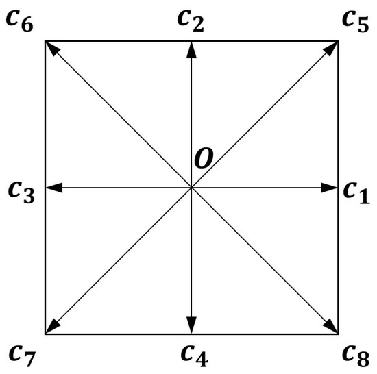
Figure 1.
Schematic of the D2Q9 lattice model.
The equilibrium distribution function can be presented as follows:
In Equation (2), is the weight factor, is the macroscopic velocity, is the density, and p is the pressure, which can be obtained using the following equations:
where is the lattice sound speed. The Chapman–Enskog expansion shows that the LBE satisfies the continuity and momentum equations. The implementation of the controlling equation can be divided into the collision process and streaming process as follows:
In Equations (6) and (7), indicates the post-collision distribution function. In LBM, the relaxation time should be related to the viscosity of the fluid through the Chapman–Enskog expansion in such a manner that the microscopic variables computed from the LBM can satisfy the Navier–Stokes equation with second-order accuracy (Erturk et al. [8]). The relaxation time depends on several variables—the fluid kinematic viscosity , the lattice spacing , the time step , and the density of the fluid , as follows:
where the lattice spacing and time step are set to a unit. In the LBM, there are several lattice models that can be used for the simulation. In the case of a two-dimension domain, the possible directions (i.e., ) in which the particles move would comprise nine different nodes, including the original node (i.e., 0) (D2Q9 model), as shown in Figure 1. When a particle moves and contacts the no-slip wall, it then bounces back in the oncoming direction while retaining its own speed, as shown in Figure 2.
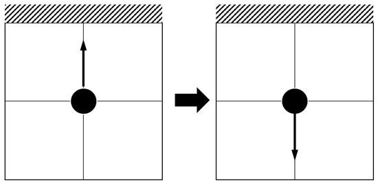
Figure 2.
Schematic of bounce-back boundary condition.
In addition, and in the D2Q9 lattice are represented as follows:
2.2. Boundary Conditions
The simulation of the lid-driven cavity flow has been used as a benchmark for developing the LBM because of its simple shape as well as its extensive application for analyzing complicated flows inside a cavity. This study is aimed at understanding the flow inside a cavity such that it would become important to understand how to implement boundary conditions inside the cavity. No-slip boundary conditions were applied on both the sidewalls and the bottom of the cavity, as well as the obstacle surface, whereas a uniform horizontal velocity (i.e., U = 0.1) was applied at the lid of the cavity, as shown in Figure 3. In Figure 3, the size of each wall is set to the length L (i.e., L = 1). In order to understand the main circulation of the flow inside the cavity, a large circle is used to indicate the primary flow pattern in the cavity.
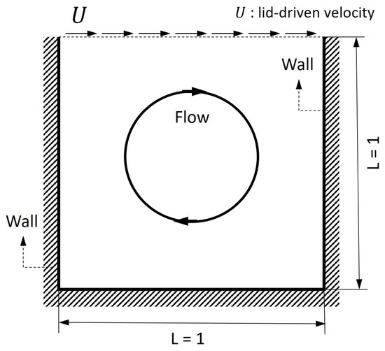
Figure 3.
Schematic of lid-driven cavity flow.
In the case of the flow inside a cavity with an internal obstacle, Figure 4 shows the schematic of lid-driven cavity flow around that internal obstacle. The figure on the left also shows the primary flow pattern indicating the lid-driven flow, as well as a circulating flow around the obstacle. In order to observe the effect of different internal obstacle sizes, the radii of the internal obstacles were varied as = 1/16, 1/6, 1/4, and 2/5.
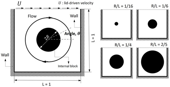
Figure 4.
Schematic of lid-driven cavity flow with internal obstacle of various sizes = 1/16, 1/6, 1/4, and 2/5.
3. Results and Discussion
In this study, the numerical calculation of a two-dimensional lid-driven cavity flow was performed to obtain the solutions for two cases: a cavity flow with and without an obstacle under a range of Reynolds numbers (), and inside the cavity obstacle sizes. In the majority of the cases, a dimensionless cavity , defined as , is applied, where U is the uniform velocity at the top of the cavity, L is the width of the cavity, and is the kinematic viscosity of the fluid. In order to observe the flow inside a cavity, the aspect ratio of the cavity was set as a unit (i.e., a square cavity and L = 1).
In Section 3.1, the mesh dependence check of the cavity flow is presented for the varying the mesh size. In Section 3.2, the observations of the flow inside the cavity without any obstacles and under a range of values are presented with the objective of validating the use of the current methodology for a lid-driven cavity flow. Section 3.3 indicates and validates the locations of the vortex centers in terms of primary and secondary vortices. Finally, Section 3.4 and Section 3.5 present the effect of the internal obstacles on the cavity flow for various obstacle sizes and values.
3.1. Mesh Dependence Check: Mesh Size
In order to determine the dependence of the cavity flow of the mesh size, the simulation was performed at = 2000 with the five meshes sizes of , and , as shown in Figure 5. In order to validate the current LBM model, the results were also compared with the reference data obtained using a commercial software, i.e., ANSYS Fluent. As shown in the figure, the streamlines in the cavity indicate the primary (large circulation in the middle) and secondary (small local circulations in the corner) vortices depending on the mesh size.
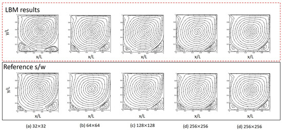
Figure 5.
Mesh dependence check in terms of the size of the grid under the = 2000. The results were compared with those obtained using the commercial software ANSYS Fluent.
Figure 6 shows the vertical distribution of horizontal velocities along the centerlines, with the aim of precisely comparing the velocity components at the centerlines. In each figure, the x and y coordinates depict the corresponding axis, and u and v represent the components of the horizontal and vertical velocities at x = 0.5 and y = 0.5, respectively. To observe the effect of the mesh size, meshes ranging from to were used. As shown in the results obtained using FLUENT, the larger the mesh size, the closer the lines stay to each other. It can be observed in the case of FLUENT, that with a mesh size of , the lines get almost close together. In contrast, the current calculation is almost consistent with the reference data, but there is a discrepancy in the case of the mesh, which appears not to have converged. As shown in Figure 6, the convergence did occur with a mesh size, and thus, taking into consideration the validation of the mesh dependence, a mesh size greater than was used for the rest of this study.
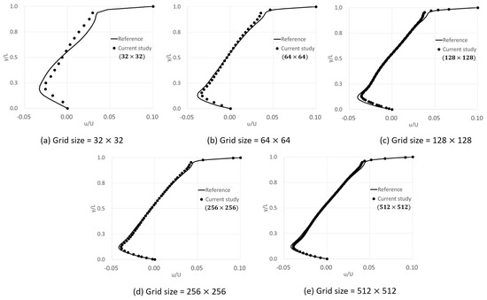
Figure 6.
Vertical distribution of horizontal velocities with various mesh sizes.
3.2. Lid-Driven Square-Cavity Flow without Obstacles
This section describes the variation of the flow inside a lid-driven square cavity without obstacles with the objective of understanding the detailed flow structure inside the cavity. As mentioned earlier, the square-cavity flow would be a well-known benchmark example for validating existing data (Lin et al. [11]). In order to observe the effect of on the flow inside the lid-driven square cavity, the magnitude of the viscosity in is increased by a factor of 50 in order to vary from 100 to 5000, as shown in Figure 7. As increases, the corner vortices gradually appear at the bottom corner of the cavity and become larger. In addition, the center of the primary vortex tends to move to the center of the square cavity. Interestingly, when increases beyond 3000, an induced corner vortex in the upper left corner appears and becomes clearer.
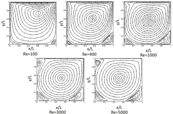
Figure 7.
Streamline distributions with the changing number.
Figure 8 presents the vorticity contours for the changing number. For the figure, the definition of vorticity can be expressed as , where ∇ is the gradient operator (Barragy and Carey [14]). In order to observe the variation of the vorticity strength depending on , in general, the contour line is a curve connecting points where a specific line has the same value. When the lines are close together, the magnitude of the gradient is large, i.e., the variation is steep. As shown in the figure, the strength of the vorticity is evenly distributed inside the cavity except in the region of both top corners at a low number, i.e., = 100 and 400. However, as increases, because of the velocity magnitude of the lid-driven flow, the vorticity center at the top corner moves gradually to the right and right bottom corner, and finally, for = 5000, the strength of the vorticity spreads and dominates all the surrounding edges (due to the thin shear layer close to the wall). In contrast, as increases, the core area in the central region becomes almost constant and fully developed in the range of = 3000–5000.
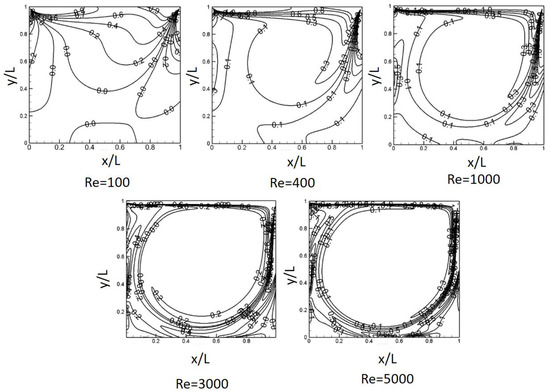
Figure 8.
Vorticity contours for various Re.
Figure 9 shows the two-dimensional vector field inside a square cavity. The length of each vector indicates the flow speed. As shown in Figure 9, in the case of = 100, as the flow looks laminar (i.e., low Reynolds number flow), the center of the primary vortex in the cavity is located in region that is slightly higher, such that the dominant flow would be in the upper region. However, as increases, the primary vortex moves down towards the central region of the cavity and becomes almost axisymmetric in shape.
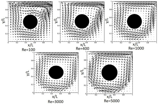
Figure 9.
Vector fields for the changing number.
Figure 10 shows the vertical and horizontal velocity profiles along the centerline of the cavity with the objective of comparing the velocity components precisely with the existing results. In order to observe the effect of on the flow inside the cavity, the was varied from 100 to 5000. In Figure 10a, the velocity distribution shows a positive value at the top region, but a negative-value region below. This indicates that the lid-driven flow naturally exhibits a maximum speed at the lid, which decreases gradually towards the bottom, and changes into a negative velocity in the bottom region due to the circulation of the flow inside the cavity. Interestingly, owing to the no-slip condition at the surface, the maximum negative peak occurs close to the wall, but not at the wall. In addition, the maximum horizontal velocity U varies substantially depending on the number. As increases, the magnitude of the maximum horizontal velocity increases, and the location of the maximum peak point moves towards the wall. As shown in Figure 10b, as increases, the magnitude of the maximum horizontal velocity peak also increases, and the location of the peak point also moves towards the wall. As can be observed from the results, the simulations agree well with the results of an existing study (Ghia et al. [2]).
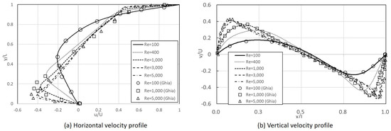
Figure 10.
Vertical and horizontal velocity profiles for various .
3.3. Location of Vortex Centers and Their Comparison
This section describes the locations of the vortex centers formed inside the cavity, such as the left and right bottom vortices and the primary vortices, and a comparison of the current work with the existing work of GHIA is shown in Table 1. In the table, varies from 100 to 5000 and the symbols x, y, and indicate the values in terms of the horizontal and vertical locations and stream function, respectively. In order to analyze the flow variation inside a cavity, the stream function (symbol ) was used to compare the quantity of moving fluid with the existing data (Hou et al. [9]). The stream function has a constant value along each line for a two-dimensional incompressible potential flow. In order to compare the results obtained from stream function, the table lists only the maximum value of stream function (e.g., negative in the case of a counter-clockwise rotation). As shown in the table, compared with the previous work, the locations of the vortex centers obtained in this study have some scatter depending on the location, but the deviation of location (, where and p are the deviation and present value, respectively) is quantitatively a bit higher (around 20%) than those by Bruneau and Saad [17] who obtained the deviations from 4–10% in terms of energy and enstropy for steady lid-driven flow with = 1000 and 5000. Therefore, it should be careful to consider the locations of the vortex center in the table.

Table 1.
Locations of vortices depending on and their comparison with the results of Ghia et al. [2] (GHIA).
3.4. Flow Characteristics inside a Cavity with an Internal Obstacle ( = 1/6)
Figure 11 shows the variation of the flow inside a lid-driven square cavity with obstacles (i.e., = 1/6), with the objective of understanding the characteristics of the flow around obstacles in a lid-driven cavity. In order to perform consistent calculations, is varied from 100 to 5000. As increases, the corner vortex at the bottom gradually appears at the bottom corner of the cavity and becomes larger. In addition, the center of the internal primary vortex tends to move closer to the internal obstacle. However, when exceeds 3000, a corner vortex on the upper left appears and remains there. Interestingly, a large vortex appears around the obstacle at = 100 and becomes a primary vortex. However, as increases, the vortex becomes smaller.
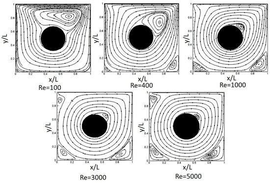
Figure 11.
Streamline distribution with variation in .
Figure 12 shows the vorticity contours for the varying . As shown in the figure, the strength of the vorticity for a smaller stays in the region of the top corners. However, as increases, owing to the lid-driven flow, the strength of the vorticity moves gradually to the right and right bottom corner, and finally, at = 5000, the strength of the vorticity dominates all the surrounding edges (due to the thin shear layer close to the wall). In contrast, the value of central core region shows almost even such that it would have a nearly constant vorticity field. However, the internal obstacle has a substantial influence on the generation of a strong vorticity at a low , but as increases, this influence almost disappears.
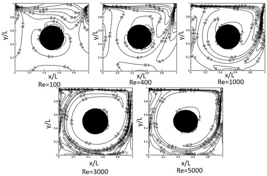
Figure 12.
Vorticity contours for various .
Figure 13 presents the two-dimensional vector field inside the square cavity with an obstacle. The length of each vector indicates the flow speed. As shown in the figure, in the case of = 100, as the flow looks laminar (i.e., a low flow), the vector field in the cavity is slightly erratic, and a circulating flow is observed in the upper region above the obstacle. However, as increases, the upper circulating flow appears to disappear, and a smaller vortex remains at the upper right edge, close to the obstacle, and becomes almost one large circulating flow having a clockwise rotation around the obstacle.
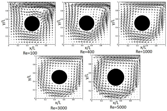
Figure 13.
Vector profiles with the changing .
Figure 14 shows the horizontal and vertical velocity profiles along the centerlines x = 0.5 and y = 0.5. Therefore, the velocity inside the obstacle should be zero in the range of , and . As shown in the Figure 14a, as increases, the magnitude of the negative horizontal velocity in the bottom region increases, and the peak velocity moves lower and close to the wall, whereas the velocity differences in the top region of the cavity are very small, except in the case of a low (i.e., = 100). However, as increases (see Figure 14b), the magnitude of the negative velocity becomes larger, and the peak velocity moves towards the left sidewall, whereas the positive velocity also becomes larger, and the peak velocity moves towards the right sidewall.
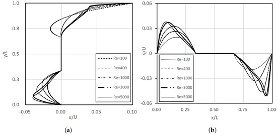
Figure 14.
Vertical (a) and horizontal (b) velocity profiles depending on the number.
3.5. Flow Characteristics inside a Cavity with Varying Sizes of Internal Obstacles ( = 1/16, 1/6, 1/4, and 2/5)
Figure 15 shows the variation of the flow inside the lid-driven square cavity for = 5000 with the radius of the obstacle varying as = 1/16, 1/6, 1/4, and 2/5. As shown in Figure 15, as the size of the obstacle increases, a vortex appears around the obstacles, and it splits into two vortices of different size around the largest obstacle (i.e., = 2/5), which would result in a viscous effect between the obstacle and surface wall of the cavity. In the case of the largest obstacle (i.e., = 2/5), the viscous effect results in an induced vortex in the upper left region around the obstacle.
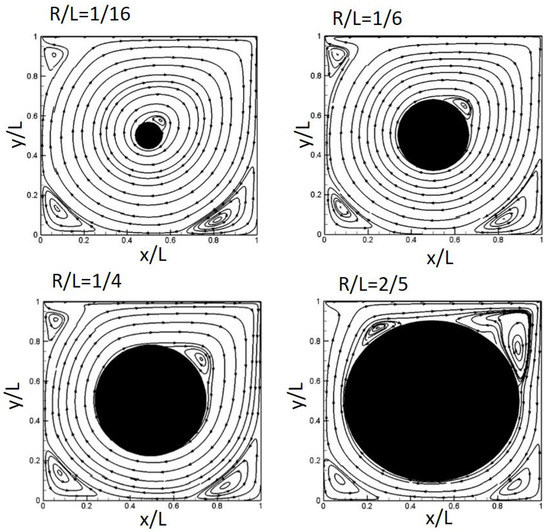
Figure 15.
Streamline distributions for an obstacle of various sizes.
Figure 16 also shows the strength of the vorticity, and depending on the size of the obstacle, dominant vorticity can be shown around the obstacle. The vortex strength is almost similar in all the cases close to the surface wall around the cavity, but the size of the internal obstacle could have a significant effect on the surrounding vorticity.
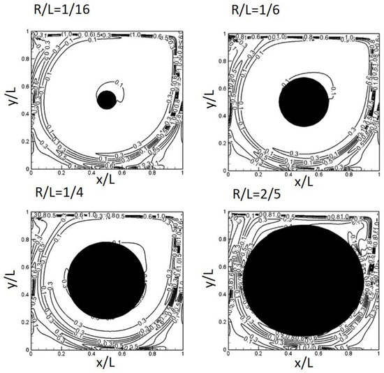
Figure 16.
Vorticity contours for obstacle of various sizes.
Figure 17 shows the two-dimensional vector field inside the square cavity with an of 5000 with obstacles of various sizes ( = 1/16, 1/6, 1/4, and 2/5). As shown in the figure, as the size of the obstacle increases, the vector field does have some effect on the flow around the surface of the cavity wall, but the velocity field in the corner region is only slightly disturbed by the obstacle.
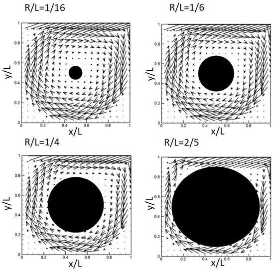
Figure 17.
Vector profiles for obstacles of various sizes.
In order to analyze the velocity variation around the obstacle, Figure 18 shows the speed against the azimuthal angle around the obstacle ( = 1/16, 1/6, 1/4, and 2/5) for the obstacles of various sizes at = 5000 (see Figure 4 for the azimuthal angle). Interestingly, depending on the size of the obstacle, the magnitude of the circumferential velocity shows a significant variation. In the case of = 1/16, the magnitude of the surface velocity () is less than 0.001 in the range of , whereas the other half has a larger magnitude over , which tends to have similar magnitudes in other cases. However, as the size of the obstacle increases, the variation of the circumferential flow varies significantly in the rage of , which could be because the lid-driven flow moves substantially around the obstacle, with a wobbly variation in the lower half of the domain but a smooth flow in the upper half of the domain.
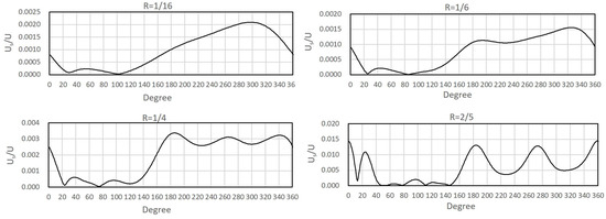
Figure 18.
Flow speed around the obstacle for obstacle of various sizes at = 5000.
4. Conclusions
In this study, the LBGK model has been adopted to simulate the flow inside a two-dimensional cavity and the effect of an internal obstacle under lid-driven cavity flow. For the LBM simulation of lid-driven cavity flow, Reynolds () number varies 100 to 5000 and the aspect ratio of one (i.e., a square cavity, where K = 1). Regarding the LBGK model, one of advantages is that the method was designed to run efficiently on parallel clusters so that it enables complex physics and sophisticated algorithm. In addition, the method uses a uniform mesh spacing everywhere in the domain so that it is usually very fast per time-step. Based on this condition, this study is focused on the LBM for calculating the flow inside a square cavity with and without an internal obstacle depending on number and the size of the internal obstacles. In order to validate the study, the results were thoroughly compared with existing data. The current LBM successfully simulated and used to visualize the precise secondary vortices in the cavity as well as the primary vortex inside the cavity.
The results of this study can be summarized as follows:
- In order to observe the effect of on the flow inside the lid-driven square cavity, the magnitude of the viscosity in is increased by a factor of 50 in order to vary from 100 to 5000. As increases, the primary vortices inside the cavity without an obstacle move towards the center of the cavity, and the secondary vortices at the bottom corners increase in size. However, the core area in the central region is almost constant and fully developed in the range of = 3000–5000.
- In order to analyze the vortex variation inside a cavity, the stream function (symbol ) as well as the locations of the primary and secondary vortices were compared with existing data. The location of the vortex centers obtained in this study have some scatter depending on the location comparing with the previous work, but the deviation of location is, in the majority of cases, less than 20%.
- For the cavity with internal obstacles, as Re number increased, the secondary vortices close to the internal obstacles became smaller owing to the strong primary vortices. Depending on the obstacle size ( = 1/16, 1/6, 1/4, and 2/5), however, secondary vortices were induced at each corner of the cavity and remained stationary, but the secondary vortices close to the top region of the obstacle became larger as the obstacle size was increased.
- In order to analyze the velocity variation around the obstacle, speeds around obstacles of various sizes ( = 1/16, 1/6, 1/4, and 2/5) were compared at = 5000. Interestingly, depending on the size of the obstacle, the magnitude of the circumferential velocity showed a significant variation. In the case of = 1/16, the magnitude of the surface velocity () is less than 0.001 in the range of , whereas the other half has a greater magnitude over , which tends to be similar in the other cases as well.
Author Contributions
Data curation, T.H.; Funding acquisition, H.-C.L.; Project administration, H.-C.L.; Writing original draft, T.H.; Writing review and editing, H.-C.L. All authors have read and agreed to the published version of the manuscript.
Funding
This research received no external funding.
Acknowledgments
This work was supported by ‘Human Resources Program in Energy Technology’ of the Korea Institute of Energy Technology Evaluation and Planning (KETEP), granted financial resource from the Ministry of Trade, Industry and Energy, Republic of Korea (no. 20184030202200). In addition, this work was supported by the National Research Foundation of Korea (NRF) grant funded by the Korea government (MSIP) (no. 2019R1I1A3A01058576).
Conflicts of Interest
The authors declare no conflict of interest.
References
- Guo, Z.L.; Shin, B.C.; Wang, N. Lattice BGK model for incompressible Navier-Stokes equation. J. Comput. Phys. 2000, 165, 288–306. [Google Scholar] [CrossRef]
- Ghia, U.; Ghia, K.N.; Shin, C.T. High-Re solutions for incompressible flow using the Navier-Stokes equations and a multigrid method. J. Comput. Phys. 1982, 48, 387–411. [Google Scholar] [CrossRef]
- Hasert, M.; Bernsdorf, J.; Roller, S. Lattice Boltzmann simulation of non-Darcy flow in porous media. Procedia Comput. Sci. 2011, 4, 1048–1057. [Google Scholar] [CrossRef]
- Chen, S.; Chen, H.; Martinez, D.O.; Matthaeus, W.H. Lattice Boltzmann model for simulation of magnetohydrodynamics. Phys. Rev. Lett. 1991, 67, 3776–3779. [Google Scholar] [CrossRef] [PubMed]
- Yan, Y.Y.; Zu, Y.Q.; Dong, B. LAM, a useful tool for mesoscale modelling of single-phase and multiphase flow. Appl. Therm. Eng. 2011, 31, 649–655. [Google Scholar] [CrossRef]
- Chang, C.; Liu, C.H.; Lin, C.A. Boundary conditions for lattice Boltzmann simulations with complex geometry flows. Comput. Math. Appl. 2009, 58, 940–949. [Google Scholar] [CrossRef]
- Shankar, P.N.; Deshpande, M.D. Fluid Mechanics in the driven cavity. Annu. Rev. Fluid Mech. 2000, 32, 93–136. [Google Scholar] [CrossRef]
- Erturk, E.; Corke, T.; Gokcol, C. Numerical Solutions of 2-D Steady Incompressible Driven Cavity Flow in a driven skewed cavity High Reynolds Numbers. I. J. Numer. Methods Fluids 2005, 48, 747–774. [Google Scholar] [CrossRef]
- Hou, S.; Zhou, Q.; Chen, S.; Doolen, G.; Cogley, A.C. Simulation of cavity flow by the lattice Boltzmann method. J. Comput. Phys. 1995, 118, 329–347. [Google Scholar] [CrossRef]
- Aslan, E.; Taymaz, I.; Benim, A.C. Investigation of the Lattice Boltzmann SRT and MRT Stability for Lid Driven Cavity Flow. J. Mater. Mech. Manuf. 2014, 2, 317–324. [Google Scholar]
- Lin, L.S.; Chen, Y.C.; Lin, C.A. Multi relaxation time lattice Boltzmann simulations of deep lid driven cavity flows at different aspect ratios. Comput. Fluids 2011, 45, 233–240. [Google Scholar] [CrossRef]
- Su, S.W.; Lai, M.C.; Lin, C.A. An immersed boundary technique for simulating complex flows with rigid boundary. Comput. Fluids 2007, 36, 313–324. [Google Scholar] [CrossRef]
- Gupta, M.M.; Kalita, J.C. A new paradigm for solving Navier-stokes equations, streamfunction-velocity formulation. J. Comput. Phys. 2005, 207, 25–68. [Google Scholar] [CrossRef]
- Barragy, E.; Carey, G.F. Stream function-vorticity driven cavity solution using p finite elements. Comput. Fluids 1997, 26, 453–468. [Google Scholar] [CrossRef]
- Bennacer, R.; Reggio, M.; Pellerin, N.; Ma, X.Y. Differentiated heated lid driven cavity interacting with tube a Lattice Boltzmann Study. Therm. Sci. 2017, 21, 89–104. [Google Scholar] [CrossRef]
- Kareem, A.K.; Gao, S. Mixed convection heat transfer of turbulent flow in a three-dimensional lid-driven cavity with a rotating cylinder. I J. Heat Mass Transf. 2017, 112, 185–200. [Google Scholar] [CrossRef]
- Bruneau, C.H.; Saad, M. The 2D lid-driven cavity problem revisited. Comput. Fluids 2006, 35, 326–348. [Google Scholar] [CrossRef]


© 2020 by the authors. Licensee MDPI, Basel, Switzerland. This article is an open access article distributed under the terms and conditions of the Creative Commons Attribution (CC BY) license (http://creativecommons.org/licenses/by/4.0/).