Applying Statistical Analysis and Machine Learning for Modeling the UCS from P-Wave Velocity, Density and Porosity on Dry Travertine

Abstract

In the rock mechanics and rock engineering field, the strength parameter considered to characterize the rock is the uniaxial compressive strength (UCS). It is usually determined in the laboratory through a few statistically representative numbers of specimens, with a recommended minimum of five. The UCS can also be estimated from rock index properties, such as the effective porosity, density, and P-wave velocity. In the case of a porous rock such as travertine, the random distribution of voids inside the test specimen (not detectable in the density-porosity test, but in the compressive strength test) causes large variations on the UCS value, which were found in the range of 62 MPa for this rock. This fact complicates a sufficiently accurate determination of experimental results, also affecting the estimations based on regression analyses. Aiming to solve this problem, statistical analysis, and machine learning models (artificial neural network) was developed to generate a reliable predictive model, through which the best results for a multiple regression model between uniaxial compressive strength (UCS), P-wave velocity and porosity were obtained.

1. Introduction

The uniaxial compressive strength (UCS) is one of the most important parameters used in the rock mechanics and rock engineering field for design. It is widely used to characterize rock [1] and to classify rock masses in a quantitative way [2,3,4]. There are several methods to determine it in the field and in the laboratory, mainly provided by the ISRM Suggested Methods [5,6] and the ASTM [7,8,9] Standard Test Methods.

The determination of UCS in the laboratory can be time-consuming and, in some cases, unaffordable, due to the specimen preparation often requires relatively high-quality cores in order to fulfill geometric and surface specifications, as recommended by the ISRM [5] or ASTM [10]. This may be one of the reasons behind the research of correlations between this parameter and others come from non-destructive methods like P-wave velocity (v_p). The v_p was found to be mainly dependent on multiple factors, with several correlations developed for density (ρ) and porosity (n) [11,12,13,14,15,16]. The UCS depends mainly on ρ and n [17], and therefore on v_p, so many researchers have determined different experimental correlations to indirectly predict the UCS in a more economical way in terms of time and money, thanks to the ultrasonic pulse test [6]. Likewise, rocks are heterogeneous and anisotropic, so an equation that relates UCS with v_p, ρ and n in the same equation, should be more reliable than with each variable separately (95% confidence interval and p-value < 0.05), because, for the same type of rock, there may be variations of these index properties according to its location, as demonstrated by González et al. [18] with saturated limestone.

Another aspect to take into account in the determination of the UCS is the calculation method: (i) the Suggested Methods of the ISRM [5] only indicates that the value of each specimen is reported, while “the number of specimens tested should be determined from practical considerations but at least five are preferred”; (ii) the Standard Test Methods of the ASTM [9,19] indicates that the average value is presented from “the number of specimens necessary to obtain a specific level of statistical results may be determined using Test Method E122”. However, it may not be economically possible to achieve a specific confidence level and professional judgment may be necessary”. In this sense, the calculation commonly performed is the average of the UCS values obtained with each test specimen, while the artificial neural network (ANN) is a much more effective tool in reducing the error of the calculations, especially when the dispersion of the results is high.

The relatively high dispersion of strength results occurs in high-porosity rocks (15–30% according to the International Association of Engineering Geology [20]), where the mechanical behavior is controlled by n [21,22]. ANNs have been applied in rock mechanics and rock engineering to predict the behavior of a rock mass [23], the strength and deformability of intact rock from index properties such as v_p, n, corrected point load index (I_s(50)) and Schmidt’s hammer rebound (R_N) [24,25,26,27,28]. Yilmaz and Yuksek [24] developed predictive models for UCS and elastic modulus (E), adjusting neural network models based on the independent variables Schmidt hammer rebound number, point load index, water content and P-wave speed. Subsequently, the work carried out by Dehghan et al. [25] follows a procedure similar to that of Yilmaz and Yuzek [24], however, it is possible that the neural networks modeled in this work are over-adjusted, since the number of parameters (interactions plus threshold values) of the neural network is greater than the number of samples assigned to the network training process. Then, Rabbani et al. [26] developed the application of a neural network model to predict UCS based on n, bulk density (ρ) and water saturation (S_r), demonstrating the applicability and feasibility of the tool to model the response (validated by the goodness-of-fit indicators) and finally, Barzegar et al. [27] develop a comparative analysis of different machine learning models for the prediction of UCS in travertine rocks, presenting good indicators of goodness of fit, however, in this work, the number of parameters of the neural network model is also greater than number of samples, making it possible that the models developed by Barzegar et al. [27] are over-adjusted.

The aim of this paper is to develop a comparative analysis between conventional statistical fitting methods and the machine learning (ANN) of the UCS of travertine, by means of an experimental correlation between UCS and v_p, ρ_dry and n for a minimum of stress tests in a controlled environment. UCS of travertine rocks is a mechanical process that presents a great dispersion in the results of laboratory tests (62 MPa between the maximum and minimum values), which makes it difficult to fit conventional statistical models. On the other hand, machine learning techniques are effective at modeling nonlinear systems; however, they generally require a larger data set to represent the system to be studied.

2. Materials and Methods

2.1. Specimen Preparation

The studied rock (travertine) comes from a quarry located in Calama, 200 km NE of Antofagasta, capital of the region of Antofagasta, in the north of Chile. Travertine belongs to the Chiu-Chiu Formation, which is between 0.5 and 2.5 Ma in age (Upper Pliocene to Pleistocene age) [29]. Twenty-nine cylindrical specimens with a diameter of 31.1 mm, a height-to-diameter ratio of 2:1 and surface polishing of the basal faces were prepared from different blocks, meeting the ASTM geometric standards for uniaxial compressive strength testing [9] and surface finish and tolerances [10]. All specimens were apparently free of discontinuities and were tested for density, porosity, wave propagation velocities and uniaxial compressive strength.

2.2. Density and Porosity Tests

The 29 cylindrical specimens were tested according to the recommendations made by the ISRM [5] for the determination of dry mass (24 h in the oven at 105 °C) and saturated mass (48 h immersed in water). The submerged mass was calculated by placing the saturated mass on a hydrostatic balance to apply Archimedes’ principle. The dry density (ρ_dry), saturated density (ρ_sat) and porosity (n) are calculated from Equations (1)–(3), respectively:

$${\rho }_{dry}=\frac{m_{dry}}{V_T}=\frac{m_{dry}}{\frac{m_{sat}-m_{sub}}{{\rho }_w}}=\frac{m_{dry}{\rho }_w}{m_{sat}-m_{sub}},$$

(1)

$${\rho }_{sat}=\frac{m_{sat}}{V_T}=\frac{m_{sat}}{\frac{m_{sat}-m_{sub}}{{\rho }_w}}=\frac{m_{sat}{\rho }_w}{m_{sat}-m_{sub}},$$

(2)

$$n=\frac{V_v}{V_T}100=\frac{m_{sat}-m_{dry}}{m_{sat}-m_{sub}}100,$$

(3)

where m_dry is the dry mass (g), m_sat is the saturated mass (g), m_sub is the submerged mass (g), V_v is the pore (void) volume (cm³), V_T is the bulk volume (cm³), and ρ_w is the water density (g·cm⁻³).

2.3. Ultrasonic Pulse Transmission Tests

A PROCEQ Pundit Lab+ apparatus was used to measure primary (v_p) and secondary wave (v_s). velocities. The test specifications are those of the method suggested by the ISRM [6]: 54 kHz bandwidth and direct configuration for the transducer pair (transmitter-receiver). The force applied to the transducers involved a stress less than 10 kPa. The programmed voltage was 500 V and the gain was 1x. The measure of v_p was determined automatically by the machine, and v_s was determined manually when both P and S waves were accoupled in the range of 1.4 to 2.3 times the P-wave time arrival. For good transmission between the transducers, the polished surfaces of the specimens were smeared with stiffer grease.

2.4. Uniaxial Compressive Strength Test

The method suggested by ASTM [9,10] was followed, by using a fully servo-controlled 300 t press (CONTROLS 50-C52Z00 + MCC8 50-C8422/M), which allows uniaxial compression strength tests to be carried out on specimens up to 150 mm in diameter. The loading speed was 0.2 MPa·s⁻¹ so that the test lasted between 5 and 10 min.

2.5. Conventional Statistical Models

The effect of independent variables in the modeling of uniaxial compressive strength was studied by means of an experimental design [30,31] generating multiple linear regression models and a quadratic model, adjusted to the experimental tests to study the strength of travertine to variations of v_p, n and ρ_dry.

The methodology used consisted of compression tests, and 29 experimental tests were carried out, studying the effects of velocity of propagation, saturated density and porosity on the dependent variable. For the modeling and experimental design of regression models, the Python “Scipy” library and “statsmodels” module was used (using the ordinary least squares method), making it possible to investigate the linear effects, interactions and quadratic effects of the independent variables in the UCS. The experimental data were fitted first to a simple (v_p-dependent) regression model, and then through a multiple regression analysis [32] (incorporating n and ρ_dry) to a quadratic model, considering only those factors that help explain the model variability and that have statistical significance (p < significance level).

The general form of the experimental model is presented in Equation (4):

$$Y=b_0+{\displaystyle \sum }_{i=1}^n{b}_i{x}_i+{\displaystyle \sum }_{i=1}^n{\displaystyle \sum }_{j=1}^n{b}_{ij}{x}_i{x}_j$$

(4)

where x_i are the independent variables (v_p, ρ_dry, n), and the answer Y corresponds to the dependent variable (UCS). The determination coefficient (R²), p-values and F-value indicate whether the model obtained is adequate to describe the uniaxial compressive strength for the set of values sampled [33,34].

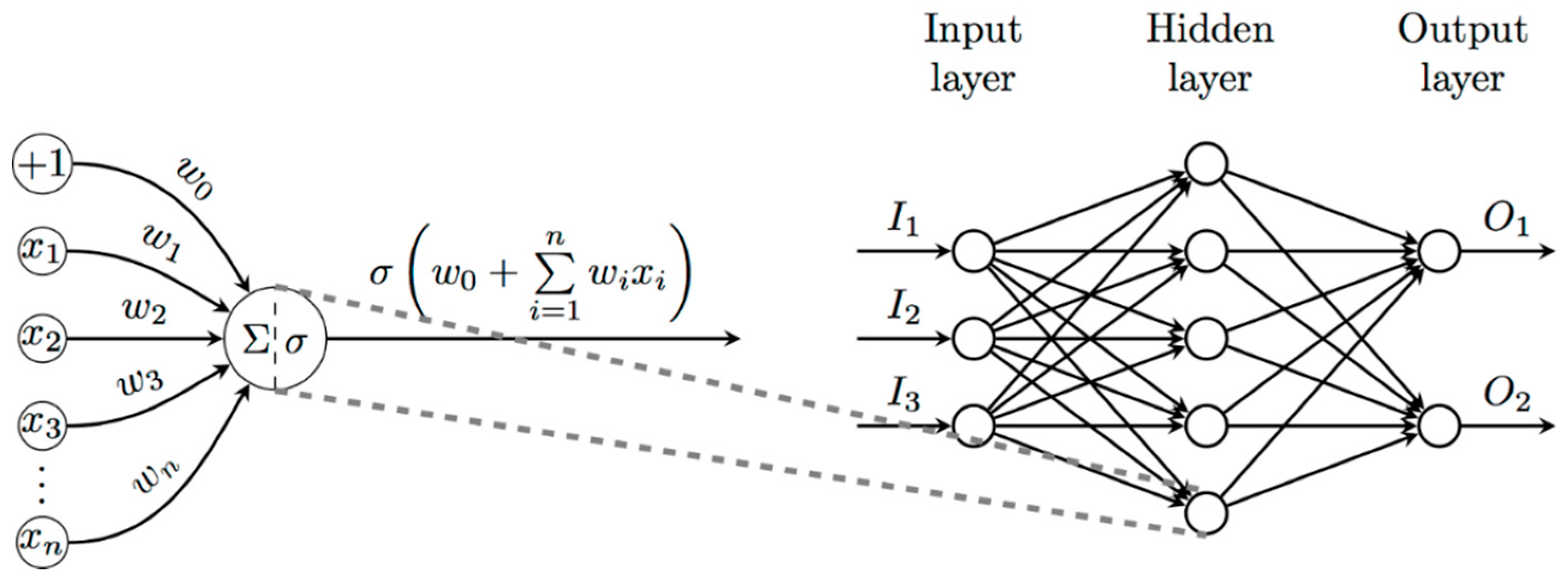
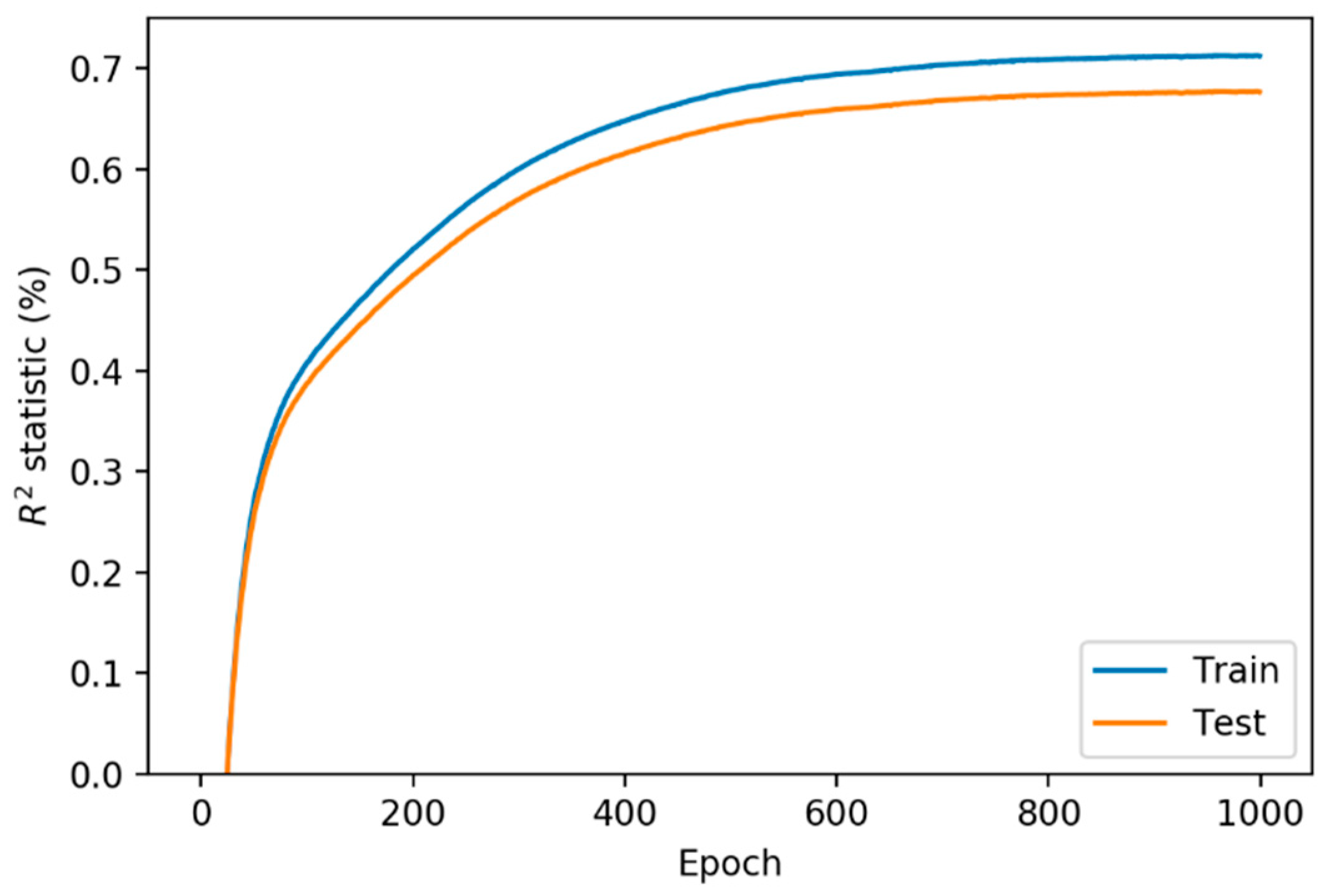
2.6. Artificial Neural Networks

ANNs are supervised machine learning techniques, which determine associations between a known set of observations (i.e., training points) and different environmental variables to classify new and unknown data (test set). ANNs can approximate non-linear relationships and generalize complex systems from relatively imprecise information, and are robust in handling noise, overfittings, and outliers [35].

In an ANN system, the nodes are connected by means of synapses, this connection structure determines the behavior of the network. The most used structure is the multilayer perceptron [36], as presented in Figure 1, where x_i represents the inputs, oi the outputs and σ the activation function. The neurons in the input layer depend on the information available to be classified, which is given by the variables: compression speed, ρ_sat and n, while the output layer is given by the uniaxial compression resistance.

The mathematical expression that describes the output of each neuron is given by the activation function σ, where ω_i, are the synaptic weights that weight the x_i inputs, ω₀ is the threshold and n is the total number of synaptic weights connected to the input of the neuron. Each neuron has its respective threshold level, and the hyperbolic tangent was used as a trigger function on all neurons in the network [37]. The learning method used was backpropagation, which follows the following stages: it starts when a sample of the process is captured by the input layer, then the activation value of each of the neurons is calculated progressively through each neuron or node through all the layers, from the input layer to the output one. Then, in the check stage, the activation value of the output neurons is compared with the expected output data and, if this error differs too much, the error is corrected in a distributed way by updating the weights of the neural network in a return stage, from the output layer to the input one. The whole process is repeated until the network adjusts the synaptic weights and the error value of the outputs is permissible [35].

The implementation of neural network models was developed by generating a model using the Keras neural network library. Keras models are defined as a sequence of layers, for which a “Sequential” model is created, adding layers one after another, until the requirements are met. Then, due to the limited number of samples, the models to be generated are 1 hidden layer, with variations in the number of neurons, which are completely connected by using the dense class. For the hidden layer, the “relu” activation function will be defined, and for the output layer, a “sigmoid” function. Each ANN will be trained for a total of 1000 epochs, the number of neurons in the hidden layer will be defined in the next section, while that median absolute deviation (MAD), mean squared error (MSE), coefficient of determination (R²) and accuracy (ACC) were used to evaluate the fit of the modeled networks. Accuracy is a performance measure defined how the ratio of correctly predicted observation over the total observations.

3. Analysis and Discussion of Results

The results from index properties (v_p, v_s, ρ_dry, ρ_sat and n) and strength (UCS) are shown in

Table 1. Results for geometry, index properties (v_p, v_s, ρ y n) and uniaxial compressive strength (UCS).

Specimen	Diameter, D (mm)	Height, H (mm)	Porosity, n (%)	Density, ρ (g·cm−3)		P-Wave Velocity, vp (km·s−1)		S-Wave Velocity, vs. (km·s−1)		Uniaxial Compressive Strength, UCS (MPa)
				Dry	Sat	Dry	Sat	Dry	Sat
Travertine 1	31.090	59.470	3.65	2.48	2.52	5.310	5.505	3.109	3.030	75.28
Travertine 2	30.970	59.550	4.09	2.37	2.41	5.085	5.505	3.243	3.046	74.95
Travertine 3	31.000	60.350	4.44	2.37	2.41	5.263	5.769	3.279	3.158	89.91
Travertine 4	30.750	60.350	4.58	2.36	2.41	5.263	5.505	3.279	2.943	89.79
Travertine 5	31.050	60.160	5.02	2.38	2.41	4.503	5.505	3.141	3.046	70.12
Travertine 6	31.080	60.310	4.57	2.47	2.51	5.263	5.505	3.226	3.109	78.43
Travertine 7	31.170	59.980	4.70	2.41	2.46	5.263	5.607	3.279	3.158	85.05
Travertine 8	31.118	59.688	4.37	2.48	2.53	5.263	5.882	3.191	3.094	74.79
Travertine 9	31.070	59.780	7.19	2.41	2.48	4.839	5.310	3.125	2.985	78.84
Travertine 10	31.020	59.800	6.65	2.40	2.47	4.839	5.263	3.030	2.985	85.98
Travertine 11	31.175	61.613	4.92	2.47	2.52	4.959	5.439	2.313	2.480	63.78
Travertine 12	31.213	62.450	4.71	2.46	2.51	4.960	5.439	2.375	2.500	95.01
Travertine 13	31.200	62.900	2.98	2.45	2.49	5.167	5.439	2.650	2.520	105.98
Travertine 14	31.200	61.950	4.00	2.41	2.45	4.921	5.439	2.206	2.510	81.91
Travertine 15	31.187	62.000	4.12	2.44	2.48	5.210	5.439	2.403	2.510	94.61
Travertine 16	31.250	61.663	4.61	2.41	2.45	4.960	5.439	2.594	2.520	88.86
Travertine 17	31.163	61.938	8.01	2.34	2.42	4.593	5.000	2.441	2.818	72.65
Travertine 18	31.200	61.950	7.34	2.40	2.47	4.960	5.688	2.296	2.672	70.21
Travertine 19	31.300	62.650	3.43	2.42	2.46	5.391	5.794	2.661	1.981	98.26
Travertine 20	31.250	61.925	3.68	2.45	2.49	5.167	5.439	2.616	2.279	84.71
Travertine 21	31.150	62.450	5.42	2.37	2.43	5.299	5.391	2.520	2.026	81.05
Travertine 22	31.150	62.350	2.32	2.41	2.43	5.391	5.688	2.719	2.780	113.38
Travertine 23	31.220	62.300	4.19	2.37	2.41	5.210	5.487	2.583	2.831	90.77
Travertine 24	31.100	62.650	4.71	2.45	2.50	5.167	5.391	2.627	2.661	88.17
Travertine 25	31.200	62.250	1.05	2.49	2.50	5.688	5.688	2.768	2.756	115.43
Travertine 26	31.400	62.100	0.99	2.47	2.48	5.741	5.487	2.768	2.756	120.17
Travertine 27	31.400	62.200	0.77	2.46	2.46	5.688	5.741	2.793	2.793	115.56
Travertine 28	31.200	62.700	0.72	2.50	2.51	5.688	5.688	2.805	2.793	125.87
Travertine 29	31.250	62.500	0.70	2.43	2.43	5.688	5.794	2.780	2.780	112.87
Maximum	31.400	62.900	8.013	2.503	2.53	5.741	5.882	3.158	3.279	125.87
Minimum	30.750	59.470	0.697	2.342	2.41	4.503	5.000	1.981	2.206	63.78
Mean	31.156	61.447	4.067	2.418	2.47	5.198	5.526	2.742	2.787	90.427
Stand. Dev.	0.1280	1.162	1.940	0.045	0.04	0.316	0.187	0.311	0.337	16.753

. The mean values of ρ_dry, ρ_sat and n were 2.43 g·cm⁻³, 2.47 g·cm⁻³ and 4.05%, respectively. The n values range from 0.7 to 8.1%, a fairly wide interval, due to the heterogeneity in the pore distribution and the travertine petrofabrics [38,39], which is in line with the UCS values, whose average value was 91.72 MPa but in the 25–29 test specimens the UCS values became 70 MPa on average to 120 MPa, coinciding with this decrease in n.

The increase in dry and saturated primary velocity ∆v_p was 369 m·s⁻¹ on average, from which a clay mineral content ECC practically zero, has been deduced [40]. The average dry v_p/v_s ratio is 1.84, within the range 1.8–2 obtained by Soete et al. [38] for travertine and 1.6–2.3 by Schön [41], for consolidated sediments.

The dry v_p values were correlated with the UCS of the rocks using the simple and multivariate regression methods. The experimental data set was used to generate empirical equations developed to estimate the UCS of travertine from the independent variables v_p, ρ_dry and n. In simple regression analyses, models were generated to individually relate the independent variables (v_p, ρ_dry and n) to the dependent one (UCS) by means of simple linear regression models, exponential models, potentials and quadratics through a logarithmic transformation, while in multivariate regression analyses, all variables considered in the sampling that are significant, and that contribute to explain the variability of the response were included. The analytical model, the coefficient of determination (R²) and the p-value were calculated, to study and compare the goodness of fit of the models generated for each regression.

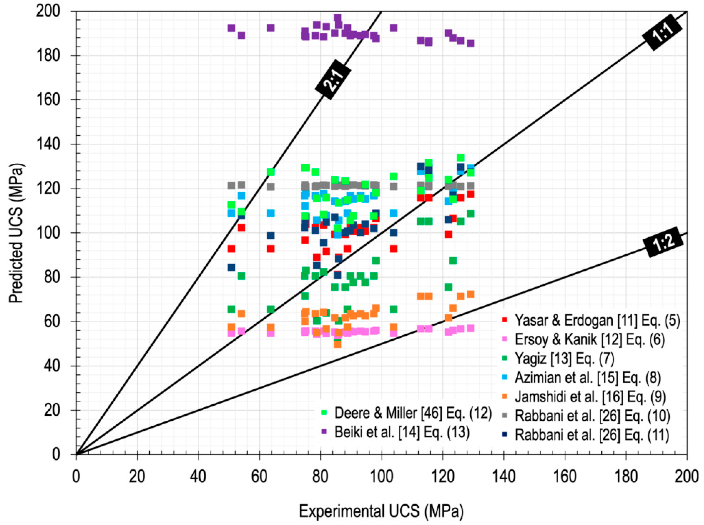
3.1. UCS Prediction from Selected Bibliography

As indicated by González et al. [18], the existing simple correlations for limestone from the literature were not suitable for the ‘Antofagasta’ limestone, which implied the development of a multiple correlation in which more variables (v_p, ρ_sat and n) were introduced to increase the fit of the experimental equation, and to be able to characterize the rock with easily measurable properties. This is due to the fact that the UCS depends both on the index properties (v_p, ρ_dry, n, I_s(50), R_N, etc.), and on the petrofrabrics and internal pore distribution, as can be seen in the values of

Table 2. Existing simple and multiple analytical models between UCS (MPa) and index properties like v_p (km·s⁻¹), ρ_dry (g·cm⁻³) and n (%) for travertine and carbonate rocks.

Analytical Model	R2	Rock Type	Phase	Reference	Equation
${\mathrm{v}}_{\mathrm{p}}=0.0317\mathrm{UCS}+2.0195$	0.80	Carbonate rocks	Dry *	[11]	(5)
$\mathrm{UCS}=15\ln \left(1000{\mathrm{v}}_{\mathrm{p}}\right)-73$	0.86	Travertine	Dry *	[12]	(6)
$\mathrm{UCS}=0.26{\mathrm{v}}_{\mathrm{p}}^{3.453}$	0.85	Travertine, limestone and schist	Dry *	[13]	(7)
$\mathrm{UCS}=0.026{\mathrm{v}}_{\mathrm{p}}-20.207$	0.90	Marly rocks	Dry *	[15]	(8)
$\mathrm{UCS}=101.1\ln \left(1000{\mathrm{v}}_{\mathrm{p}}\right)-802.81$	0.945	Travertine	Dry *	[16]	(9)
$\mathrm{UCS}=143.8{\mathrm{e}}^{-0.0695\mathrm{n}}$	-	Carbonates and limestones (5 < n < 20%) (30 < UCS < 150 MPa)	Dry *	[26]	(10)
$\mathrm{UCS}=135.9{\mathrm{e}}^{-0.048\mathrm{n}}$	-	Carbonates and limestones (0 < n < 20%) (10 < UCS < 300 MPa)	Dry *	[26]	(11)
$\mathrm{UCS}=0.1984{\rho }_{dry}-362.7$	-	Basalt, diabase, dolomite, gneiss, granite, limestone, marble, quartzite, rock salt, sandstone, schist, siltstone and tuff	Dry	[45]	(12)
$\mathrm{UCS}=\frac{1.83}{\mathrm{n}}+\frac{0.07}{\mathsf{\rho }}+\frac{307}{{\mathrm{v}}_{\mathrm{p}}}+130$	0.54	Carbonate rocks	Dry *	[14]	(13)

* The authors do not explicitly indicate saturated or dry conditions, so it is assumed as dry (S_r = 0).

. Likewise, the UCS depends on the size of the specimen [1,42], as well as the v_p [43,44], parameters that must be considered for the scale effect, when applying it to an engineering project.

In the case of travertine, the same occurs.

Table 3. Average obtained UCS values in strength tests and average predicted UCS values, as well as their relative errors according to different authors.

Equation	Predicted UCS (MPa)		Relative Error (%)
	Mean	SD	Mean	SD
(5)	101.085	9.044	–9.562	16.650
(6)	55.394	0.823	–65.301	35.301
(7)	79.360	15.094	16.950	23.426
(8)	115.620	7.454	–20.993	15.015
(9)	62.564	5.549	46.153	27.091
(10)	121.152	0.322	–24.291	16.889
(11)	105.265	13.277	–13.101	14.506
(12)	118.498	8.768	–22.607	15.952
(13)	189.695	2.726	–51.561	11.208

shows the different linear correlations that relate UCS with v_p, (Equations (5)–(9)), with n (Equations (10) and (11)) and ρ_dry (Equation (12)). Equation (13) corresponds to the multiple correlation that includes the three properties. Figure 2 shows how no correlation fits the experimental results (line 1:1), and Table 3 shows the mean values and relative errors. From these average values, it can be concluded that Equations (5) and (11) are the closest to 101.09 and 105.27 MPa, respectively (they have the lowest relative errors in absolute value). It should be noted that in the determination of these equations no travertine specimens were considered, only limestone, marble, dolomitic limestone, dolomite, marble and graveled limestone.

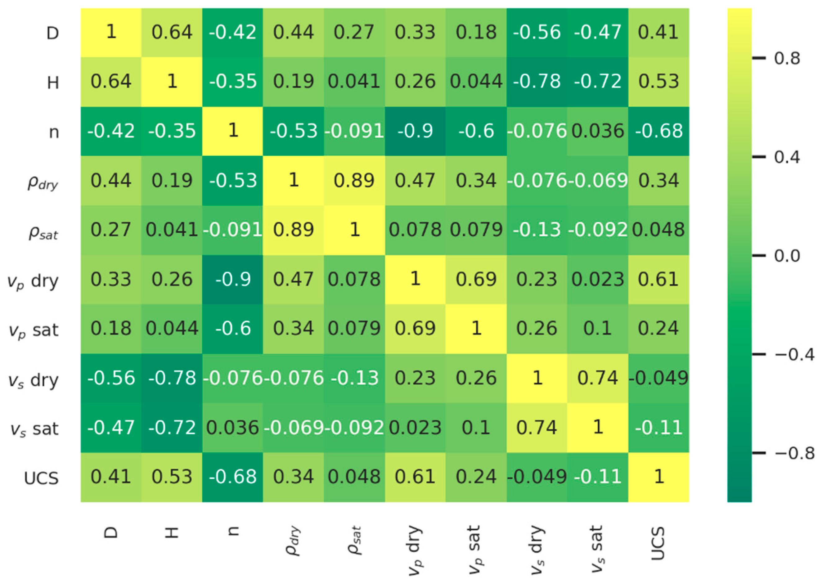
3.2. Correlation and Univariate Regression Analyses

Developing Pearson’s correlation analysis (Figure 3), the positive correlation between UCS and v_p,dry is highlighted, and the negative correlation between UCS and n. It is also observed that the UCS dependent variable does not have a strong linear correlation with the other sampled variables, especially with the ρ_sat, v_s,dry and v_s,sat variables, where there is no linear correlation (r = 0).

With the purpose of studying the relationship between the independent variables, v_p,dry (hereinafter referred to as v_p) and n, and the dependent variable (UCS), a simple regression model (Equations (14)–(19)) was set up, to model the compression strength as a function of the independent variable (considering the exponential and potential models, after log transformation). Additionally, the curvature is considered in the analytical model, to study its impact on the response variable (Equations (20) and (21)). The mathematical models generated as a function of v_p and n and the respective goodness-of-fit statistics (R²) are presented in

Table 4. Summary of univariant analytical models.

Fitting	Analytical Model	p-Value	R2 Statistic	Equation
Linear	$\mathrm{UCS}\left({\mathrm{v}}_{\mathrm{p}}\right)=-123.37+41.13{\mathrm{v}}_{\mathrm{p}}$	0.0000	0.6028	(14)
Linear	$\mathrm{UCS}\left(\mathrm{n}\right)=119.36-7.11\mathrm{n}$	0.0000	0.6788	(15)
Exponential	$\mathrm{UCS}\left({\mathrm{v}}_{\mathrm{p}}\right)=9.1369{\mathrm{e}}^{0.4379{\mathrm{v}}_{\mathrm{p}}}$	0.0000	0.6324	(16)
Exponential	$\mathrm{UCS}\left(\mathrm{n}\right)=120.6763{\mathrm{e}}^{-0.0749\mathrm{n}}$	0.0000	0.7114	(17)
Potential	$\mathrm{UCS}\left({\mathrm{v}}_{\mathrm{p}}\right)=2.2544{\mathrm{v}}_{\mathrm{p}}^{2.2325}$	0.0000	0.6167	(18)
Potential	$\mathrm{UCS}\left(\mathrm{n}\right)=115.32{\mathrm{n}}^{-0.2116}$	0.0000	0.7223	(19)
Quadratic	$\mathrm{UCS}\left({\mathrm{v}}_{\mathrm{p}}\right)=843.45-333.25{\mathrm{v}}_{\mathrm{p}}+36.11{\mathrm{v}}_{\mathrm{p}}^2$	0.0000	0.6804	(20)
Quadratic	$\mathrm{UCS}\left(\mathrm{n}\right)=130.81-14.69\mathrm{n}+0.96{\mathrm{n}}^2$	0.0000	0.7573	(21)

.

From the analysis of the observed data distributions in Figure 4, and considering the goodness-of-fit statistics presented in Table 4, the best model to explain the UCS as a function of v_p is the quadratic model (R² = 0.6804), while the model as a function of n that presents a better fit also is the quadratic model (R² = 0.7573). On the other hand, although the adjusted models presented in Table 4 yielded considerably high coefficients of determination, these equations only include one independent variable. Therefore, an analysis that considers a greater number of independent variables that affect the response variable jointly, and that help explain the variability of the response variable has the potential to improve the percentage of variability explained by the analytical model.

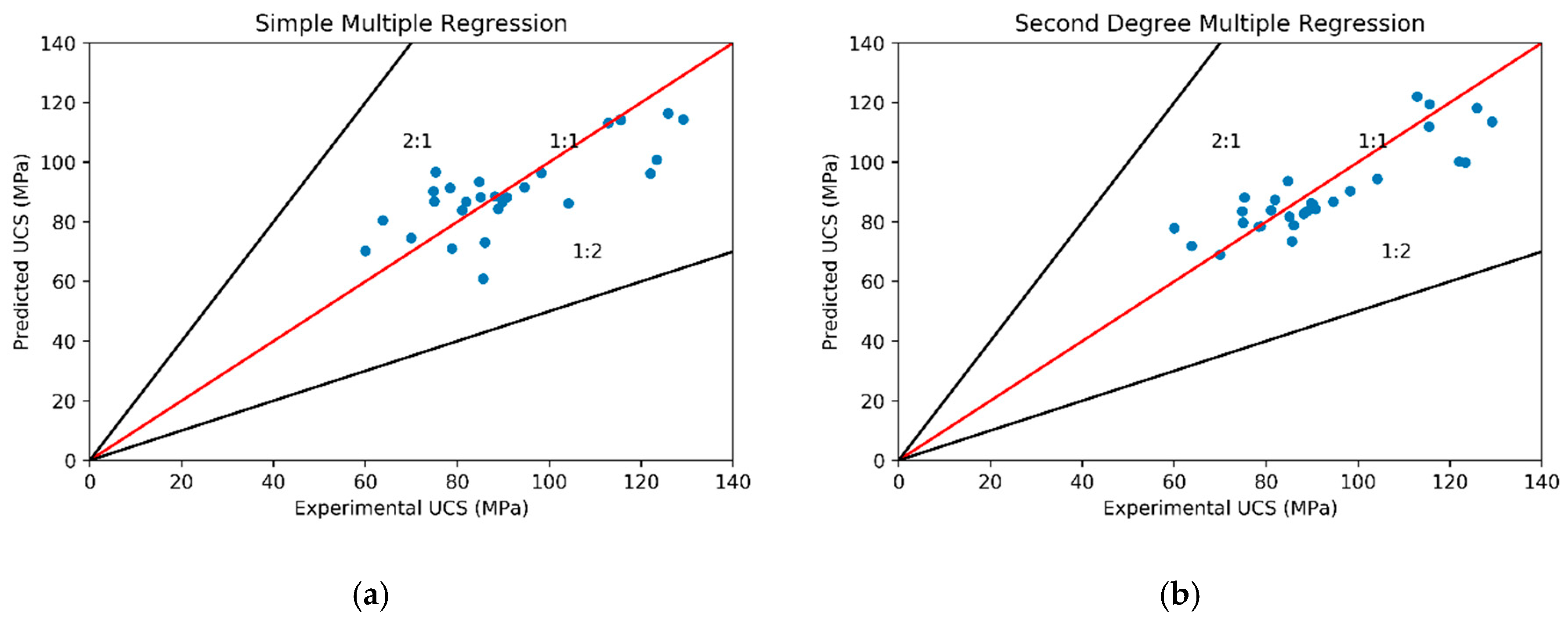
3.3. Multivariate Regression Analyses

By developing the multiple regression fitting and based on the information obtained from the ANOVA analysis, the first- and second-degree multiple regression models (Equations (22) and (23), respectively), shown in

Table 5. Summary of the multivariate analytical model.

Type of Fitting	Analytical Model	Var.	p-Value	F-Value	R2	Equation
Single multiple	${\mathsf{\sigma }}_{\mathrm{c}}\left({\mathrm{v}}_{\mathrm{p}},{\mathsf{\rho }}_{\mathrm{dry}},\mathrm{n}\right)=119.3575-7.1138\mathrm{n}$ (idem Equation (15))	Model	0.000	57.06	0.6788	(22)
		n	0.000	57.06
Quadratic multiple	$\begin{array}{ll}{\mathsf{\sigma }}_{\mathrm{c}}\left({\mathrm{v}}_{\mathrm{p}},{\mathsf{\rho }}_{\mathrm{dry}},\mathrm{n}\right)=-& 13648+2407{\mathrm{v}}_{\mathrm{p}}\\ & +5623{\mathsf{\rho }}_{\mathrm{dry}}+322\mathrm{n}\\ & -982{\mathrm{v}}_{\mathrm{p}}{\mathsf{\rho }}_{\mathrm{dry}}-10{\mathrm{v}}_{\mathrm{p}}\mathrm{n}\\ & -115{\mathsf{\rho }}_{\mathrm{dry}}\mathrm{n}\end{array}$	Model	0.000	20.01	0.8447	(23)
		${\mathrm{v}}_{\mathrm{p}}$	0.003	11.58
		${\mathsf{\rho }}_{\mathrm{dry}}$	0.003	11.09
		n	0.008	8.66
		${\mathrm{v}}_{\mathrm{p}},{\mathsf{\rho }}_{\mathrm{dry}}$	0.003	11.18
		${\mathrm{v}}_{\mathrm{p}},\mathrm{n}$	0.009	8.11
		${\mathsf{\rho }}_{\mathrm{dry}},\mathrm{n}$	0.023	5.99

, are able to represent the model in question for the set of sampled values. In addition, the linear effects and interactions of all factors must contribute greatly to explaining the experimental model.

The ANOVA test of the model indicates that the model presented in Equation (22) is adequate to represent the UCS under the range of established parameters, and although there is no lack of fit of the model, and the value of R² (0.6788) validates it (v_p and ρ_dry do not an effect in the response for the single multiple model), the effect of the other variables does not exceed the fit of the univariate models shown in Equations (18) and (20). Additionally, the p-value of Equation (22) indicates that the model is statistically significant.

On the other hand, the ANOVA test of the second degree model (Equation (23)) indicates that the model is also adequate to represent the response variable as a function of the independent variables, and the goodness-of-fit indicator R² (0.8447) validates this. The predicted and experimental UCS values are compared in Figure 5, where it is shown that the graphs of observed vs. predicted data generally follow the 1:1-line and the p value of the normality test of residuals are greater than the level of significance (value p > 0.05), indicating a good fit of the models presented in the Table 5.

3.4. Fitting of Artificial Neural Networks

With the aim of studying the fitting of the UCS by using models based on ANN’s, different architectures were generated, and their fitting was studied using the indicators of goodness of fit indicated above. Three artificial neural networks architectures were considered for training and testing, with network architectures of 1-2, 1-3 and 1-4 hidden layer and neurons per hidden layer, respectively. The statistics of the percentage of relative errors between the predicted responses and the measured values have been summarized in

Table 6. Goodness-of-fit statistics for artificial neural network (ANN) architectures.

Architecture/Statistic (Layer, Neurons)	Training				Testing
	MAD	MSE	ACC (%)	R2	MAD	MSE	ACC (%)	R2
1 layer, 2 neurons	0.0712	0.0469	85.00	0.6975	0.0856	0.0536	77.77	0.6646
1 layer, 3 neurons	0.0816	0.0523	85.00	0.6732	0.0975	0.0618	77.77	0.6371
1 layer, 4 neurons	0.0902	0.0587	85.00	0.6271	0.1012	0.0729	66.67	0.5582

.

From the analysis of the goodness-of-fit statistics of the different ANN configurations presented in Table 6, it can be checked that the model presenting the best fit in is the simplest configuration (one hidden layer with two neurons), which is validated by the highest determination coefficient (0.6975), a high accuracy (85%) and low errors (MAD and MSE). The increase of the coefficient of determination through the training and testing periods is presented in Figure 6.

3.5. Discussion

Table 7. Coefficients of determination of the generated models.

Model	Equation/Architecture	R2
Linear $\left[{\mathsf{\sigma }}_{\mathrm{c}}\left({\mathrm{v}}_{\mathrm{p}}\right)\right]$	(14)	0.6028
Linear $\left[{\mathsf{\sigma }}_{\mathrm{c}}\left(\mathrm{n}\right)\right]$	(15)	0.6788
Exponential $\left[{\mathsf{\sigma }}_{\mathrm{c}}\left({\mathrm{v}}_{\mathrm{p}}\right)\right]$	(16)	0.6324
Exponential $\left[{\mathsf{\sigma }}_{\mathrm{c}}\left(\mathrm{n}\right)\right]$	(17)	0.7114
Potential $\left[{\mathsf{\sigma }}_{\mathrm{c}}\left({\mathrm{v}}_{\mathrm{p}}\right)\right]$	(18)	0.6167
Potential $\left[{\mathsf{\sigma }}_{\mathrm{c}}\left(\mathrm{n}\right)\right]$	(19)	0.7223
Quadratic $\left[{\mathsf{\sigma }}_{\mathrm{c}}\left({\mathrm{v}}_{\mathrm{p}}\right)\right]$	(10)	0.6804
Quadratic $\left[{\mathsf{\sigma }}_{\mathrm{c}}\left(\mathrm{n}\right)\right]$	(21)	0.7573
Multiple simple $\left[{\mathsf{\sigma }}_{\mathrm{c}}\left({\mathrm{v}}_{\mathrm{p}},{\mathsf{\rho }}_{\mathrm{dry}},\mathrm{n}\right)\right]$	(22)	0.6788
Multiple quadratic $\left[{\mathsf{\sigma }}_{\mathrm{c}}\left({\mathrm{v}}_{\mathrm{p}},{\mathsf{\rho }}_{\mathrm{dry}},\mathrm{n}\right)\right]$	(23)	0.8447
ANN $\left[{\mathsf{\sigma }}_{\mathrm{c}}\left({\mathrm{v}}_{\mathrm{p}},{\mathsf{\rho }}_{\mathrm{dry}},\mathrm{n}\right)\right]$	(1 layer, 2 neurons)	0.6975

presents the results of both the regression analyses and the best ANN architecture. Regression models and their fit are presented, relating UCS (dependent variable) first with v_p or n (linear, exponential, potential and quadratic models) and then including all rock parameters for the travertine stone studied (multiple regression and neural network models). Simple regression analyses found that UCS is related to v_p and n, and the best fit was obtained with a quadratic model (R² = 0. 7573), dependent only on the porosity of the rock, while the neural network model is the one that presents the best fit for multivariate modeling, considering the totality of adjusted models.

Neural network analyses are competitive with single and multiple linear regression analyses, but not with the quadratic multiple model (model that presents the best fit). However, due to the lack of sample data, the adjustment potential of the tool and its ability to abstract the modeled system is not evident.

4. Conclusions and Future Works

The combined effect of v_p, ρ_dry and n in UCS for travertine-saturated cylindrical specimens was studied. It is evident that v_p and n have a synergistic effect in UCS (both individually and combined), while ρ_dry does not have a statistically significant influence (linear, exponential, potential, and quadratic) on the dependent variable. This is explained by the fact that, for the same rock type, the density remains relatively constant, since the measured porosity only affects the external pores of the test specimen, which do not necessarily have to be interconnected with the internal ones. Therefore, v_p may vary, but density does not, and, therefore, there is no correlation between them.

The experimental results were analyzed through simple regression analysis (or in its absence, after log transformation) to develop the analytical models that best adapt to UCS depending on v_p (as developed by most authors). Subsequently, multiple regression analysis and an artificial neural network model (ANN) were performed, to obtain a predictive model of UCS from v_p, n and ρ_dry.

Simple regression analyses (using only v_p or n as independent variable) showed a better R² value of 0.7573 for the univariate model, dependent only on porosity, while the univariate model dependent on v_p turned out to be the quadratic adjustment, with an R² of 0.6804. On the other hand, a multiple regression analysis, considering interactions between factors and quadratic terms resulted in a better R² value (0.8447), which indicates a better adjustment when additional explanatory variables are considered. Multiple regression analyses were also able to identify ρ_dry as a statistically non-significant independent variable for predicting UCS from ultrasonic pulse transmission tests. Finally, the ANN-based model presented a competitive fit with the single and multiple linear regression models in predicting UCS (R² = 0.6975), showing that UCS is directly dependent on the independent variables v_p, ρ_dry and n.

To continue this research line with travertine, the incorporation of a greater number of independent variables in the analysis and a larger number of samples is planned. This research aims to identify the variables that explain the experimental variability of UCS under sampling conditions, and to model the dynamics of the system using machine learning algorithms, such as neural networks or Bayesian networks [46]. The possible variables to be considered are the corrected point load index (I_s(50)), and the number of Schmidt’s hammer rebounds (R_N). Further tests will be carried out to try to improve the analytical models.

References

1. Hoek, E.; Brown, E.T. Underground Excavations in Rock; Institution of Mining and Metallurgy: London, UK, 1980. [Google Scholar]
2. Barton, N.; Lien, R.; Lunde, J. Engineering classification of rock masses for the design of tunnel support. Rock Mech. 1974, 6, 189–236. [Google Scholar] [CrossRef]
3. Bieniawski, Z.T. Engineering Rock Mass Classifications; Wiley: Rotterdam, The Netherlands, 1989. [Google Scholar]
4. Romana, M. A geomechanical classification for slopes: Slope Mass Rating. In Comprehensive Rock Engineering; Hudson, J.A., Ed.; Pergamon: London, UK, 1993; Volume 3, pp. 575–600. [Google Scholar]
5. ISRM. The Complete ISRM Suggested Methods for Rock Characterization, Testing and Monitoring: 1974−2006. In Commission on Testing Methods, International Society for Rock Mechanics; Ulusay, R., Hudson, J.A., Eds.; ISRM Turkish National Group: Ankara, Turkey, 2007. [Google Scholar]
6. ISRM. The ISRM Suggested Methods for Rock Characterization, Testing and Monitoring: 2007−2014. In Commission on Testing Methods, International Society for Rock Mechanics; Ulusay, R., Ed.; Springer: Dordrecht, The Netherlands, 2015. [Google Scholar]
7. ASTM D5873-14. Standard Test Methods for Determination of Rock Hardness by Rebound Hammer Method; American Society for Testing and Materials: Conshohocken, PA, USA, 2014. [Google Scholar]
8. ASTM D5731-16. Standard Test Methods for Determination of the Point Load Strength Index of Rock and Application to Rock Strength Classifications; American Society for Testing and Materials: Conshohocken, PA, USA, 2016. [Google Scholar]
9. ASTM D7012-14. Standard Test Methods for Compressive Strength and Elastic Moduli of Intact Rock Core Specimens under Varying States of Stress and Temperatures; American Society for Testing and Materials: Conshohocken, PA, USA, 2017. [Google Scholar]
10. ASTM D4543-19. Standard Test Methods for Preparing Rock Core as Cylindrical Test Specimens and Verifying Conformance to Dimensional and Shape Tolerances; American Society for Testing and Materials: Conshohocken, PA, USA, 2019. [Google Scholar]
11. Yasar, E.; Erdogan, Y. Correlating sound velocity with the density, compressive strength and young’s modulus of carbonate rocks. Int. J. Rock Mech. Min. Sci. 2004, 41, 871–875. [Google Scholar] [CrossRef]
12. Ersoy, H.; Danik, D. Multicriteria decision-making analysis based methodology for predicting carbonate rocks’ uniaxial compressive strength. Earth Sci. Res. J. 2012, 16, 65–74. [Google Scholar]
13. Yagiz, S. P-wave velocity test for assessment of geotechnical properties of some rock materials. Bull. Mater. Sci. 2011, 34, 947–953. [Google Scholar] [CrossRef]
14. Beiki, M.; Majdi, A.; Givshad, A.D. Application of genetic programming to predict the uniaxial compressive strength and elastic modulus of carbonate rocks. Int. J. Rock Mech. Min. Sci. 2013, 63, 159–169. [Google Scholar] [CrossRef]
15. Azimian, A.; Ajalloeian, R.; Fatehi, L. An Empirical Correlation of Uniaxial Compressive Strength with P-wave Velocity and Point Load Strength Index on Marly Rocks Using Statistical Method. Geotech. Geol. Eng. 2014, 32, 205–214. [Google Scholar] [CrossRef]
16. Jamshidi, A.; Nikudel, M.R.; Khamehchiyan, M.; Sahamieh, R.Z.; Abdi, Y. A correlation between P-wave velocity and Schmidt hardness with mechanical properties of travertine building stones. Arab. J. Geosci. 2016, 9, 568. [Google Scholar] [CrossRef]
17. Goodman, R.E. Introduction to Rock Mechanics, 2nd ed.; Wiley: New York, NY, USA, 1989. [Google Scholar]
18. González, J.; Saldaña, M.; Arzúa, J. Analytical Model for Predicting the UCS from P-Wave Velocity, Density, and Porosity on Saturated Limestone. Appl. Sci. 2019, 9, 5265. [Google Scholar] [CrossRef] [Green Version]
19. ASTM 122-17. Standard Test for Calculating Sample Size to Estimate, with Specified Precision, the Average for a Characteristic of a Lot or Process; American Society for Testing and Materials: Conshohocken, PA, USA, 2019. [Google Scholar]
20. IAEG. Classification of rocks and soils for engineering geological mapping part I: Rock and soil materials. Bull. Int. Assoc. Eng. Geol. 1979, 19, 364–371. [Google Scholar]
21. Palchik, V.; Hatzor, Y.H. Crack damage stress as a composite function of porosity and elastic matrix stiffness in dolomites and limestones. Eng. Geol. 2002, 63, 233–245. [Google Scholar] [CrossRef]
22. Palchik, V.; Hatzor, Y.H. Influence of porosity on tensile and compressive strength of porous chalks. Rock Mech. Rock Eng. 2004, 37, 331–341. [Google Scholar] [CrossRef]
23. Zhang, Q.; Song, J. The Application of Machine Learning to Rock Mechanics. In Proceedings of the 7th ISRM Congress, Amsterdam, The Netherlands, 16–20 September 1991; pp. 833–837. [Google Scholar]
24. Yilmaz, I.; Yuksek, G. Prediction of the strength and elasticity modulus of gypsum using multiple regression, ANN, and ANFIS models. Int. J. Rock Mech. Min. Sci. 2009, 46, 803–810. [Google Scholar] [CrossRef]
25. Dehghan, S.; Sattari, G.H.; Chelgani, S.C.; Aliabadi, M.A. Prediction of uniaxial compressive strength and modulus of elasticity for Travertine samples using regression and artificial neural networks. Min. Sci. Tech. 2010, 20, 41–46. [Google Scholar] [CrossRef]
26. Rabbani, E.; Sharif, F.; KoolivandSalooki, M.; Moradzadeh, A. Application of neural network technique for prediction of uniaxial compressive strength using reservoir formation properties. Int. J. Rock Mech. Min. Sci. 2012, 56, 100–111. [Google Scholar] [CrossRef]
27. Barzegar, R.; Sattarpour, M.; Nikudel, M.R.; Moghaddam, A.A. Comparative evaluation of artificial intelligence models for prediction of uniaxial compressive strength of travertine rocks, Case study- Azarshahr area, NW Iran. Model. Earth Syst. Environ. 2016, 2, 76. [Google Scholar] [CrossRef] [Green Version]
28. Ching, J.; Phoon, K.; Li, K.; Weng, M. Multivariate Probability Distribution for Some Intact Rock Properties. Can. Geotech. J. 2019, 18, 1–18. [Google Scholar] [CrossRef] [Green Version]
29. May, G.; Hartley, A.J.; Chong, G.; Stuart, F.; Turner, P.; Kape, S.J. Eocene to Pleistocene lithostratigraphy, chronostratigraphy and tectono-sedimentary evolution of the Calama Basin, northern Chile. Chil. Geol. J. 2005, 32, 33–58. [Google Scholar] [CrossRef]
30. Bezerra, M.A.; Santelli, R.E.; Oliveira, E.P.; Villar, L.S.; Escaleira, L.A. Response surface methodology (RSM) as a tool for optimization in analytical chemistry. Talanta 2008, 76, 965–977. [Google Scholar] [CrossRef]
31. Dean, A.; Voss, D.; Draguljić, D. Design and Analysis of Experiments, 2nd ed.; Springer: Cham, Germany, 2017. [Google Scholar]
32. Berger, P.D.; Maurer, R.E.; Celli, G.B. Experimental Design, 2nd ed.; Springer: Cham, Germany, 2018. [Google Scholar]
33. Montgomery, D.C. Design and Analysis of Experiments, 8th ed.; John Wiley & Sons: New York, NY, USA, 2012. [Google Scholar]
34. Walpole, R.; Myers, R.; Myers, S.; Ye, K. Probabilidad y Estadística para Ingeniería y Ciencias; Pearson: Ciudad de México, Mexico, 2012. [Google Scholar]
35. Haykin, S. Neural Networks and Learning Machines, 3rd ed.; Pearson: New York, NY, USA, 2008. [Google Scholar]
36. Wu, Y.C.; Feng, J.W. Development and Application of Artificial Neural Network. Wirel. Pers. Commun. 2018, 102, 1645–1656. [Google Scholar] [CrossRef]
37. Grosan, C.; Abraham, A. Intelligent Systems: A Modern Approach; Springer: Dordrecht, Germany, 2011. [Google Scholar]
38. Soete, J.; Kleipool, L.M.; Claes, H.; Claes, S.; Hamaekers, H.; Kele, S.; Özkul, M.; Foubert, A.; Reijmer, J.J.G.; Swennen, R. Acoustic properties in travertines and their relation to porosity and pore types. Mar. Petrol. Geol. 2015, 59, 320–335. [Google Scholar] [CrossRef] [Green Version]
39. Weger, R.J.; Eberli, G.P.; Baechle, G.T.; Massaferro, J.L.; Sun, Y.-F. Quantification of pore structure and its effect on sonic velocity and permeability in carbonates. AAPG Bull. 2009, 93, 1297–1317. [Google Scholar] [CrossRef]
40. Karakul, H.; Ulusay, R. Empirical Correlations for Predicting Strength Properties of Rocks from P-Wave Velocity under Different Degrees of Saturation. Rock Mech. Rock Eng. 2013, 46, 981–999. [Google Scholar] [CrossRef]
41. Schön, J.H. Physical properties of Rocks. In Handbook of Petroleum Exploration and Production; Elsevier: Amsterdam, The Netherlands, 2011. [Google Scholar]
42. Wang, S.; Masoumi, H.; Oh, J.; Zhang, S. Scale-Size and Structural Effects of Rock Materials; Woodhead Publishing: Duxford, UK, 2020. [Google Scholar]
43. Fener, M. The Effect of Rock Sample Dimension on the P-Wave Velocity. J. Nondestr. Eval. 2011, 30, 99–105. [Google Scholar] [CrossRef]
44. Ercikdi, B.; Karaman, K.; Cihangir, F.; Yilmaz, T.; Aliyazıcıoğlu, S.; Ayhan, K. Core size effect on the dry and saturated ultrasonic pulse velocity of limestone samples. Ultrasonics 2016, 72, 143–149. [Google Scholar] [CrossRef]
45. Deere, D.U.; Miller, R.P. Engineering Classification and Index Properties for Intact Rock; Technical Report No. AFWL-TR-65-116; Air Force Weapons Lab/Kirtland Air Force Base: Albuquerque, NM, USA, 1966. [Google Scholar]
46. Saldaña, M.; González, J.; Jeldres, R.; Villegas, Á.; Castillo, J.; Quezada, G.; Toro, N. A Stochastic Model Approach for Copper Heap Leaching through Bayesian Networks. Metals 2019, 9, 1198. [Google Scholar] [CrossRef] [Green Version]
Figure 1. Structure of an artificial neural network.
Applsci 10 04565 g001
Figure 2. Predicted vs. Experimental UCS values.
Applsci 10 04565 g002
Figure 3. Correlation plot of sampled variables.
Applsci 10 04565 g003
Figure 4. Relationship between UCS and independent variables: P-wave velocity and porosity for analytical models (a,b) linear, (c,d) exponential, (e,f) potential and (g,h) quadratic.
Applsci 10 04565 g004
Figure 5. Predicted UCS vs. experimentally determined UCS for simple multiple regression (a) (Equation (22)) and second degree multiple regression (b) (Equation (23)).
Applsci 10 04565 g005
Figure 6. Variation of the coefficient of determination R2 vs. epochs for neural network architecture of 1 hidden layer, 2 neurons.
Applsci 10 04565 g006