Text Normalization Using Encoder–Decoder Networks Based on the Causal Feature Extractor

Abstract

The encoder–decoder architecture is a well-established, effective and widely used approach in many tasks of natural language processing (NLP), among other domains. It consists of two closely-collaborating components: An encoder that transforms the input into an intermediate form, and a decoder producing the output. This paper proposes a new method for the encoder, named Causal Feature Extractor (CFE), based on three main ideas: Causal convolutions, dilatations and bidirectionality. We apply this method to text normalization, which is a ubiquitous problem that appears as the first step of many text-to-speech (TTS) systems. Given a text with symbols, the problem consists in writing the text exactly as it should be read by the TTS system. We make use of an attention-based encoder–decoder architecture using a fine-grained character-level approach rather than the usual word-level one. The proposed CFE is compared to other common encoders, such as convolutional neural networks (CNN) and long-short term memories (LSTM). Experimental results show the feasibility of CFE, achieving better results in terms of accuracy, number of parameters, convergence time, and use of an attention mechanism based on attention matrices. The obtained accuracy ranges from 83.5% to 96.8% correctly normalized sentences, depending on the dataset. Moreover, the proposed method is generic and can be applied to different types of input such as text, audio and images.

1. Introduction

Research in natural language processing (NLP) has traditionally focused on the resolution of problems such as automatic bilingual translation [1], text summarization [2], automatic text generation [3] and text classification [4]. However, there are also other not so well-known problems that are often overlooked, despite being as difficult to solve as the former ones. In particular, the problem of text normalization is one such case. Its definition is simple: Given an arbitrary text, transform it into its normalized form. This normalized form depends on the context in which we are working. For example, in the context of text-to-speech (TTS) systems—which is the objective of this paper—normalizing a text means rewriting it as it should be read, for example:

$$\begin{array}{cc}\hfill \mathit{I}\mathit{have}\$20& \to \mathit{I}\mathit{have}\mathit{twenty}\mathit{dollars}\hfill \\ \hfill \mathit{It}\mathit{happened}\mathit{in}1984& \to \mathit{It}\mathit{happened}\mathit{in}\mathit{nineteen}\mathit{eighty}\mathit{four}\hfill \\ \hfill \mathit{He}\mathit{weights}\mathit{50}\mathrm{kg}& \to \mathit{He}\mathit{weights}\mathit{fifty}\mathit{kilograms}\hfill \end{array}$$

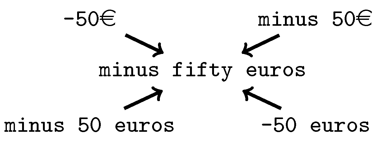
At first glance, this problem might seem trivial and rather unimportant. Nevertheless, text normalization is a ubiquitous task, present in most NLP problems. The reason is that normalizing the input as a first step significantly decreases the complexity of those subsequent tasks, since equivalent phrases—yet differently written—end up being exactly the same phrase, as illustrated in Figure 1. WaveNet [5] is an example of these systems, where a generative model for TTS is trained with normalized text as input.

Despite its apparent simplicity, this problem entails an interesting challenge. Data-driven approaches, specifically Deep Learning, deserve special attention since: (1) There exists a general belief that Deep Learning can solve any problem; and (2) it is the framework used in this research. Text normalization gathers three main features that make it challenging for this type of techniques, as it has been already discussed by Sproat and Jaitly [6]. In short:

• Non-trivial cases (i.e., those whose output and input differ) are sparse.
• It is context-dependent, for example, a normalized date could change depending on the local variant of the language.
• There is no natural reason for building a text normalization database. Everyone knows that 2 means two.

Different models have been developed to tackle this problem. The first attempts date back to the times when researchers were developing the first complete TTS systems, as described by Sproat and Jaitly [6]. Systems based on traditional techniques include finite state automata as well as finite state transducers [7]. The usage of these models has the advantage of being well-known techniques that work (and fail) as expected; yet, these solutions need to be hand-crafted from scratch for each language, suffering from lack of flexibility (which translates into an increase in production costs).

Nowadays, many researchers are moving towards Deep Learning models, that try to learn how to solve the problems from the data itself [6]. However, the amount of information that these models require to work correctly can be prohibitive. In the cases where the target language is low-resourced, that is, a language for which little data is available, rule-based solutions have been attempted [8], as well as Deep Learning models that make use of data augmentation techniques to compensate the lack of samples [9]. In particular, this system is based on an encoder–decoder architecture, using bidirectional recurrent neural networks working at character-level; this is similar to our proposed approach, except for the encoder and other adjustments of the network.

Text normalization is also a very common step in the analysis of social media messages, where the input text is prone to present problems of misspelling, abbreviation, incorrect grammar, etc. For example, Arora and Kansal [10] proposed a system to perform sentiment analysis in Twitter messages using Convolutional Neural Networks (CNN), with text normalization as a preprocessing step. Their method is based on character-level embedding (instead of the most common word-level embedding), with convolutional, max-pooling and fully connected layers, achieving a classification accuracy above 98.1%. However, the normalization step is based on traditional techniques using tokenization, dictionary word replacement, lemmarization and stemming.

The models proposed by Sproat and Jaitly [6] deserve special attention. They are based on Deep Learning techniques and, at each time-step, they read a character and produce an entire word, thus being character-based at the input, and word-based at the output. These models obtained a high accuracy performance (one case achieving a 99.8% on the English test set). Unfortunately, they suffered from the so-called silly, undetectable or unrecoverable errors. This means that these errors cannot be detected only looking at the produced output. For example, this is the case when normalizing I’m 12 as I am thirteen, yet the error Im twenty could be detected in the subsequent process. Our hypothesis is that these errors could be due to the use of recurrent word-level models, and they could be avoided to a large extent by a character-level approach. More recently, this model was improved in [11], by using a covering grammar for the given language, with the purpose of avoiding those unrecoverable errors. This grammar constrains the execution of the recurrent neural network, with the particularity that these grammars can be learned automatically from the samples.

The present approach has been designed with two main goals in mind. The first one is offering a solution for the text normalization problem that exclusively uses neural networks, taking advantage of the benefits of data-driven solutions. The second goal is to introduce convolutional components in the neural model, substituting its recurrent counterparts and, thus, speeding up the whole process. Moreover, proving the usefulness of such convolutional architecture would help to push even further the idea that CNNs can be used outside of a computer vision framework.

The main contributions of this work are as follows: (1) Proposal of a character-based approach for the text normalization problem which does not suffer from undetectable or unrecoverable errors; (2) introduction of a new general-purpose encoder based on causal convolutions, the Causal Feature Extractor (CFE); and (3) a variation of the traditional attention mechanisms, in which a context matrix is generated, instead of a context vector.

2. Materials and Methods

2.1. Text Normalization Dataset

As stated in Section 1, it can be challenging to obtain a valid database of normalized text. Fortunately, a huge database was built and released to the whole Machine Learning community by Sproat and Jaitly [6]. This dataset occupies a total of 9.1 Gb and contains about 40 million phrases extracted from Wikipedia. It includes 1.1 billion words of English text. The expected output for the input sentences was mostly obtained with a set of hand-built rules used by a finite-state grammar [12].

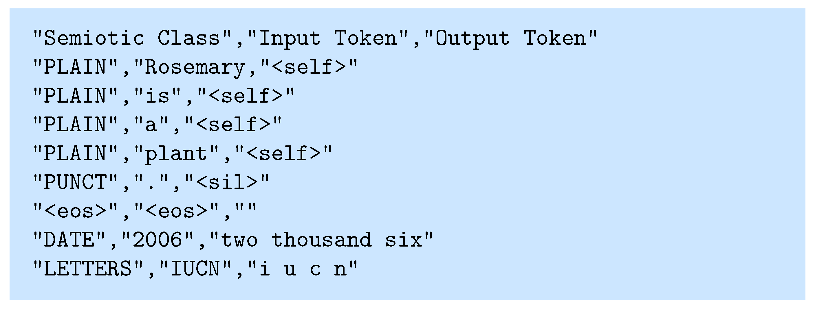
The database was prepared for their word-level model and, therefore, requires some preprocessing before being suitable for a character-level approach. Particularly, each entry on the original database is a pair of words (or special symbols) plus an additional column describing its semiotic class, as shown in Figure 2. In order to use a character-level approach, each row needs to be composed of all the words belonging to the same phrase, and information regarding each individual word (such as its semiotic class) has to be disregarded.

As shown in Figure 2, there are special symbols in the original dataset, namely: (1) <eos>, denoting the end of the current sentence; (2) <sil>, marking a silence (comma, colon, and so on); and (3) <self>, meaning that the output in that entry is the same as the input. Since these symbols cannot be used in a character-level approach (due to the alignment problem), they were removed in the following way: <eos> disappears once the sentence has been recomposed; whereas <sil> and <self> are substituted by the corresponding input.

Other minor changes have been made on the original dataset to speed up the training process, obtaining a new dataset as shown in Figure 3. The process consists of the following steps:

• Concatenation of the words belonging to the same phrase and removal of special symbols, as mentioned before.
• Phrases with non-permitted characters are discarded, keeping an alphabet of $v=127$ characters, including numbers, basic arithmetic symbols, currency, and the English alphabet.
• Entries with an output longer than 177 characters are discarded as well, which corresponds to removing only 0.01% of the sentences.
• Entries are sorted in descending order with respect to their output length. This way, the padding introduced in batches is minimized and, as described by Xu et al. [13], convergence speed is increased without a significant loss in accuracy.

2.2. Character-Level Encoding

Regarding the actual input and output used in the model, we use a one-hot encoding, i.e., a string $s=s_1{s}_2\dots s_l$ of size $l\in \mathbb{N}$ is transformed into a matrix $\mathbf{X}\in {\mathbb{M}}_{v\times l}$, where the i-th column $x_i\in \mathbf{X}$ is set to zero in all positions except the one corresponding to the index of the character $s_i$, according to the model alphabet. Recall that v is the size of the alphabet (127 in our case).

The advantages and disadvantages of using a character-level model—as opposed to word-level models—have been described by some authors, since it appears as a basic design decision in many NLP problems. Four arguments in favor of character-level approaches are shown, three of them introduced by Chung et al. [14], and the last one given by Lee et al. [15]:

• Out-of-vocabulary issues do not appear, as it could happen in word-level models. We could suffer from out-of-alphabet issues, but these can be easily solved.
• Such approaches are able to model rare morphological variants of a word.
• Input segmentation is no longer required.
• By not segmenting into words, the models have to discover the internal rules and structure of the sentences by themselves.

Since text segmentation is known to be problematic and error-prone, even for well-known languages such as English, removing this step without losing performance is a significant advantage to consider. Moreover, we can provide an additional argument for character-level approaches: If the model uses attention mechanisms, observing the attention matrices after a particular sample gives a better understanding of the system’s logic and the language itself. For example, consider the case where the model transforms 2s into two seconds; its attention matrix could potentially show that the last letter was produced by looking at the number.

2.3. Encoder–Decoder Architecture

The encoder–decoder architecture is a common and popular design in recent Neural Machine Translation literature [16]. The model is composed of two parts: (1) An encoder that takes the input $\mathbf{X}$ (in this case, a phrase), and produces an intermediate representation $\mathbf{Z}$ (or code) that highlights its main features; and (2) a decoder that processes that set of features and produces the required output $\mathbf{Y}$ (in this case, a normalized phrase). $\mathbf{Z}$ is a matrix of size $\mathbf{Z}\in {\mathbb{M}}_{f\times l}$, where f represents the selected number of features to encode for each input value. 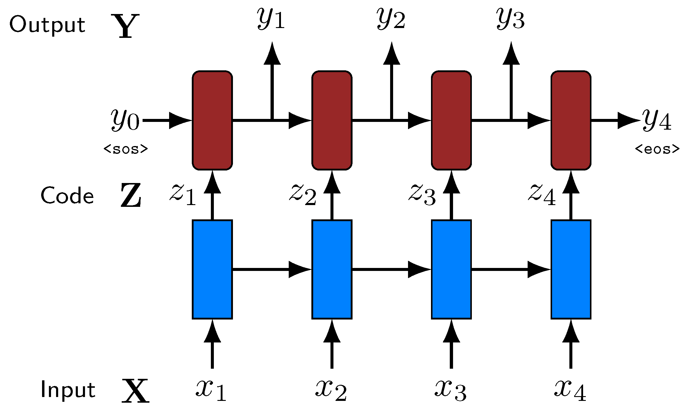Figure 4 shows a basic diagram of this model.

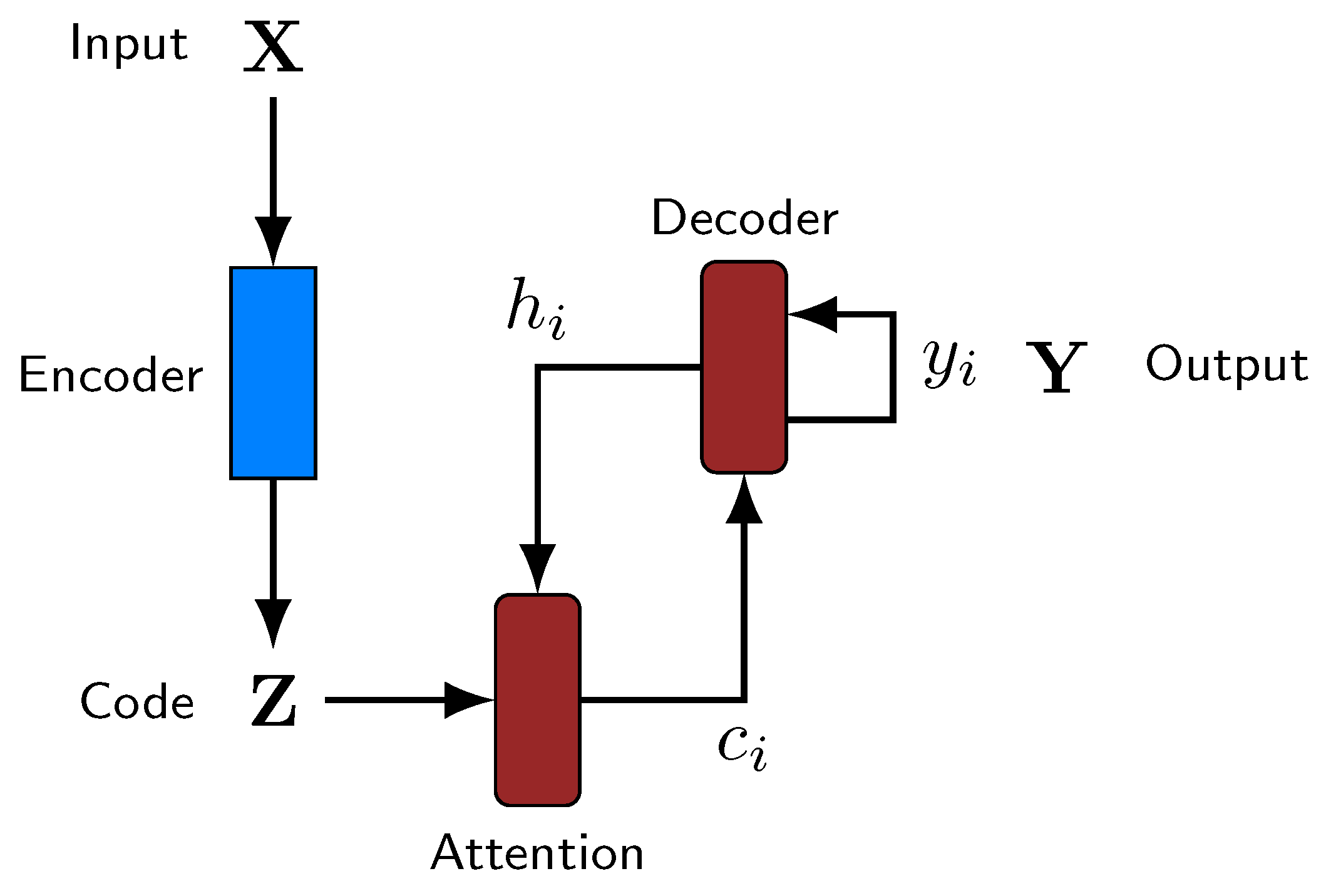
This is a simplified representation of the encoder–decoder architecture, involving that the size of the input, the intermediate representation and the output is the same. This can be the case, for example, of many image processing tasks. Nevertheless, in many NLP problems, they can have different sizes. In our case, the intermediate code always has the same length, l, as the input, but the length of the output can be different. The end of the output is determined by the production of an <eos> symbol. Thus, a more precise diagram of the model is presented in Figure 5.

There is a trend in using Long Short-Term Memory (LSTM) neural networks as encoders and decoders (for example, Sutskever et al. [17]) due to their ability to capture long dependencies among the elements of a sequence. Our proposed model uses an LSTM network as decoder. However, different encoders have been analyzed, including the proposed one, and their performances have been tested and compared.

Besides, some additional techniques that are common in the deep learning field were applied to improve the effectiveness of the system, such as batch processing (processing the input in batches of a certain size), dropout [18,19] (randomly removing some neurons with a given probability), weight normalization [20] (regularizing the weights of the neuronal layers), gradient clipping [21] (limiting the norm of the gradient), and decaying learning rate combined with the Adam optimizer [22] (progressively reducing the learning rate used in the backpropagation algorithm).

Attention Mechanisms

The basic encoder–decoder model is a very powerful and useful architecture, but some key issues arise when it is put into practice. Two of them stand out and are worth mentioning: (1) As shown in Figure 4, at each time step, the decoder only works with the code produced at that moment, hindering the usage of long-term dependencies; and (2) output and input need to have the same length, as previously mentioned, limiting its application to many practical problems.

We overcome these two restrictions by making use of attention mechanisms [23]. The idea behind them, depicted in Figure 5, is simple: First, produce the codes of the whole input sequence at once and, at each time step, let the decoder choose the most interesting elements of the input based on the latest output.

This can be expressed in mathematical terms as follows. Suppose that $\mathbf{Z}=z_1{z}_2\dots z_l$ is the obtained intermediate representation. The attention mechanism consists of a fully connected neural network with one hidden layer, taking as input $\mathbf{Z}$ and the vector $h_t$ of the hidden state of the LSTM decoder at each time step t. This network produces a vector of interesting features $a\in {\mathbb{M}}_{f\times 1}$. This vector a describes the characteristics that are expected to be obtained, so it is compared with each column of $\mathbf{Z}$, $z_i$, using the dot product as a function of similarity. So, a vector $\alpha \in {\mathbb{M}}_{1\times l}$ is generated in this way:

$$\alpha ={\alpha }_1{\alpha }_2\dots {\alpha }_l=(a·z_1,a·z_2\dots a·z_l)$$

(1)

Then, this vector $\alpha$ is transformed into a stochastic vector, i.e., a vector such that $\sum {\alpha }_i=1$, via:

$${\alpha }_i^{\prime }=\frac{exp{\alpha }_i}{{\sum }_{j}exp{\alpha }_j}$$

(2)

Now, ${\alpha }_i^{\prime }$ represents the interest of the decoder with respect to the i-th element of the code, $z_i$, at the given time step. With this information, a context vector is produced, that is, a vector representing the portion of the input that is actually interesting for the decoder at this instant. Traditionally, this context vector is given by a weighted sum of the elements of $z_i$, weighted by ${\alpha }^{\prime }$, i.e., $c={\sum }_i{\alpha }_i^{\prime }{z}_i$. Another possibility is to select only the code $z_i$ corresponding to the highest ${\alpha }_i^{\prime }$. However, we propose a different approach which consists in selecting several codes with the highest ${\alpha }_i^{\prime }$ values. Thus, instead of performing a weighted sum or taking the maximum, a new hyperparameter d is introduced to indicate the number of context elements that are considered. In this way, a context matrix $c\in {\mathbb{M}}_{f\times d}$ is generated at each time step t, where the i-th column, $c_i$, corresponds to the vector ${\alpha }_j^{\prime }{z}_j$, where ${\alpha }_j^{\prime }$ is the i-th largest value of ${\alpha }^{\prime }$. That is, $c_1$ corresponds to the largest value of ${\alpha }^{\prime }$, $c_2$ to the second largest value, etc. Subsequently, the decoder receives this context matrix, c, instead of just a context vector.

The idea inspiring this modification is that taking the average of the feature vectors involves a significant loss of information. Instead, by using the d greatest elements, the internal semantic of them is preserved.

2.4. Proposed Causal Feature Encoder

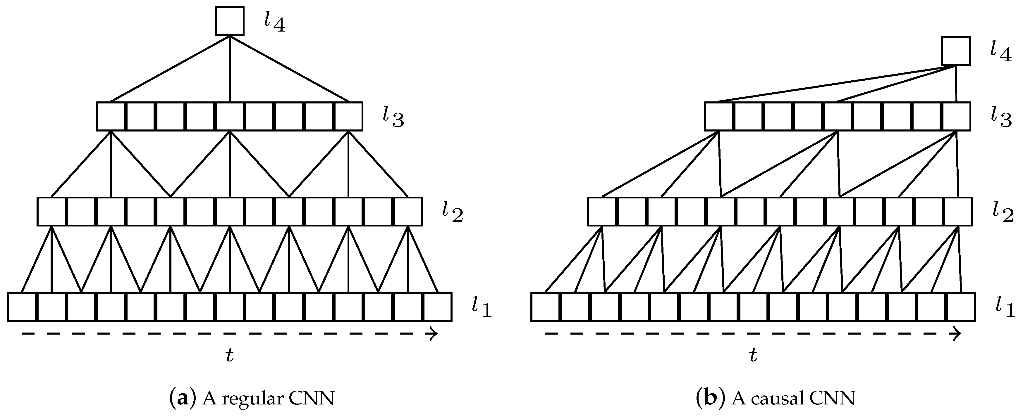
In this paper we propose a new type of encoder, the Causal Feature Extractor (CFE), that can be described as a two-step modification of a traditional CNN. The first change is that, instead of using regular convolutions, causal convolutions are applied; this concept was introduced by van den Oord et al. [5]. Figure 6a,b show a basic representation comparing a regular and causal neural network, respectively.

In a regular one-dimensional convolution, the output for a position t depends on the input values at $\dots t-2,t-1,t,t+1,t+2\dots$ Conversely, in a causal convolution, the output depends only on the inputs previous or posterior to that position, but never both. In other words, the causal convolution for t can use the values $t,t+1,t+2\dots$ or $t,t-1,t-2\dots$ This idea can be easily extended to images or, in general, to n-dimensional data.

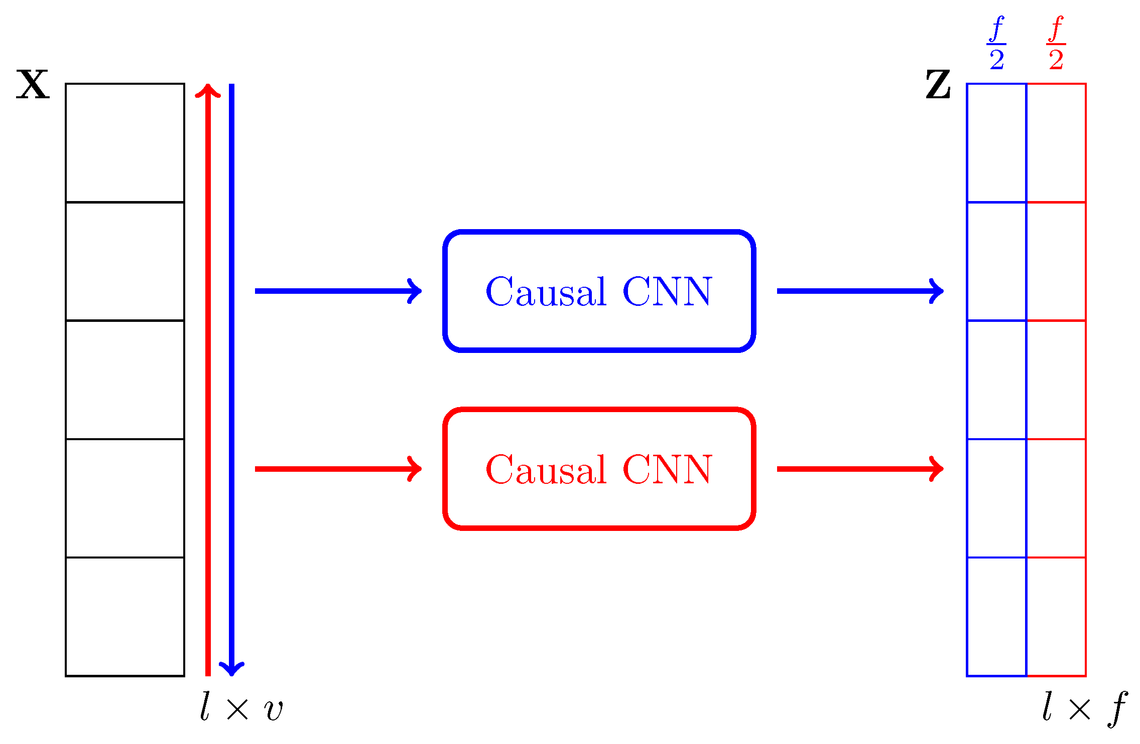
However, a convolution defined in such way only captures dependencies in one direction. To solve this important drawback, we propose a second change. To make the CFE bidirectional, in a similar fashion as it is done with LSTMs. Thereby, it contains two independent models that read the input in each direction, and their outputs are concatenated to produce the encoded representation. We depict this idea in Figure 7.

An additional technique is applied in the proposed encoder. Considering the long sequences that can be found in text normalization (in our datasets, up to 177 characters), we apply dilated convolutions to the convolutional models, as described by van den Oord et al. [5]. This technique consists in doubling the dilatation of each convolutional layer as it goes deeper into the structure, as depicted in Figure 6. So, in the first layer, the convolution for t depends on the input at $t,t-1,t-2\dots$; in the second layer, it depends on the previous layer at $t,t-2,t-4\dots$; in the third layer, $t,t-4,t-8\dots$, and so on. Moreover, the same for the opposite causal direction. By doing that, the actual receptive field of the model (i.e., the initial positions that contribute to the final result) is significantly increased without increasing the number of parameters of the network.

This new encoder has been designed to solve a problem that many applications of CNNs have with attention mechanisms. In previous experiments, it has been observed that CNNs tend to attend the wrong inputs according to our prior intuition. Namely, they choose the $i+C$-th element instead of the i-th element of the input, where C is a certain constant. Our intuition is that this could be caused by the padding introduced in each side of the input. By using causal convolutions, the model is forced to choose the outermost elements if it is interested in those.

2.5. Statistical Significance Test

When comparing the performance of various models, a critical aspect is to ensure that the obtained differences are statistically significant. It must be proved that those differences are significant, and not a mere product of the implicit variance of the training process. This is typically performed using some statistical test that asserts that the differences are actual differences up to some confidence level of probability, usually 95%.

In this paper, we have applied the approximate randomization test [24], also known as random permutation test. This statistical test measures the probability of the outputs of two different models of being indistinguishable, i.e., the probability that, by just looking at the predictions, we cannot tell whether they come from different models. The main reasons for using this method are: (1) It is computationally efficient; (2) it is distribution-free, meaning that it does not make any assumptions on the measured distribution; and (3) it is model-free, that is, the only required resources to perform the test are the actual predictions, making it suitable for any type of model.

Let us assume that the predictions of two different models are the ordered sets $A={\left\{a_i\right\}}_{i=1}^n$ and $B={\left\{b_i\right\}}_{i=1}^n$, and we have a function e that measures the similarity of the predictions with respect to the expected values, Y; for example, in our case e is the accuracy measure, defined as the percentage of correctly predicted characters with respect to the length of the output. Then, we can define the function:

$$t(A,B)=e(A,Y)-e(B,Y)$$

(3)

We want to estimate the probability of obtaining an error bigger than $t(A,B)$, assuming that both sets of predictions are indistinguishable, that is $P(X\ge t(A,B)H_0)$, where $H_0$ is the null hypothesis (i.e., both models are not significantly different).

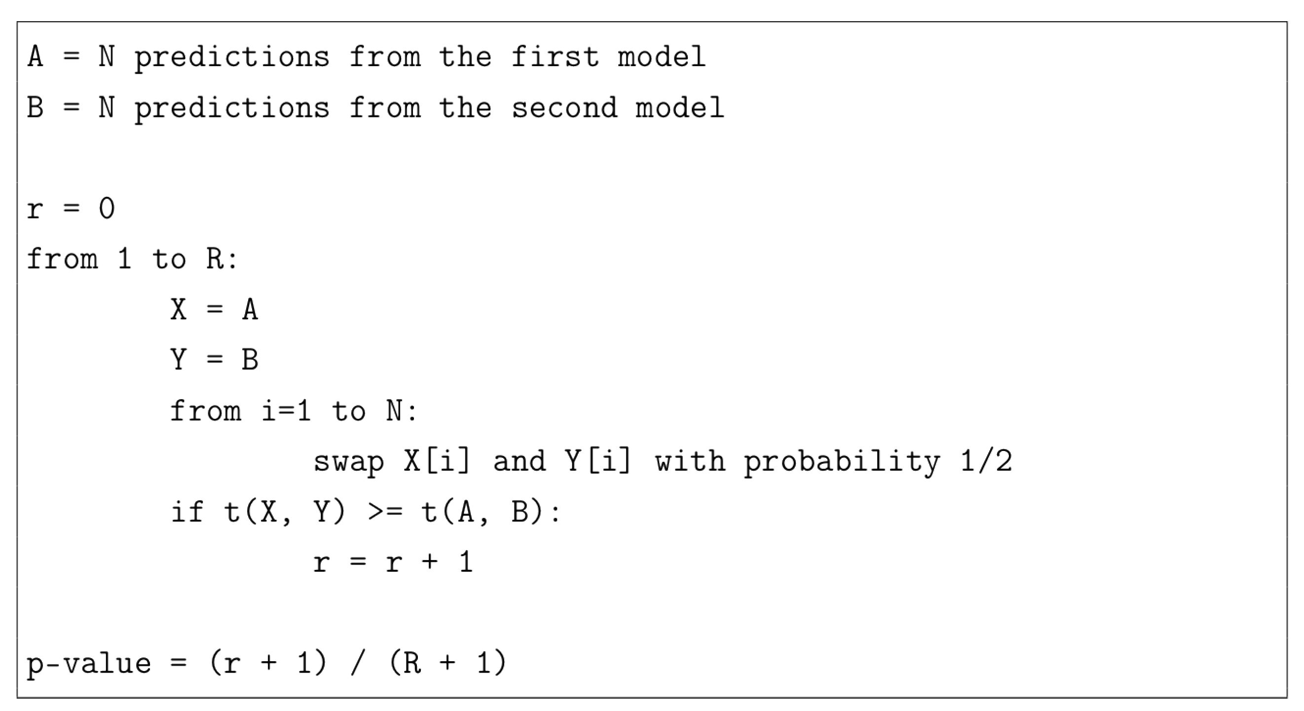
The algorithm to approximate this value consists in repeating many times the following process: Randomly swap each element of the first set with its counterpart in the second set; and count the number of times that the total error difference, measured by t, is greater or equal than the original one, that is, $t(A,B)$. Figure 8 shows the pseudocode of this algorithm. A small p-value, e.g., below 0.05, 0.02 or 0.01, indicates that the null hypothesis has to be rejected, so the models are significantly different.

In this test, the estimation of the p-value has an error itself, which is given by $\sqrt{p(1-p)/R}$, where p is the obtained p-value, and R is the number of iterations. If this error is too large, the p-value is unreliable; hence, the number of repetitions has to be computed to reduce the error [25]. In order to force the upper bound of the confidence interval of the estimated p being below the decision threshold, we need to find an R such that $l^2\alpha (1-\alpha )/P^2\le R$, where l is the confidence interval. Using P at $\alpha =0.05$ and requesting a 95% confidence interval, we get $R\ge 7600$. Consequently, that is the number of repetitions used in the tests.

3. Experimental Results

In the following subsections we describe the results obtained in this research, comparing the proposed encoder and other alternative methods. The last subsection is dedicated to the discussion of these results.

3.1. Experimental Setup

Three different experiments have been performed using different subsets of the filtered database, in order to analyze different aspects of the proposed model. The first two datasets are used to test and compare different models, whereas the latter is used to train the final model.

Table 1. Description of the datasets used in the experiments. Name: Dataset identifier. Duration: Time used for training the models. Training size: Number of samples used for training. Test/validation size: Number of samples used for test and for validation. Selection: Sample selection criteria.

Name	Duration	Training Size	Test/Validation Size	Selection
E1	1 h	50,000	10,000	shortest
E2	12 h	50,000	10,000	random
E3	22 h	1,000,000	200,000	random

shows their name, training time, number of training/test/validation samples, and how the samples were selected; random means that they were randomly taken, and shortest that the elements with shortest outputs were selected. In all the cases, the validation and test size is 1/5 of the training size, and all the sets are disjointed.

Training time is a key parameter in most deep learning systems, since it can determine the practical feasibility of a given method. Thus, accuracy is closely related with computational efficiency. For this reason, the comparison in the datasets is done by setting the duration of the training process, rather than fixing the number of training iterations or until reaching convergence.

For the execution of the experiments, all the computations were done in a remote server via secure shell and distributed between three NVIDIA GeForce GTX1080 GPUs (each experiment using a single GPU), in a computer with an i7-5930K Intel(R) CPU, 12 effective threads (6 with hyperthreading), and 600GB hard disk drive. Regarding the software, the code was mainly written in Python v.3.6, making use of the Pytorch v0.4 framework to build the neural models [26], as well as OpenNMT [27]. The latest is a neural machine translation toolkit used to speed up the process of solving and testing different problem solutions.

3.2. Proposed Methods and Number of Parameters

As stated before, the presented encoder–decoder architecture for text normalization was implemented in Python, using Pytorch and OpenNMT. In order to analyze whether the proposed CFE achieves a significant improvement, different existing encoders were taken into account. These alternative encoders (and their aliases) are the following:

LSTM

A 3 layer bidirectional LSTM network.

FCNN

A 4 layer fully CNN encoder, where the i-th element is an embedding of the i-th input, i.e., the encoded value only depends on the i-th input value.

FE

A traditional CNN with dilated convolutions. This is similar to the proposed CFE, but without considering causality.

CFE

The proposed Causal Feature Extractor encoder.

In all these cases, the only modification on the architecture resides in the the encoder. The decoder and attention mechanism remain always the same, that is, as they were described in the previous section. The hyperparameters of the models were manually tuned by trial and error, trying to obtain the best results. After that, the results presented here are averaged over five repetitions of the same models trained with different random seeds.

Table 2. Hyperparameters of the models used in the experiments.

Symbol	Description	Value
b	Batch size	128
f	Number of features produced by the encoder	256
s	Size of the internal hidden vectors of LSTM	128
d	Number of columns of the context matrix	10
$ml$	Number of neurons of the intermediate dense networks	256
w	Width of the convolutional filters	5
$rf$	Receptive field to be considered in the input	10
$lr$	Initial learning rate of Adam algorithm	0.001
$\beta$	Multiplier used in the decay of the learning rate	0.85
$step$	Number of iterations before applying the decay	400
$p_d$	Probability of disabling a neuron in the dropout	0.5
$p_t$	Probability of substituting a weight by expected value	0.4
$clip$	Upper limit of the norm of the gradient in the clipping	5

presents the selected hyperparameters.

The number of parameters of the four models used in the experiments are shown in

Table 3. Number of internal parameters of the models compared (in millions), considering only the encoder and the entire model (encoder + attention mechanism + decoder).

Number of Parameters of	LSTM	FCNN	FE	CFE
Encoder (millions)	1.102	0.285	0.111	0.111
Total (millions)	7.380	6.653	6.479	6.479

. These values correspond to the number of trainable parameters, i.e., the weights of the neural networks of each model, considering the encoder and the whole model. In general, the more parameters, the greater the complexity of the model is (and the greater the memory and time requirements are). So, for a similar performance, simpler models are usually preferred.

It can be observed that LSTM requires nearly 10 times more parameters than FE and CFE, while FCNN requires 2.5 times more parameters. This translates into a lower efficiency and speed of convergence of these models. In any case, the rest of the system (attention and decoder) has a considerably larger number of parameters, with about 6.3 million values that have to be trained. To initialize these parameters, the uniform method of Xavier [28] was used.

3.3. First Experiment

The purpose of this first experiment is to compare the accuracy achieved by the different methods in a reduced setup using the shortest entries containing: 50,000 training samples, 10,000 test samples, and 10,000 validation samples, as presented in Table 1. These values have been chosen so that the number of samples is large enough to train an accurate normalization model, but also small enough to require a reasonable training time that allows multiple repetitions. Specifically, training is limited to only 1 h in all cases. The obtained results are shown in

Table 4. Results obtained by the four models for the first experiment (E1). Encoder: Name of the encoder used. NLLLoss: Negative log-likelihood loss. CER: Character error rate. Acc (%): Accuracy. No. iters: Number of iterations. Rate: Iterations per second.

	Test			Validation
Encoder	NLLLoss	CER (%)	Acc (%)	No. Iters	Rate
LSTM	1.352	03.13	95.87	3620	1.005
FCNN	5.035	70.61	28.40	4370	1.214
FE	1.042	02.52	96.46	6980	1.939
CFE	0.952	02.24	96.83	6300	1.750

. Observe that these results are averaged over 5 runs and extracted from the test set, except from the results concerning the training speed, which are taken from the training logs. From left to right, the columns of Table 4 indicate the following parameters:

• Negative Log-Likelihood Loss (NLLLoss). It is the measure optimized by the neural networks during training, since it is the common measure used in classification problems.
• Character Error Rate (CER). It is defined as the mean Levenshtein distance [29] between the prediction and the expected value, that is, the minimum number of character insertions/deletions/substitutions required to change one sentence into the other, for all the test samples.
• Accuracy. It is a basic and well-known measure, defined as the percentage of correct output values, measured at a character level.
• Number of iterations performed during the training phase in the duration of the experiment (in this case 1 h).
• Rate. Number of iterations per second, on average, achieved during training.

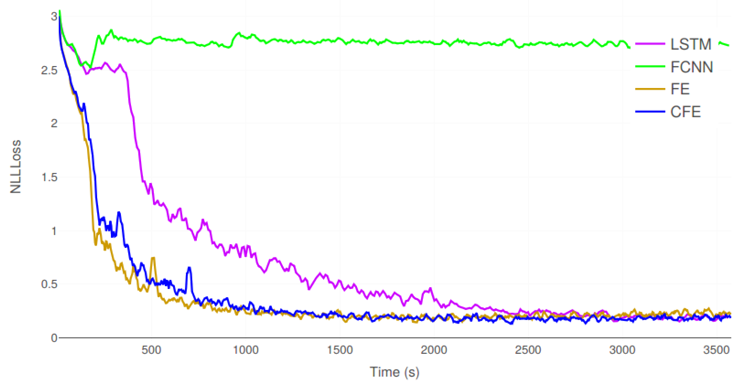
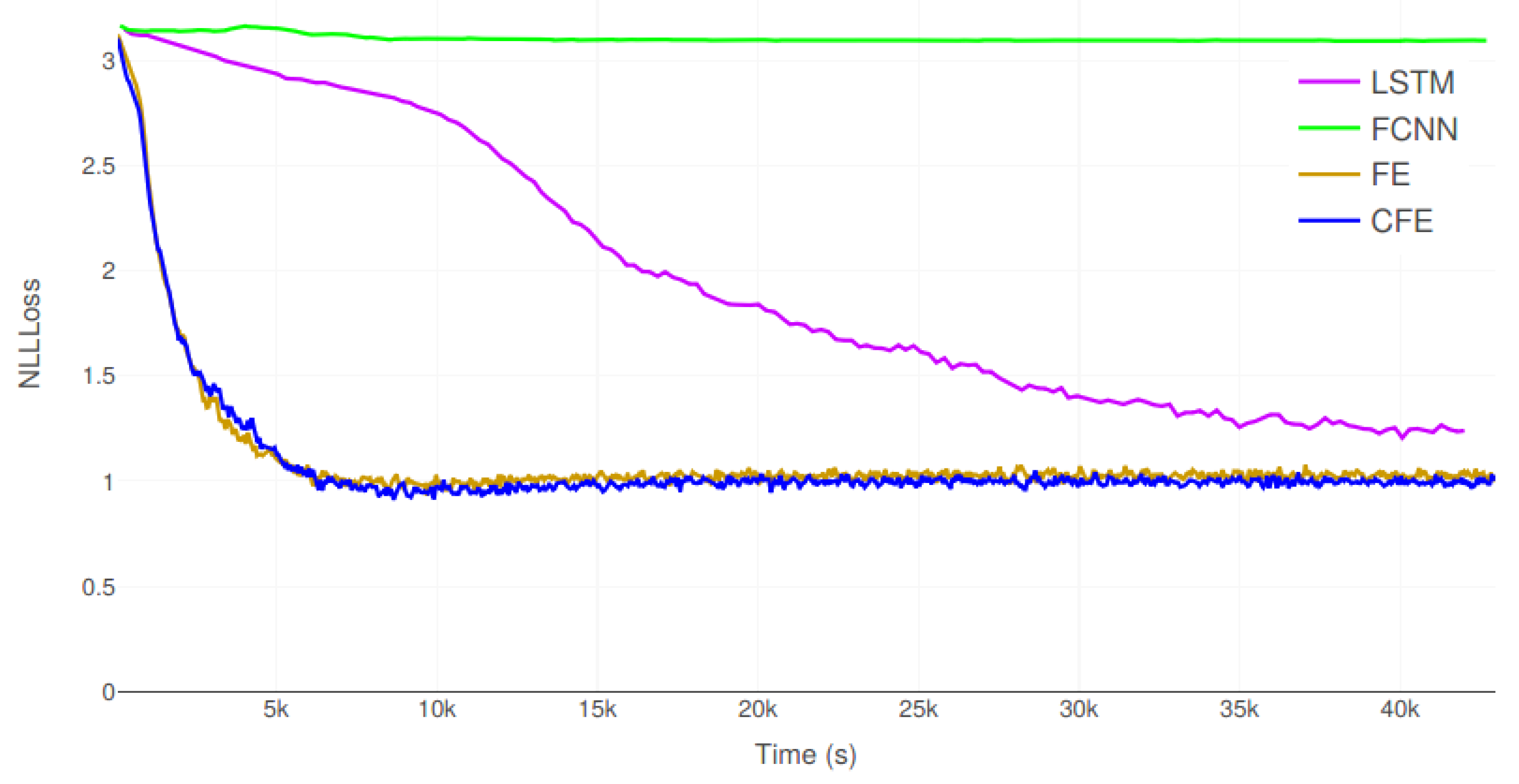
In order to get an in-depth view of the differences in the training process, Figure 9 shows the evolution of the NLLLoss of the validation samples for each model during training.

Table 5. p-Values of the first experiment (E1), indicating the probability of the null hypothesis, i.e., the probability that the results of the models are not distinguishable.

p-Value	LSTM	FCNN	FE	CFE
LSTM		0.0001	0.0001	0.0026
FCNN	0.0001		0.0001	0.0001
FE	0.0001	0.0001		0.0184
CFE	0.0026	0.0001	0.0184

shows the resulting p-values after running the approximate randomization test for each pair of models.

In this first experiment, CFE is clearly able to achieve the best results in terms of accuracy, CER and NLLLoss of the test set. It is interesting to observe that, although LSTM, FE and CFE tend to converge to the same NLLLoss values on the validation set, as shown in Figure 9, the differences are more prominent on the test set. Thus, the proposed method has a greater capacity for generalization on previously unobserved samples. Moreover, the statistical tests in Table 5 prove that these differences are significant. The probability that the results from FE and CFE are equivalent is below 2%. FCNN was unable to provide correct results, producing a very large character error rate. Concerning the computational efficiency, FE was able to execute almost 2 iterations per second. CFE is a 10% slower, but it is faster than the remaining methods.

3.4. Second Experiment

The objective of the second experiment is to compare the four encoders in a more complex scenario, where the samples were selected with more varied sizes. The number of samples of the training, test and validation datasets is the same as in the first experiment, but the samples are randomly selected from the whole dataset, with sizes varying at random between 1 and 177 characters (the maximum allowed length of the output, as justified in Section 2.1).

As before,

Table 6. Results obtained by the four models for the second experiment (E2). Encoder: Name of the encoder used. NLLLoss: Negative log-likelihood loss. CER: Character error rate. Acc (%): Accuracy. No. iters: Number of iterations. Rate: Iterations per second.

	Test			Validation
Encoder	NLLLoss	CER (%)	Acc (%)	No. Iters	Rate
LSTM	3.310	25.59	71.06	8900	0.206
FCNN	5.396	82.09	17.90	17750	0.411
FE	2.680	11.93	83.38	36650	0.848
CFE	2.686	12.69	83.45	36200	0.838

presents the accuracy measures obtained by the four encoders for the second experiment. Figure 10 and

Table 7. p-Values of the second experiment (E2), indicating the probability of the null hypothesis, i.e., the results of the models are not distinguishable.

p-Value	LSTM	FCNN	FE	CFE
LSTM		0.0001	0.0001	0.0001
FCNN	0.0001		0.0001	0.0001
FE	0.0001	0.0001		0.0003
CFE	0.0001	0.0001	0.0003

show the evolution of the validation error and the results of the statistical tests, respectively.

Again, FE and CFE are the two best encoders, being able to achieve an accuracy above 83.3%, while LSTM only obtains a 71%. Moreover, FCNN is unable to function properly, with a poor 17.9%. In fact, all the performance measures of FE and CFE are very close, and so are their computational efficiencies. However, the statistical test, which is performed on the accuracy parameter, proves that CFE is significantly better than FE; the probability that they are indistinguishable is only 0.03%. Overall, the obtained results indicate that this experiment is far more complex than E1, which had a best accuracy of 96.8%. Moreover, the training time in E2 is 12 h, while it was only 1 h for E1. Figure 10 suggests that LSTM would need even more time to reach convergence; it not only performs fewer iterations per second, but it requires more iterations to converge.

3.5. Third Experiment

Unlike the other experiments, the purpose of dataset E3 is not to compare the different encoders, but to train the final architecture of the proposed CFE method with a more complete and complex input, in order to compare the obtained results with other state-of-the-art works reported in the literature. Therefore, the training set contains 1 million samples, and the test and validation sets have 200,000 samples each.

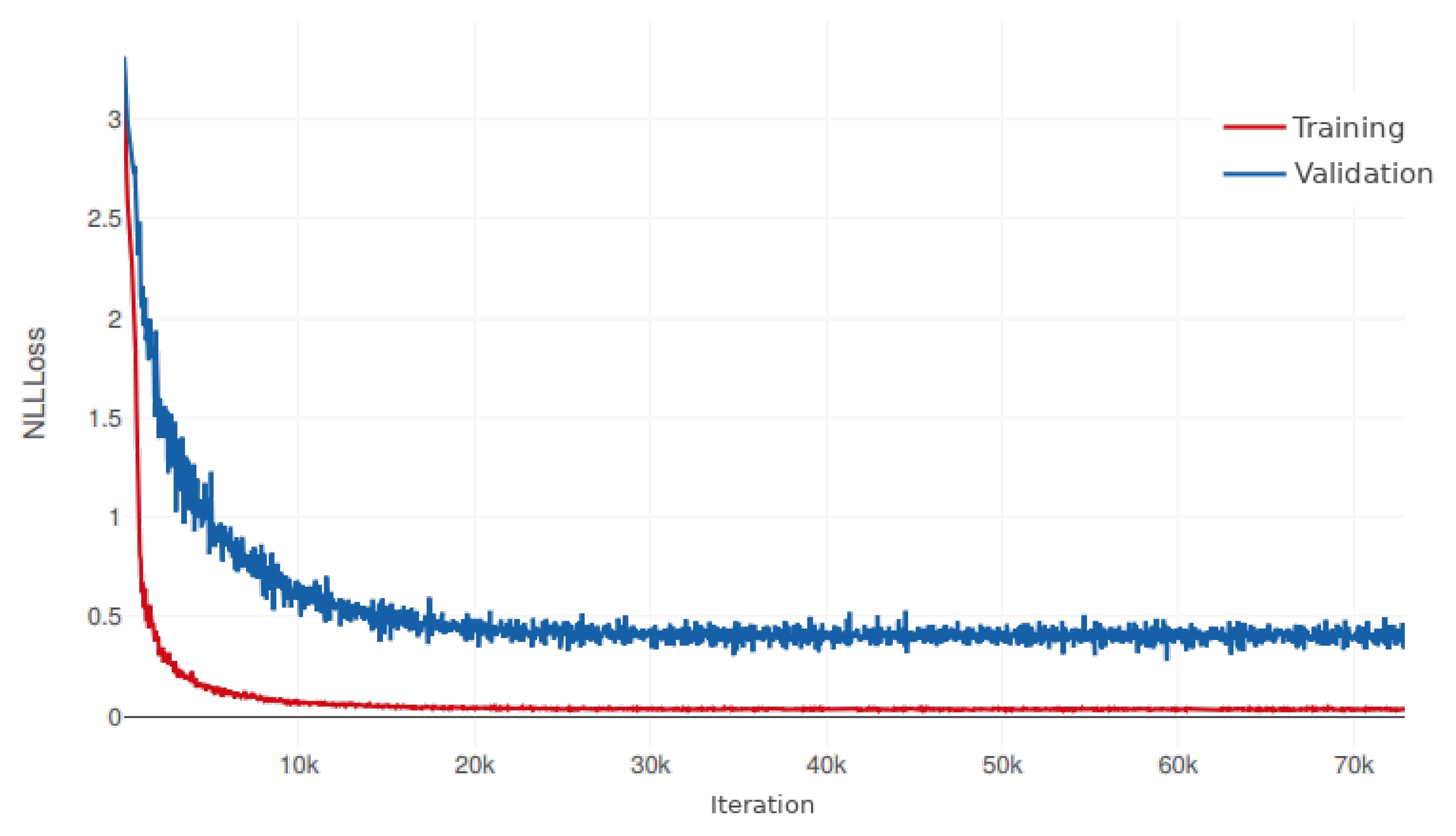
The architecture is identical to the one used in the previous experiments, with the hyperparameters presented in Table 2, and five repetitions. Figure 11 depicts the evolution of the training and validation errors during the training phase, and

Table 8. Results obtained by the proposed CFE encoder for the third experiment (E3). Encoder: Name of the encoder used. NLLLoss: Negative log-likelihood loss. CER: Character error rate. Acc (%): Accuracy.

	Test
Encoder	NLLLoss	CER (%)	Acc (%)
CFE	1.701	5.44	92.74

shows the accuracy measures obtained for the test set.

The accuracy measures achieved for E3 are between those obtained for E1 and E2, with a mean accuracy of 92.74% and a CER of 5.44. This indicates that although the test cases are more complex and varied than E2, having a larger training set is beneficial for the system. On the other hand, Figure 11 seems to indicate that convergence was reached long before the 22 h duration of the experiment.

3.6. Attention Matrices

In order to analyze whether the CFE encoder makes a better usage of the attention mechanisms than its non-causal counterpart, it is interesting to observe some actual examples and the attention matrices that they generate. These matrices are a representation of the decoder focus of interest while it was processing the input: The i-th row represents the i-th predicted character, and the j-th column is the model focus while predicting that character, i.e., the values of ${\alpha }_i^{\prime }$ (see Equation (2)).

The first case, shown in

Table 9. Predictions obtained by the four different models for a selected sample case in the experiment E1. The output produced by FCNN is incorrect since it falls in an infinite loop.

Input		23 Aug 2013.
Output		the twenty third of august twenty thirteen.
LSTM	✓	the twenty third of august twenty thirteen.
FCNN	✗	the twent t t eeeeeeeeeeeeeeeeeeeeee...
FE	✓	the twenty third of august twenty thirteen.
CFE	✓	the twenty third of august twenty thirteen.

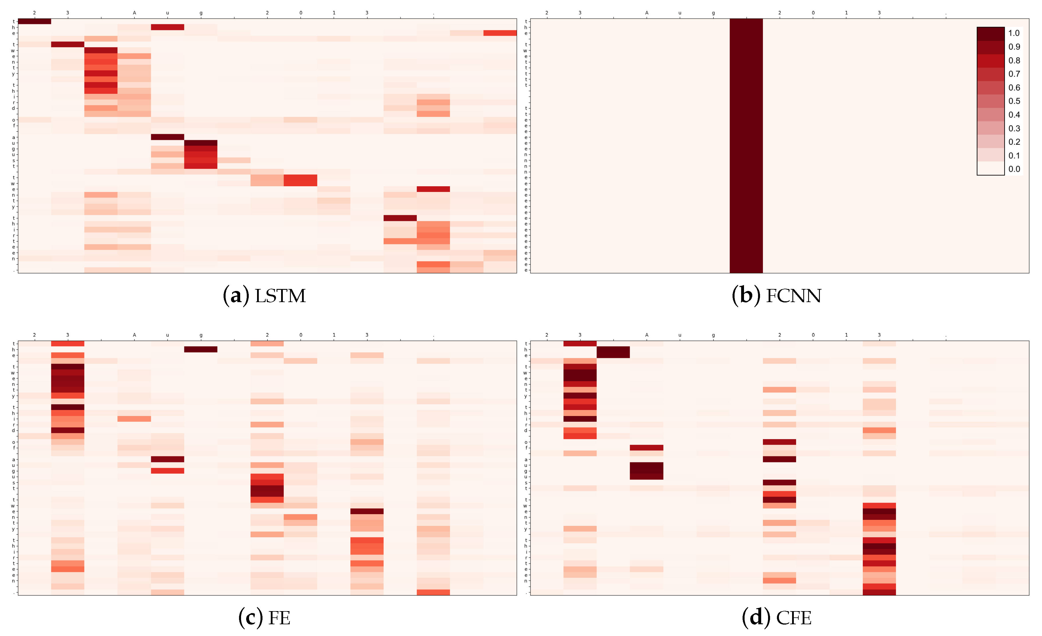
, is an example extracted from the test set of the first experiment, E1. The input phrase is “23 Aug 2013”. Regarding what would be ideally expected from the attention matrix, it should show three different phases: (1) First, it outputs the day while focusing on its digits; (2) then, the attention is moved towards the month; and (3) it finishes by looking at the year. Figure 12 shows the four attention matrices obtained.

The matrix obtained by CFE (Figure 12d) is the one that most closely resembles what one would expect from a useful attention mechanism. It clearly presents the three phases of this prediction, in which the system selects the day, the month and the year. FE and LSTM also follow this scheme, although not so clearly defined.

The second prediction selected to exemplify the use of the attention mechanism is taken from the test set of the second experiment, E2. It corresponds to the input sentence “Belpiela is a community in Tamale Metropolitan District in the Northern Region of Ghana.” This sample has been specifically selected because it is a longer case where the input and output are identical; thus, the ideally expected attention matrices should resemble an identity matrix.

Table 10. Predictions obtained by the four different models for a selected sample case in the experiment E2. Only the output obtained by CFE is correct.

Input		Belpiela is a community in Tamale Metropolitan District in the
		Northern Region of Ghana.
Output		Belpiela is a community in Tamale Metropolitan District in the
		Northern Region of Ghana.
LSTM	✗	Belpiela is a community in Tamale Metropolitan Disire
		egion te i e                         …
FCNN	✗	Th                              …
FE	✗	Belpiela is a community in Tamale Metropolitan District in the
		Northern Region Region of Ghana.
CFE	✓	Belpiela is a community in Tamale Metropolitan District in the
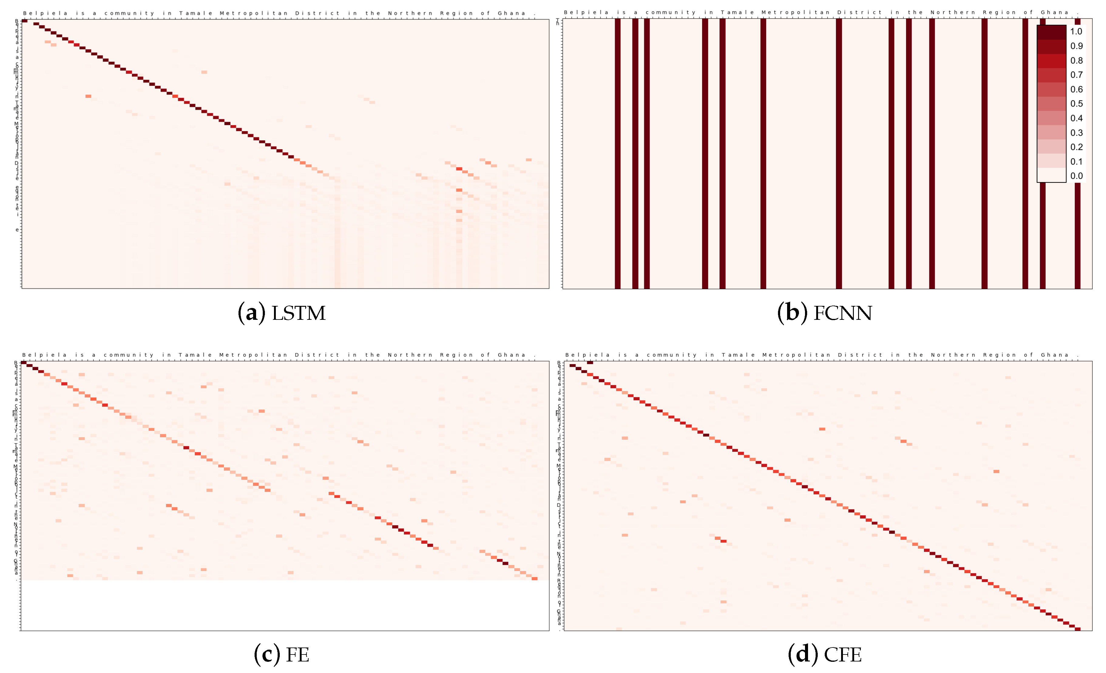
		Northern Region of Ghana.

shows the predictions obtained by the four models, whereas Figure 13 depicts the corresponding attention matrices.

Again, CFE is the only model that is able to produce a valid attention matrix, clearly resembling an identity. For this reason, it is the only method that was able to predict the correct output in this case. FE has a similar shape, but it produces some gaps which lead to a repetition of the word “Region” in the output.

3.7. Analysis of the Types of Errors

After analyzing the errors made by the proposed CFE method, we have observed that most of these errors can be classified into a reduced set of types. To get a better understanding of these types, all the incorrect predictions of CFE for the test set of the third experiment, E3, were dumped and classified by hand. Based on these observations, the taxonomy of error types has been defined as follows:

• T1. Infinite loop errors. The attention system of the model gets stuck and the maximum number of printed characters is reached. For example:

  Input

  Ruppert, Edward E.; Fox, Richard, S.; Barnes, Robert D. (2004).

  Output

  Ruppert, Edward e; Fox, Richard, s; Barnes, Robert d (two thousand four).

  Prediction

  Ruppert, Edward e; Fox, Richard, s R s , , , , , , , , , , , , , , , , , , , ...

• T2. Coincidental errors. Predictions where only a few isolated characters are wrongly printed. For example:

  Input

  The income was $11,091.

  Output

  The income was eleven thousand ninety one dollars.

  Prediction

  The income was fleven thousand ninety one dollars.

• T3. Early stop errors. Errors where the model finishes before processing the whole input. For example:

  Input

  Parmentier, Bruno (1 May 2000).

  Output

  Parmentier, Bruno (the first of may two thousand).

  Prediction

  Parmentier, Bruno (.

• T4. (Finite) jumps. The attention model finds the same pattern in the entry and repeats/oversees a part of it. For example:

  Input

  According to the 2011 census of India, Bhisenagar has 818 households.

  Output

  According to the twenty eleven census of India, Bhisenagar has eight hundred eighteen households.

  Prediction

  According to the twenty eleven census of India, Bhisenagar has eighteen households.

An automatic classification tool has been implemented in order to (approximately) quantify the errors according to their type. The results are shown in

Table 11. Distribution of the main types of errors made by the proposed CFE encoder for the test set of experiment E3.

Type	T1	T2	T3	Others	Total
Quantity	23,381	7159	50	10,696	41,286
Percentage (%)	56.63	17.34	0.12	25.9	100

where Others refers to the errors unclassified by the tool. Note that errors produced by jumps are not detected by the tool, since they can have different forms, but they represent a big portion of the unclassified errors.

As shown, more than half of the errors are produced by infinite loops. These are caused by a malfunction of the attention mechanism, that returns to a previously treated character. The same reason could be inferred for the errors of type T3, but these represent only a 0.12%. On the other hand, the errors of type T2 are most probably due to deficiencies in the decoder. Moreover, the category Others can be due to any component of the system.

Besides these types of errors, it is worth-mentioning that some observed errors were caused by the dataset itself, which contains some examples whose expected output is debatable (or simply incorrect). This was also observed by Sproat and Jaitly in [6], who estimated this error in a 0.1% of the total (although it was done in a manual analysis of only 1000 samples). These come from different sources, for example, from inconsistent rules for normalizing text among different entries, such as spelling or not spelling an acronym:

Input

Uppsala: Sprak och folkminnesinstitutet (SOFI).

Output

Uppsala: Sprak och folkminnesinstitutet (SOFI).

Prediction

Uppsala: Sprak och folkminnesinstitutet (S o f i).

Input

Chloroformic acid has the formula ClCO 2 H.

Output

Chloroformic acid has the formula c l c o two H.

Prediction

Chloroformic acid has the formula ClCO two H.

Or providing a few entries for rare cases that resemble too much to other more common cases:

Input

1980 A engine added to Transporter (T 3).

Output

one nine eight o A engine added to Transporter (T three).

Prediction

nineteen eighty A engine added to Transporter (T three).

Or inconsistencies in the entries (e.g., American vs British English):

Input

The mobilisation was announced by the mayor.

Output

The mobilization was announced by the mayor.

Prediction

The mobilisation was announced by the mayor.

Input

The Robinsons are a family in the soap opera Neighbours.

Output

The Robinsons are a family in the soap opera neighbors.

Prediction

The Robinsons are a family in the soapera Neighbors.

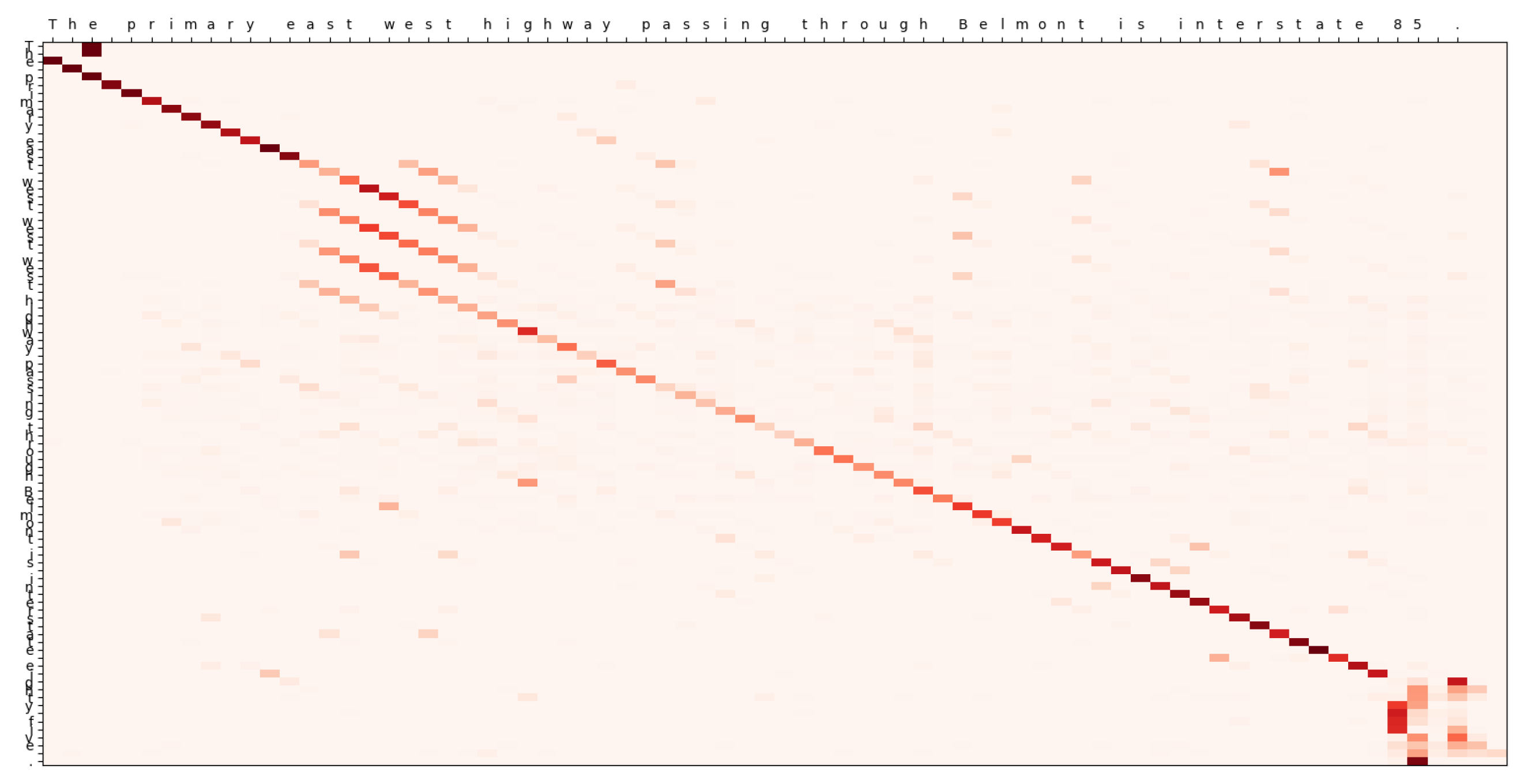
The proposed model also shows special difficulties deciding whether it should maintain capital letters on the predictions or not. This last sample also contains an example of overseeing parts of the input, probably because of the similarities between the words soap and opera. Another example of such jumps, in this case going backward in the input and thus repeating words, is the following:

Input

The primary east west highway passing through Belmont is interstate 85.

Output

The primary east west highway passing through Belmont is interstate eighty five.

Prediction

The primary east west west west highway passing through Belmont is interstate eighty five.

Which happened because the model confounds the suffix of west with the one of east as it can be seen on Figure 14. Attention matrices can be displayed for all these errors, shedding light on the underlying attention-related issues, except for the coincidental errors.

Finally, is it worth-noting the role of undetectable errors, since they were observed in previous works in the literature [6]. This type of error also appeared in the analyzed cases, as in the example shown for error type T4. However, in all the cases, they are a realization of another type of error that happens to be undetectable by chance, so the source of the error can be explained and solved. For example, the aforementioned error occurs as an occurrence of a jump error where the model confounds the first 8 with the third one of 818 when processing the input.

4. Discussion

This section discusses the results presented in Section 3. More specifically, the main questions raised in Section 1 can be formulated as follows:

• Can the problem of text normalization be solved solely by means of neural networks?
• Is such a solution viable using convolutional components? Which encoder is better?

Answering the first question, the most obvious result that we can extract based on any of the results from E1 and E2 (for example, Figure 10), is that the FCNN encoder does not work at all. Most probably, this erratic behavior comes from the differentiating feature of FCNN, that is, it extracts information from a single character of the input (instead of a neighborhood of it). This is a clear proof of an expected result: In order to work properly, the decoder cannot act on its own; extracting high level features from the surrounding characters is essential. So, the FCNN model should be discarded.

By looking at the second experiment, we can observe a significant difference between LSTM and its convolutional counterparts. Specifically, Table 6 shows that the accuracy of the convolutional encoders is about 12% higher than the LSTM encoder. Nevertheless, it could be the case that LSTM only needs more time to reach convergence. This leads us to the major differences between them: Number of parameters, convergence time, and iteration time. Three points strengthen this argument:

• Table 3 shows that the number of parameters of the LSTM encoder is ten times bigger than those of the convolutional encoders, making it harder to train and more expensive to use.
• Figure 9 and Figure 10 indicate that the LSTM encoder started to converge in E2 after 2 h 45 min of training, whereas the convolutional encoders were close to their minimum at 1 h 23 min.
• Regarding the iteration speed, Table 4 and Table 6 show that, besides being more accurate, the convolutional encoders operate around 2 and 4 times faster than the LSTM encoder, respectively.

This phenomenon can be explained by three reasons: (1) The aforementioned difference in the number of parameters; (2) the existence of recursive connections in LSTM, making it harder to optimize; and (3) the fact that convolutional networks run very fast on GPUs. Hence, this ensures that convolution-based encoders are viable, significantly faster, and statistically distinguishable from recurrent encoders (as proved by the tests in Table 7).

This solves the first part of question 2, whereas the second part concerns the selection of the best convolutional encoder. As show in Table 6, both encoders are quantitatively very similar, even though CFE obtains slightly better results and is distinguishable from FE. Qualitatively, CFE presents some advantages over FE regarding the attention mechanism:

• The first comparative of the attention matrices, Figure 12, shows that the three encoders behave in a similar fashion. However, CFE seems cleaner and more localized, since it knows better where to focus, distinguishing the three phases of this sample: Day, month, and year.
• The second comparative graphic, Figure 13, is even clearer. LSTM did not converge yet, so its prediction is far from the expected result. Regarding the convolutional encoders, CFE gets the example right, its attention matrix seems clean, and it resembles an identity matrix; whereas FE struggles to maintain the focus (many non-diagonal elements have taken attention) and makes erratic leaps (which results in missing words in the prediction, see Table 10).

Thus, it can be concluded that, in this case, CFE is preferable to FE due to its qualitative benefits and, to a lesser extent, its quantitative results. Regarding the undetectable errors reported in Sproat and Jaitly [6], it can be firmly confirmed that they are not an issue in these models as they appear by chance due to solvable errors. Specifically, these errors are highly related with the attention mechanism, as Table 11 shows, since the most common error is getting stuck in an infinite loop. These problems cause the model to lose focus and jump around when confounding similar parts of the input. Therefore, this could be greatly improved by using more sophisticated attention models that, for example, focus on local neighborhoods, take into account the index, or force the model to put more focus in the next character of the input.

Finally, we discuss the results obtained on the third experiment. Figure 11 shows that, during training, the model quickly converged. There is a gap between training and generalization error that the model has not been able to solve. However, the results obtained on the test set are very promising: It achieved 92.74% accuracy and 5.44% CER, against the 99.8% accuracy and 13.43% CER obtained by the models of Sproat and Jaitly [6] and Ikeda et al. [9], respectively. However, this comparison with previous works has to be carefully taken, since there are differences that do not allow a direct comparison. For example, in the case of [6], the dataset contains about 40 million sentences. This is translated into training times between 5 and 10 days using a system with eight GPUs. Compared to that, our method used 1 million sentences from the same dataset, and the training time was 22 h with 1 GPU. The difference is also in the underlying model of the encoder, which is a 4-layer bidirectional LSTM in [6] and the convolutional CFE encoder in our case, both working at character level. Lastly, in order to achieve the best accuracy of 99.8%, an additional finite state filter is applied to guide the decoding, while our method is exclusively based on neural networks.

Considering the second work, by Ikeda et al. [9], it must be noted that it is specific for Japanese text normalization. The system is also based on an encoder–decoder architecture, using bidirectional recurrent neural networks in the encoder, working at character-level. Nevertheless, the corpus is quite different, containing a set of over 200,000 synthesized sentences using 3500 Kanji characters; the training time was not reported.

Consequently, we consider that the results obtained by the proposed CFE are promising, and point out a viable direction to solve the problem of text normalization in a data-driven fashion. It is computationally less expensive than LSTMs, and the analysis of the errors has shown that it not prone to produce undetectable or unrecoverable errors, thus answering question 1.

5. Conclusions

In this paper, a new encoder–decoder architecture with attention mechanisms has been proposed for the problem of text normalization, using a character-level approach and introducing a new type of encoder. This encoder, called Causal Feature Extractor, is a novel technique designed to work properly in cooperation with the attention mechanisms. The experiments have empirically proven that this method is able to achieve very positive results, using the attention matrices more like it would be expected. Besides, it is able to work at least as good as the best of the compared encoders, and it brings all the benefits of using convolutional neural networks (e.g., computational efficiency and fast convergence). The last aspect that distinguishes this encoder from the traditional recurrent encoders is its simplicity to be adapted to other input layouts (for example, sound, images or video). Another contribution is the introduction of a new variation of the attention mechanisms, by using a context matrix instead of a vector.

Regarding previous works, the initial results have shown to be close to the state of the art, with much room for future improvements. Despite getting worse accuracy than the method presented in [6] (92.74% vs. 99.8%), it does not critically suffer from unrecoverable errors, nor it seems to concentrate its errors on any particular semiotic class, since most errors are attention-based; besides, the proposed method is less computationally expensive and does not include additional rule-based filters.

From a general point of view, an interesting result that can be extracted is the empirical proof that empowers the role of encoders in the encoder–decoder architectures. It has been shown that the system does not work correctly if it only takes features of single elements (without considering their neighborhood).

Future research lines could focus on some aspects such as applying the proposed CFE encoder as a general-purpose encoder in different tasks of natural language processing. In particular, applications to audio and images are already being studied. It is also interesting to develop new methods for hyperparameter selection in order to obtain better results. The models have a large number of hyperparameters, and each execution of the system can take several hours. Finally, future works could consider conditioning the model to external factors, for example, to distinguish between British and American English.