1. Introduction
Three-dimensional (3D) printing techniques, also referred to as additive manufacturing (AM) are being increasingly used in diverse areas, including the arts, healthcare, industrial production, and construction. Originating in the 1980s, this technology has advanced considerably, even reaching a phase in which live organisms can be produced. The technology has been called “an industrial revolution” [
1] and one “that may change the world” [
2]. Reviews of the technology can be found in some recent works [
3,
4,
5,
6,
7,
8,
9,
10,
11]. Extraterrestrial applications of 3D printing techniques are also on the agenda of researchers [
12,
13,
14].
Researchers have made major contributions to various aspects related to the optimization of AM techniques. Wu [
15] studied the effects of the lengths of slices as a parameter on printing time, consumables, and dimensional accuracy for a specific type of 3D printer and determined an optimal value. Fera et al. [
16] analyzed methods of scheduling production orders for an AM machine by considering a time and cost optimization framework using a modified genetic algorithm. Ryan and Kim [
17] conducted a study that simultaneously considered the structural performance and manufacturing cost and time of an AM component within a topology optimization developed and used for applications on structural problems. Kucukkoc [
18] considered the production scheduling problems of AM machines with the aim of minimizing makespan using a mixed integer linear programming method. Sabiston and Kim [
19] and Wang et al. [
20] published their results on topology optimization of AM products for cost and time minimization, presenting applications of their findings on multiple academic example problems.
A rapidly advancing area of research and application of AM is in the construction industry, which is known as additive construction or additive manufacturing in construction (AMC). The history, types, and state-of-the-art of AMC applications are described in some recent works [
21,
22,
23,
24,
25,
26]. The future of AMC applications is addressed in other studies [
27,
28] pointing specially to sustainability. Different aspects of the process in terms of equipment and models are also treated elsewhere [
29,
30,
31,
32]. Materials are another major aspect of the AMC technique [
14,
33,
34,
35]. Particular attention is given in the works of Khosnevis and colleagues to a special type of AMC called counter crafting, which consists first of pouring the contours of walls and then filling the interiors with other materials [
29,
30,
31,
33,
36].
AMC can be applied to parts of a building or to an entire structure. If the structure is a flat that includes walls having openings between them, the procedure to follow is to start from the floor and continue concreting the structure in layers of a prescribed height until the final height is reached. This procedure is the same if the component to be manufactured has no openings.
The problem considered in this study is how to most effectively concrete the edges (arcs) taking place between vertices (nodes, joints). An edge between two vertices may need to be concreted or not. The concreted cases correspond to walls and the non-concreted edges correspond to door openings and the like. The edges are defined by two vertices: a start node and an end node. In this study, the movement of the nozzle on a concreted edge is considered to be positive if it is from a start node to an end node, and negative if vice versa. A primary constraint of the problem is that every edge corresponding to a wall will be visited at least once, and in one of these visits, concreting, i.e., pouring concrete as part of the wall, will be accomplished.
This study determines the optimization of the path that the nozzle must follow during this process. Thus, the problem addressed can be considered as having features common to the problems of path optimization [
37,
38] and traveling salesman [
39,
40], although direct applications are not possible. In the two works of Zhang and Khosnevis [
33,
36], the problem is converted to a traveling salesman problem with some modifications.
The total time spent during the process will be the sum of concreting times of edges and the movements from one node to another without concreting (i.e., idle movements). The nozzle, of course, can assume a multitude of paths in performing its task. Clearly, the total time spent for concreting edges will be the same regardless of the path chosen, since all walls will be concreted only once, with all options considered. Therefore, the distinction between paths chosen will be given by the idle movements of the nozzle. The optimal path will then be that with a minimal sum of idle movements measured by their lengths.
In this study, two types of nozzles are considered in terms of their idle movement capabilities. With the first type, the nozzle can move only in rectangular directions, that is, following x and y directions, whereas the second type can move in a direction of any angle (i.e., diagonally). In movements in which concreting is applied, the nozzle can move in any direction, straight or otherwise.
The examples are four hypothetical flats, with 7, 8, 14, and 31 walls and a structural component with 17 members. The first two examples are chosen for the sake of comparability with respect to solutions that can be found intuitively. The next two examples are such that they cannot be solved without the help of a specially prepared computer program. As it is stated in the following paragraphs, the flat with 31 walls involve 2.84813 × 10+41 possible paths. In choosing such an example the power of the method chosen is tested. The last example, with 17 members, is intended to show that optimization can be performed also on structural elements which would be manufactured in great numbers and would be used in assembling more complicated structures. It is to be noted also that in Example 5 there are no openings while all others have one or more openings corresponding to doors and passages.
The remainder of this paper is organized as follows. We first describe the coding and encoding system used in this study. Next, the implementation of the metaheuristic algorithm chosen, namely, Harmony Search (HS) is described. This is followed by an examination of the manner in which the parameters of the algorithm are determined. The final sections provide examples, discussions, and a conclusion.
2. Coding and Encoding System
Consider a flat with nj vertices and nw walls to be concreted. The problem involves pouring concrete into all walls moving from vertex to vertex in the shortest time. As previously explained, the difference between one path chosen and another is the amount of time consumed for movements from joint to joint when concrete is not poured. This time is a direct function of the distance traveled. This distance is designated as T, and the focus of this study then becomes the minimization of T.
Computation of T requires initially ordering the walls in sets and determining from among them the set having a minimal T. This optimization can be performed using various methods. In this study, we chose the Harmony Search (HS) method, which is a metaheuristic algorithm developed by Geem et al. [
41]. HS has been applied to many types of science and engineering problems [
3,
42,
43,
44], including path optimization [
45,
46,
47,
48] and traveling salesman [
49,
50,
51,
52,
53] problems.
To apply the HS algorithm to the problem considered in this study, we used a special decoding and encoding technique, namely, an enhanced version of the technique used by Tongchan et al. [
51]. A special computer program was prepared for this application using a recent version of the coding language QB64 (v1.3, 2019). QB64 is a completely enhanced form of the language QuickBasic. The computations were conducted on a personal computer with an Intel(R) Core(TM) i7-5500U CPU @ 2.40 GHz. The technique is explained as follows.
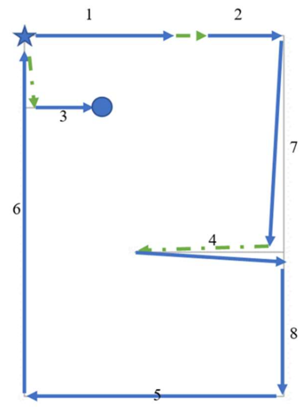
Consider the problem with nj joints and nw walls in which Wall i is defined by two vertices v
is and v
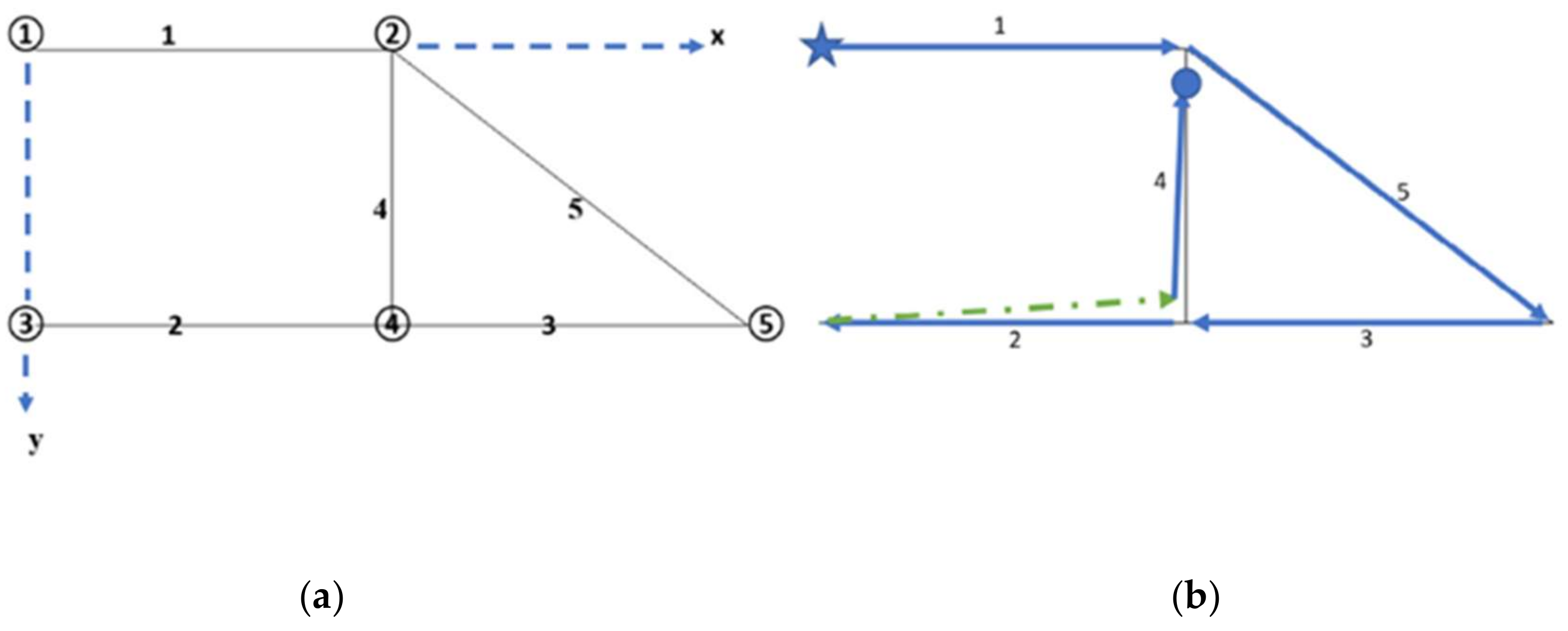
ie, that is, start and end joints, respectively. A simple example is presented in
Figure 1a, where nj and nw are both 5. The coordinates of the vertices are (0,0), (4,0), (0,3), (4,3), and (8,3), that is, from 1 to 5, respectively.
Table 1 explains the encoding scheme for this problem. To determine a path, random numbers between −1 and 1 are assigned to each nw-1 wall r
i, i = 2, 3, …, nw, as shown in Row a of
Table 1 for three candidate paths. It is assumed in all applications that the starting vertex is the first one, and concreting begins with Wall 1 from Joints 1 to 2. Therefore, the number assigned to the first wall is always zero.
Absolute values of these numbers, as shown in Row b, are then placed in order from lowest to highest, as shown in Row c. This becomes the order of operation for concreting the walls, as shown in Row d. Signs of the original random numbers indicate the direction in which the concreting will be executed. If the sign is positive, then the movement over the wall is positive (i.e., from starting vertex to end vertex). If the sign is negative, then the movement is in the opposite direction. In
Table 1, the order of execution of walls is shown in Row e.
The movements of the nozzle for the three candidates listed in
Table 1 are shown in
Figure 1b–d, respectively. In these figures, the starting point is marked with a star. The continuous lines in this figure indicate the concrete pouring actions, and the dashed lines denote the movements from one joint to another when no concrete is poured (i.e., idle movements that give the T value of the path).
Two types of nozzle movements are considered in this study. In the first approach, the nozzle moves parallel only to the x or y directions (i.e., in a rectangular manner); in the other, the nozzle can move from one joint to another following the shortest path (i.e., diagonally). In general, the results show that, as expected, the case involving rectangular movements is never better than the other case, although they are the same in some cases. It should also be noted that the value of T, which is to be minimized as previously explained, is the summation of the sections indicated by dashed lines in
Figure 1b–d. In these figures and in the following ones, the idle movements corresponding to rectangular movements are shown with green dashed ones, and with red dashed lines corresponding to diagonal movements.
For Candidates 1 and 2, the movements of the nozzle are the same regardless of whether diagonal movements are allowed. Thus, the figures drawn are valid for both cases. However, this is not the case for Candidate 3, where progressing to Wall 2 (i.e., after concreting Wall 1) is different for a nozzle depending on its capabilities, as can be seen in
Figure 1d. This affects the value of T also, which is 7 for rectangular movements and 5 when diagonal movements are allowed.
Among the paths considered relevant to the example in
Figure 1a, the best choices are the first and second for a nozzle moving in a rectangular manner or diagonally with T = 4. The worst choice is the third one, where T = 5 and T = 7 for nozzles moving in diagonal or rectangular directions, respectively.
Figure 1d shows that T = 5 is the direct distance from vertex 2 to vertex 3, and T = 7 is the distance between the same vertices via vertex 4.
3. Application of Harmony Search
HS is a population-based algorithm [
41]. To execute it, np number of vectors are first created, each representing a path as previously defined. These vectors form the original form of the harmony memory (HM). This is followed by finding T values of all paths and determining the best and worst among them. Normal cycles start after this introductory step. At each cycle, a new vector representing an additional path is created so that the number of vectors at hand becomes np + 1. The basic characterization of HS becomes decisive at this step. Parameters known as the HM considering rate (HMCR) and pitch adjusting rate (PAR), both with values between 0 and 1, are used. HMCR indicates that a new component of the new vector will be chosen with a probability of HMCR from those in HM; otherwise, it is arbitrarily in the feasible range. PAR indicates that the component chosen will not be taken as is but instead with a slight change with PAR probability. In the original study on HS [
41], these values were given as 0.95 and 0.10, respectively. After the np + 1
st vector is determined, its T value is calculated as with previous vectors. The last step in the cycle is to eliminate the vector with the worst T value such that np vectors in HM remain. These cycles continue until a decision is taken regarding the convergence of the procedure.
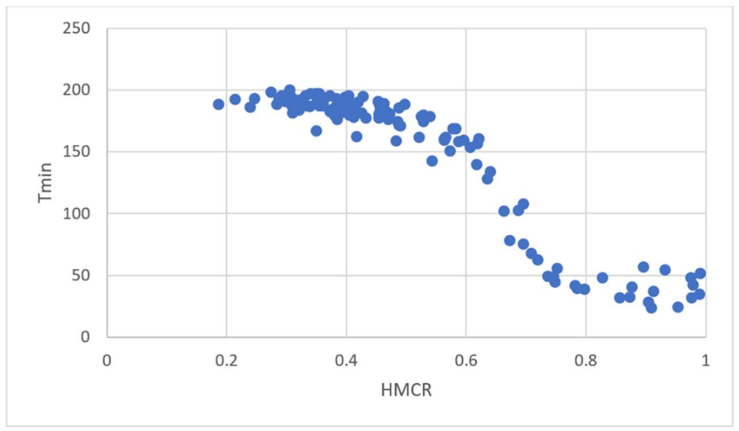
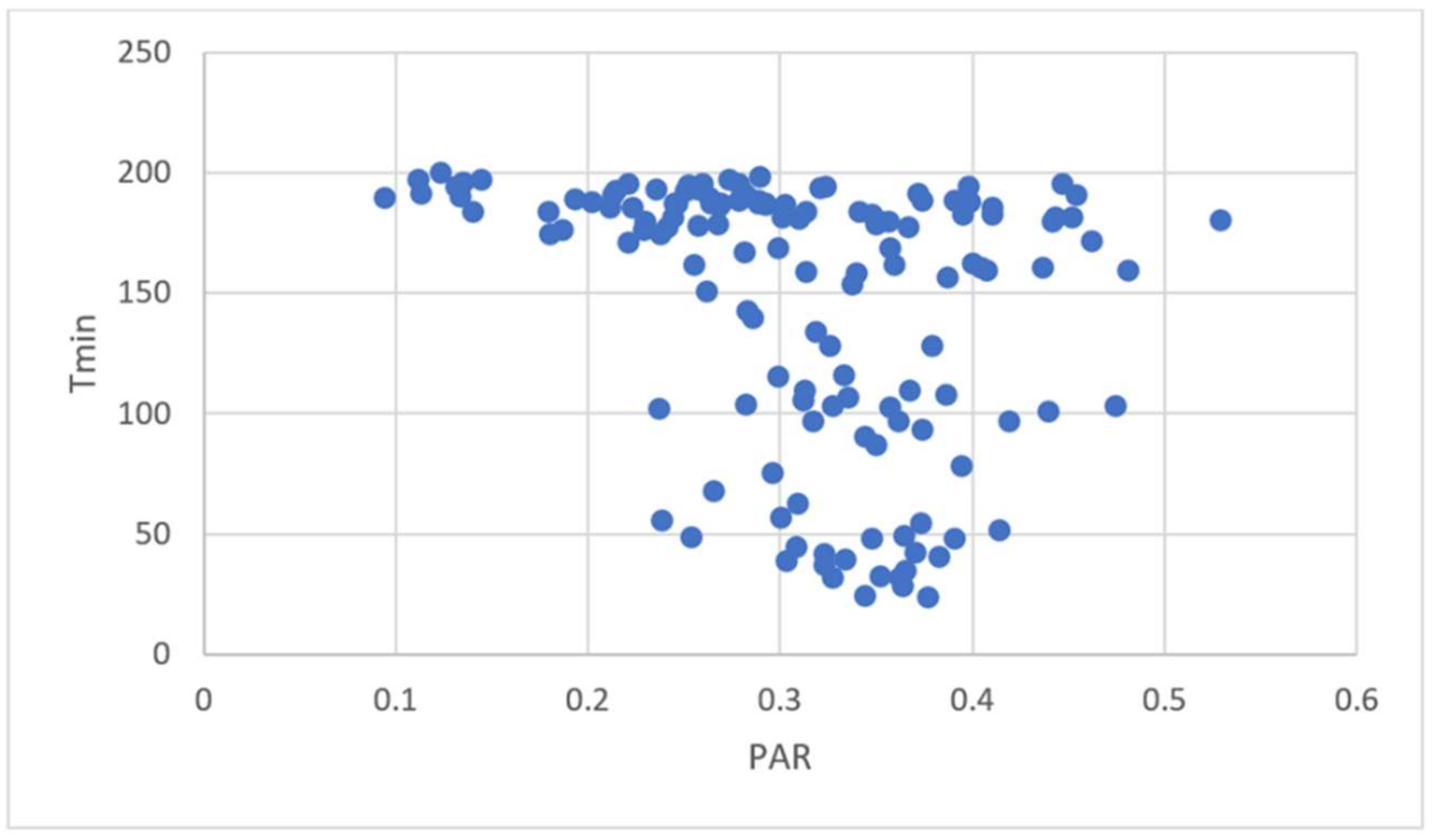
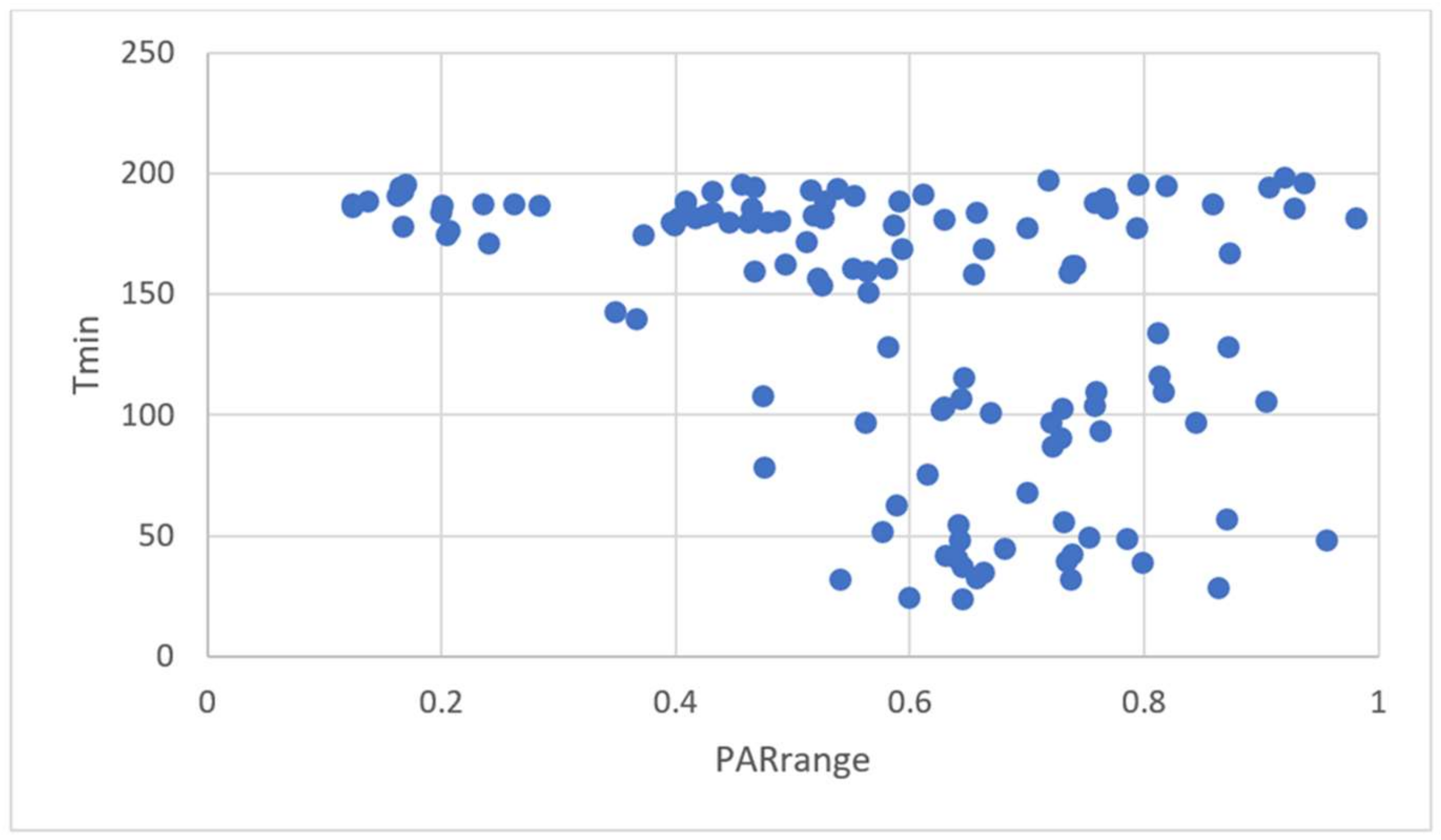
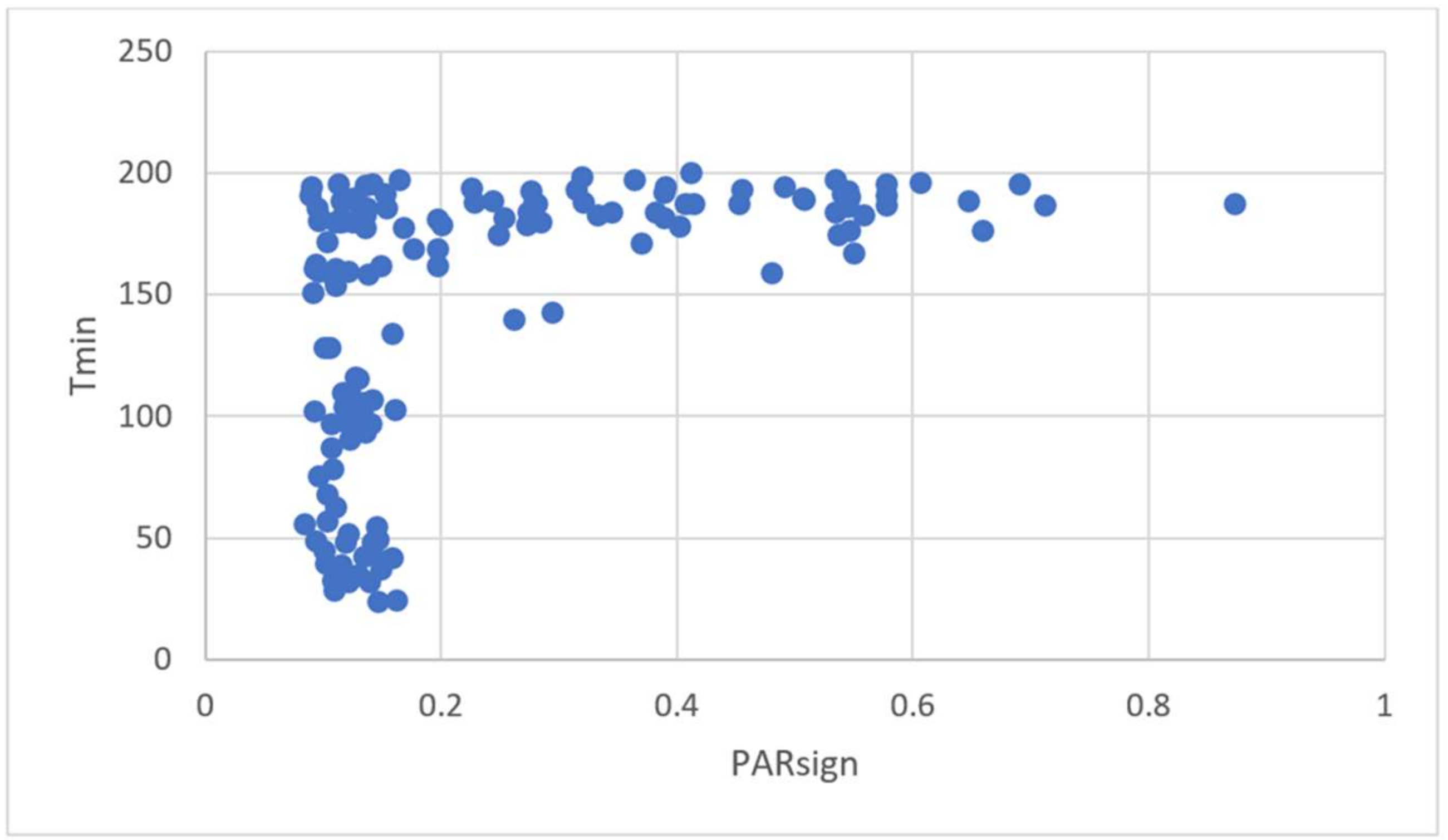
In the present study, a parameter search is conducted to find HMCR and PAR values that are particularly suitable for the current problem. This search is in fact enhanced to include two additional parameters. The first, called PARrange, is used to find the range in which slight changes would be made when pitch adjustment is applied. The second, called PARsign, is very specific to the problem considered, namely, the probability of changing the direction of pouring concrete into a wall from + (from start to end joint) to – (from end to start joint), or vice versa.
Parameter search is performed by making runs with different choices for all these four parameters, where the range searched becomes increasingly narrower. The results of these runs for HMCR are shown in
Figure 2.
Figure 3,
Figure 4 and
Figure 5 show the runs for PAR, PARrange, and PARsign, respectively. The parameters found are 0.95 for HMCR, 0.34 for PAR, 0.6 for PARrange, and 0.16 for PARsign, which can also be estimated from figures given. The value of 0.6 for PARrange initially seems to be somewhat high, but when one considers that in this analysis, the order of variables is important (i.e., as opposed to the number of correct digits in them), then this value is normal. Effectively, it is the order between the elements of the vector defining a path that is crucial. Therefore, to change the order, moving in large steps may be necessary. It should be noted that the search on parameters is performed with an important example (e.g., one with 31 walls) for this problem.
After the parameters of the algorithm are determined, HS is continued by eliminating the worst vector in HM until a certain number of cycles are completed. In all runs, the aforementioned parameters are used.
4. Numerical Examples
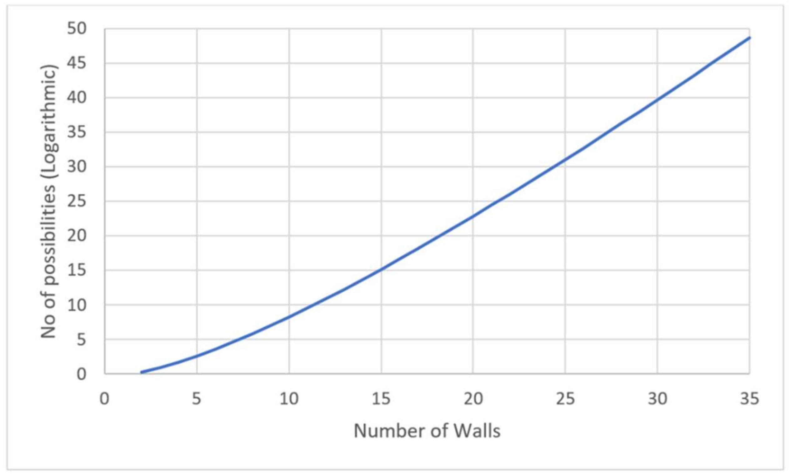
In this study, five examples were considered: flats with 7, 8, 14, and 31 walls, and a structural component with 17 walls. The first two examples (with seven and eight walls) were chosen because they are comparable to solutions found intuitively. The example of 14 walls can be considered as a medium-sized flat, whereas the fourth can be classified as a large flat for AMC applications. These four examples have openings corresponding to doors and corridors. The fifth example was chosen to be a structural component with no openings so that it can be manufactured in considerable numbers and used in assembling a larger structure.
In all these examples, to increase comparability, the starting point was chosen as Joint 1, and the first wall to be concreted was chosen as Wall 1, going from Joints 1 to 2. With this choice, the number of path possibilities is 2
nw−1(nw-1)!, where nw is the number of walls. This means that the possibilities for the seven-wall example is 46,080. This number is 645,120, 5.10118 × 10
+13, and 2.84813 × 10
+41 for the 8, 14, and 31-wall examples, respectively, and 1.3712 × 10
+18 for the structural component with 17 members (see
Figure 6). It is obvious that having so many path possibilities, it is not possible to choose the best path without recourse to a very elaborate method.
In the figures with examples, the number 1 vertex is marked with a star and is thus the starting joint. If the ending vertex is different than the starting one, it is marked with a large round point. The coordinate axes are like those shown in
Figure 1a (i.e., x is from left to right; y is from top to bottom).
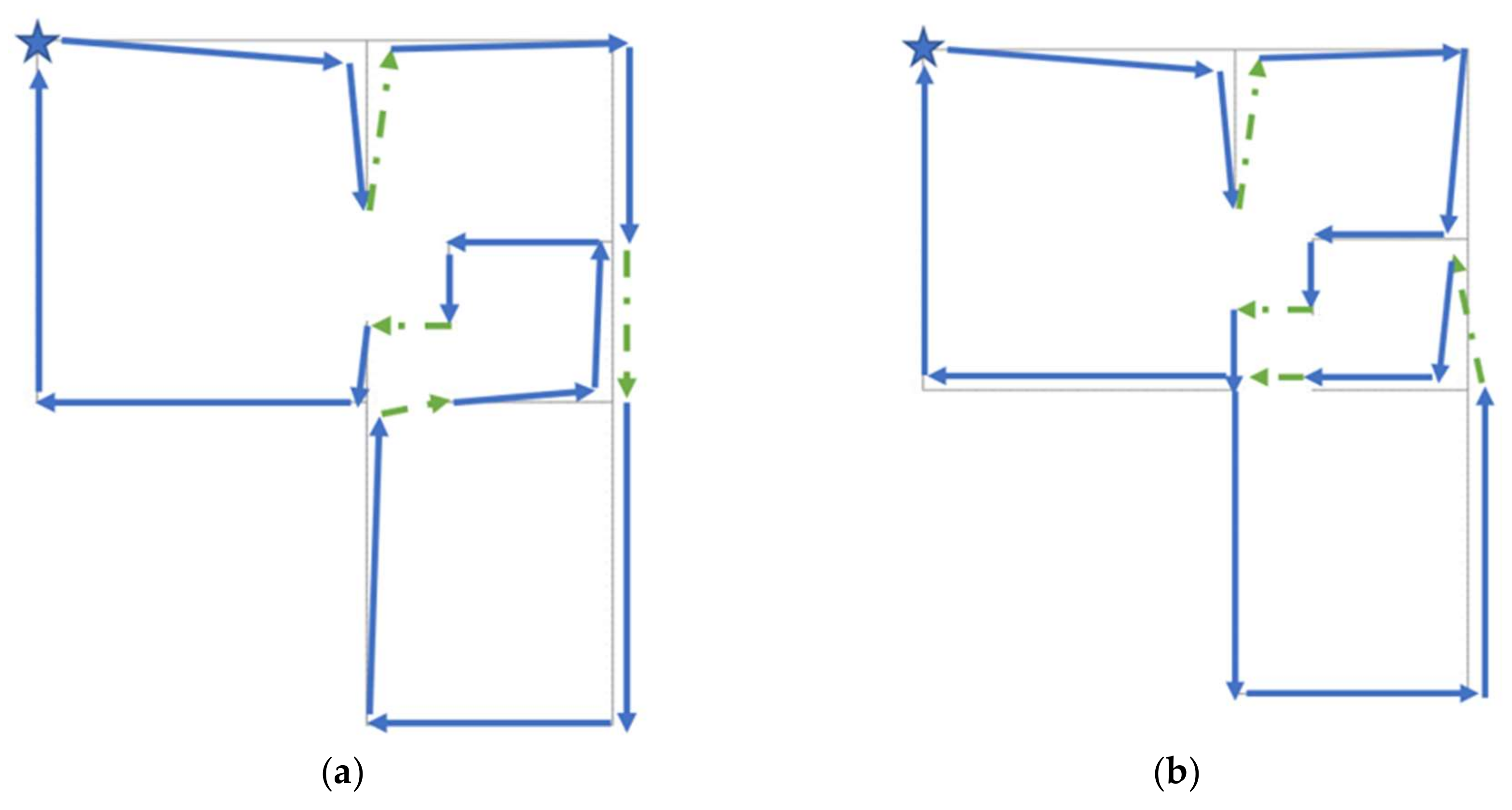
4.1. Example 1: Seven-Wall Floor
The first example has seven walls and eight joints. The shape of the corresponding flat is shown in
Figure 7.
Table 2 shows the joint coordinates and the start and end joints of walls. It is assumed that concrete is poured starting at Joint 1 on Wall 1 and progressing to Joint 2. The remaining part of the path is determined by the algorithm. As previously described, the movement of the nozzle between two joints when concrete is not poured is accomplished in two ways: one parallel to the coordinate axes x and y, the other by freely following the shortest distance between the two points, that is, by following the hypotenuse. The paths corresponding to these two cases are abbreviated in
Figure 7 and onwards with the letters R and D. Here R means that nozzle movements are only parallel to x and y axes, D means that diagonal movements are permitted too.
Six of the best solutions obtained for this problem are shown in
Table 3, where three solutions are for rectangular movements of the nozzle (marked with the letter R) and three are for diagonal movements of the nozzle (marked with the letter D). It can be seen that the best R and D solutions for this problem are the same (indicated by arrows in
Figure 7).
In the runs for this example, the population number is 20, and the maximum number of cycles for each run is 5000. Allure of a typical run is shown in
Figure 8. It can be seen that, for rectangular movements (i.e., for nozzle movements always parallel to the x and y axes), the shortest distance to travel is 25 units. The first solution shown in
Table 3 indicates that after Wall 1, a move will occur without concreting. The pouring of concrete will continue with Walls 2 and 6 and then proceed with Wall 3 in a negative direction after a movement without concrete being poured is made. This is followed by the concreting of Walls 7, 4, and 5, the last two being in negative directions. The T value (i.e., the objective function to be minimized for this path) is the sum of the distances traveled without concrete being poured.
In this problem, when diagonal movements are allowed, the best solution corresponds to that obtained for rectangular movements. In fact, the best solutions for both cases are exactly the same.
For this problem, although the theoretical possibilities can be calculated as 46,080, as previously given, determining the best solution by intuition is possible when examining the flat graph.
4.2. Example 2: Eight-Wall Flat
The second example is another in which the solution can be solved easily without employing computer methods, despite the fact that the number of possibilities is 645,120. This example has eight walls and 10 vertices, as shown in
Figure 9 and as listed in
Table 4.
As shown in
Table 5, the best solution obtained is again 35 units, where the nozzle is not obliged to move always parallel to the coordinate axes. It is also found in this case that, in the best solutions obtained, the nozzle moves parallel to the axes. The best solution in which the nozzle uses hypotenuses corresponds to a distance of 35.61553. This solution is not unique, where five other solutions are listed in
Table 6. The table shows that completely different paths may exist that give the same T value for a given problem.
It is found that 446 of 50,000 runs for the case of rectangular movements yield the same result, that is, T = 35, for the traveled distance. This corresponds to 0.89%, which means that nearly 1% of runs give a near optimal solution with no better solution to be found. For the case of non-rectangular movements, this percentage is somewhat less, that is, 0.78%, which corresponds to 391 best results in 50,000 runs.
It can also be observed that no specific trend in terms of best solutions exists that would enable surmising the next possible solution after considering those at hand. To emphasize this fact, the best solutions as shown in
Table 6 are chosen in such a manner that after Wall 1, any other wall can be poured in any direction, and so on.
It should also be noted that no one-to-one correspondence between solutions exists that corresponds to rectangular and non-rectangular (i.e., diagonal) nozzle movements. To show this,
Table 7 presents several solutions with an equivalent total duration (T = 35), which correspond to a 1, −8 start.
4.3. Example 3: 14-Wall Floor
The third example consists of a flat with 14 walls (see
Figure 10). The coordinates of the joints and wall connectivities are listed in
Table 8. The six best solutions are shown in
Table 9, three corresponding to the search with rectangular movements and three corresponding to the case in which diagonal movements are permitted. In all these solutions, T = 6, and the solutions given are all with rectangular movements despite the search in which diagonal movements are permitted.
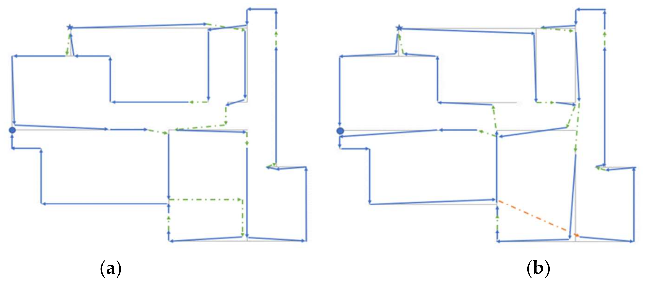
4.4. Example 4: 31-Wall Floor
Example 4 is a 31-wall flat (see
Figure 11). The coordinates of the joints and wall connectivities are listed in
Table 10. The six best solutions obtained are presented in
Table 11. The first three correspond to the search in which diagonal movements are not permitted (R) and the other three correspond to the other choice (D). The best solutions shown in
Figure 11 have a minimal idle distance of T = 19.5 for Case R and T = 18.27491 for Case D. Thus, as expected, the R solution is not better than the D solution in this case.
As previously explained, the number of path combinations for this problem is greater than 2.48 × 10
41. The results presented in
Table 11 were obtained after 45,000 runs for each Case R and D. Considering the huge number of path possibilities, the relatively modest number of runs showed that the algorithm presented can be considered as one with high performance.
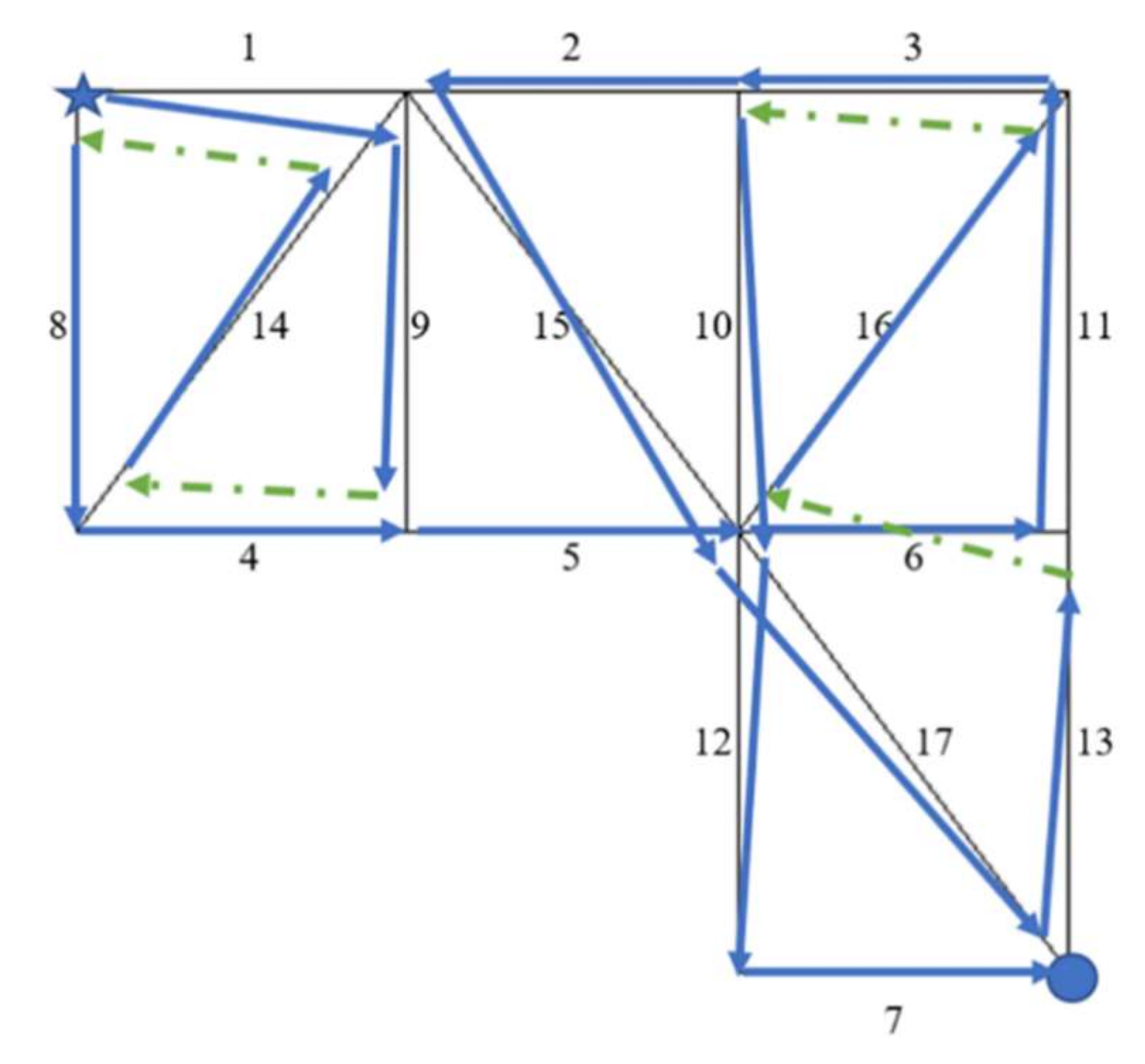
4.5. Example 5: 17-Member Structural Component
Example 5 is a structural component that will be manufactured in large numbers, and when assembled together with other components, will enable construction of a larger structure. This component is considered to have 17 members with no openings, as shown in
Figure 12. The geometry of the component is described in
Table 12. An analysis reveals that in the best solution for this problem, the number of idle movements is T = 12. Several solutions exist that yield a result of T = 12, where six of these solutions are presented in
Table 13. In
Figure 2, one solution is demonstrated that corresponds to the first result obtained in the search for an optimal path when diagonal idle movements are permitted.
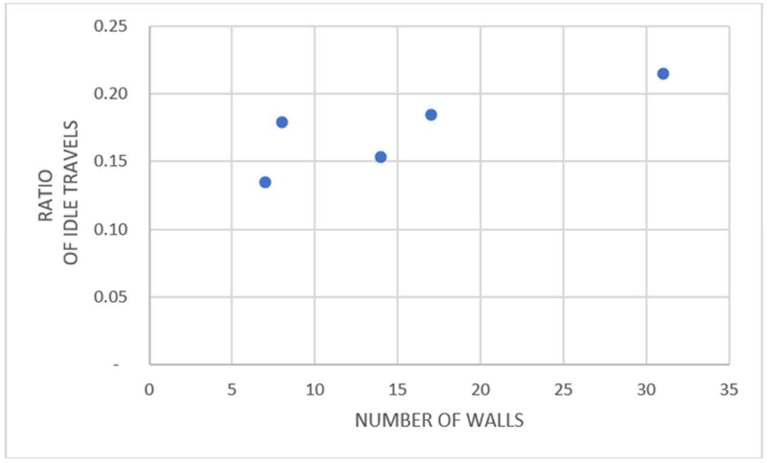
5. Discussion
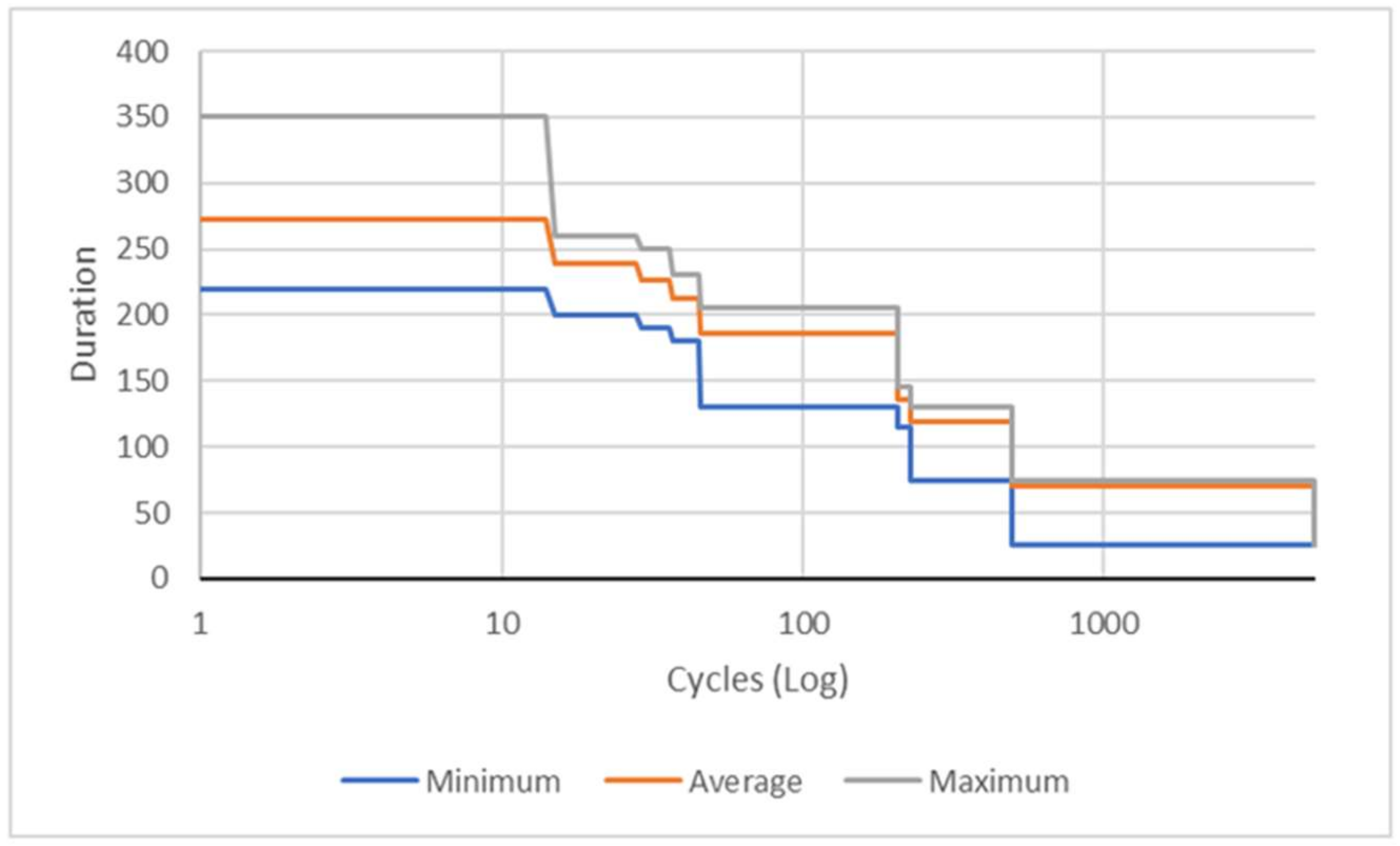
A general examination of the five problems solved showed that the ratio of idle movements of the nozzle to movements with concreting varied between 13% and 22%. This means that idle movements caused 12–18% of the total nozzle movements (see
Figure 13 and
Table 14). These percentages, which came out after an important optimization process, indicate that without a proper optimization, too much time and effort will be wasted in manufacturing structures and structural elements in construction industry.
6. Conclusions and Future Studies
In this study, a solution was presented for 2D path optimization problems that can be encountered, particularly in AMC applications and other similar areas. The structure in plane, which is in fact a single layer of a 3D form, consists of vertices and edges between them. The principal constraint of the problem is that some edges will be traveled at least once, and during that travel a manufacturing process will occur. In other edges, travel may occur or not, and the travels will be idle passages in which no manufacturing will be performed. It is assumed that the process will begin from a predefined vertex and progress through to a predetermined edge, and the rest of the path will be optimized by the algorithm defined.
Analyses on the problems solved in this study showed that distances covered by idle movements can be as much as 18% of the total distances traveled when a flat or structural component is concreted. This is a critical percentage and indicates that the optimization process considered in this study is essential to these operations. Clearly, if this type of optimization work is not conducted, more than 20% of the nozzle movements will be idle, which represents a major waste of time and energy.
Analyses showed that the number of possible paths in this type of problem increased rapidly as the number of edges increased, making the problem a nondeterministic polynomial (NP) one. For example, when the number of edges was 30, indicating that the problem being considered was common, the number of possible paths was 4.747 × 1039. It is also interesting to note that if the number of edges increased by 1 (i.e., from 30 to 31), the path possibilities increased to 2.801 × 1041, making the problem unsolvable by many algorithms. Metaheuristic algorithms represent a group of solutions that can be used for NP problems. In this study, the HS algorithm was chosen from among them. Computations showed that acceptable results were obtained with this choice. The study also revealed that 45,000 runs of HS were necessary to arrive at acceptable results for a problem with 31 walls. One research task for the future will be to identify a metaheuristic or hybrid algorithm to reduce this number.
In the 3D case, if the problem involves concrete pouring or a similar operation, constraints will exist that will make the problem much more difficult. Two of these types of constraints can be explained as follows.
- -
To pour concrete above a certain level, a specific setting time must pass so that the lower level acquires sufficient strength to carry the upper level.
- -
This waiting time cannot be too long, thus ensuring that the two levels are chemically connected to each other to work together.
The height of the levels and the setting time of the material will be new parameters with this problem. Computations will reveal that for some problems (i.e., in certain cases), no solution for a single nozzle will be available, and more nozzles used simultaneously will be necessary.
The optimization procedure discussed in this study may not be useful for cases in which a small number of structures are to be manufactured. However, if a considerable number is to be manufactured, the gain will be significant. Optimization will also be desirable when the manufacturing is performed under harsh conditions, as on the Moon or on Mars. Any percentage of time and energy gained under those conditions will be highly beneficial. Thus, one may conclude that research on path optimization with AMC and similar problems should continue until general solutions are obtained.
7. Data Availability
Some if not all data, models, or code that support the findings of this study are available from the corresponding author upon reasonable request. Data concerning the geometry of the models and some of the best solutions obtained are provided in this text. Run outputs and code developed are available upon reasonable request.


